Advances in Measurement Systems Part 11 pot
Bạn đang xem bản rút gọn của tài liệu. Xem và tải ngay bản đầy đủ của tài liệu tại đây (4.05 MB, 40 trang )
AdvancesinMeasurementSystems396
module has been added to control the different configurations of reconfigurable antenna
under test.
3.1 Signal processing
The signal processing subsystem deals with all the different modules which are related to
the OFDM signal, the software-radio and the channel estimation.
3.1.1 OFDM structure
Due to have a demonstrator of wideband, the OFDM technique will be used, since is very
efficient to transmit data over selective frequency fading channels. The main idea is to
divide in frequency a wideband channel in narrowband subchannels. Likewise, each
subchannel is a channel with flat fading despite of frequency-selective feature of a wideband
radio channel. To generate these subchannels in OFDM, an inverse of Fourier Fast
Transformation (IFF) is applied to one block of N data symbols:
1
0
2
)(
1
)(
N
k
N
knf
j
c
eKX
N
nx
(1)
In order to avoid inter-symbol interference due to the spreading of channel delay, a cyclic-
prefix block is inserted. This prefix is known as guard interval (GI), where the number of
samples of th prefix should be higher than the length of channel impulse response. The
effects of cyclic-prfix delete the ISI and convert the convolution between transmitted
symbols and channel in a circular convolution. Thus, the FFT is used at the receiver to
recover the block of data symbols. The synchronism module in the FPGA of the receiver is
based on (van de Beek et al., 1997). In Table 1 the most important parameters of the system
are detailed.
Parameter Symbol Value
Sampling frequency Fs 6.25 MHz
Useful symbol time Tu 1024/Fs=163.84 μs
Guard time Tg Ts/8=40.96 μs
Symbol time Ts 184.32 μs
Spacing between carriers Δf 1/Tu≈6.1 KHz
Number of carriers N 768
Bandwith BW 4687500 Hz
Table 1. Main testbed OFDM parameters
In the transmitter, a frame with 8 OFDM symbols is continuously generated, as shown in
Fig. 2. The first symbol is used for receiver synchronism and is a null symbol. After that, a
reference symbol which will be used to estimate the channel is introduced. And finally, 6
data symbols are included. These symbols are randomly generated since they are not going
to be evaluated, only the reference symbol to obtain the channel response.
WidebandMIMOMeasurementSystemsforAntennaandChannelEvaluation 397
Fig. 2. OFDM frame structure
3.1.2 Channel estimation
The channel estimation in MIMO systems is a very important stage, since in MIMO systems
the performances of algorithms depend on the accuracy of this estimation. The received
signal in each carrier is given by
kkkk
NXHR
(2)
where X is the vector of transmitted signals by each antenna, H indicates the MIMO channel
matrix and N represents the noise in the channel, all for each k-th subcarrier. The MIMO
channel matrix can be computed by
kMMkM
kMk
k
TRR
T
hh
hh
,,,1,
,,1,1,1
H
(3)
where each element of the matrix represents the channel response between each pair of
transmitter and receiver antennas.
On the other hand, different ways of obtaining the channel response have been studied. In
UMATRIX, orthogonal codes are used as pilots to let the receiver split the different
contributions from each antenna. Due to the maximum number of antennas is 4, a 4x4
matrix is needed. In our case, we use the following pilot matrix:
1111
1111
1111
1111
P
(4)
where the number of rows represents the space and the columns can represent either the
time or the frequency. In a firs option, the frequency axis was chosen, so in this way, the
AdvancesinMeasurementSystems398
channel is assumed invariant in 4 subcarriers. However, and with the aim of measuring
frequency selective channels, the time was as chosen axis in columns.
In order to get a better synchronization at the receiver, the pilot matrix P is multiplied by a
pseudorandom sygnal (S). Thus, at the receiver, for each k-subcarrier, we will have (2) with
PX
kk
S
(5)
And if it is chosen
1
H
kk
H
kk
XXXY
(6)
to estimate the channel, then the channel is multiplied by received signal Y, obtaining:
kkk
YRH
ˆ
kkkkk
S YNYPH
kkk
YNH
(7)
In Fig. 3. the estimated MIMO channel is plotted using the previous scheme of testbed. To
do it, each transmitter antenna was connected to each correspondent receiver antenna
(h
11
=h
22
=h
33
=h
44
=1), with the aim of testing the orthogonality of pilots.
Fig. 3. Orthogonality of the pilot code to estimate the channel
3.2 Antennas
For each combination of transmitter and receiver locations, three types of antennas have
been used: firstly the monopole array were utilized at both the receiver and the transmitter,
in order to evaluate the system performance when only vertical polarization is used.
WidebandMIMOMeasurementSystemsforAntennaandChannelEvaluation 399
Afterwards, the dual-polarized antennas (crossed dipoles) were used, so polarization
diversity is included in the system, to the cost of reducing spatial diversity (since the dual-
polarized dipoles are co-located). And finally, a planar inverted-F antenna (PIFA) array with
2 elements was placed to be evaluated (Gómez et al, 2008).
a) Monopoles
b) Cross-polarized dipoles
c) PIFAs
Fig. 4. Antennas under test
3.3 Measurements
3.3.1 UMATRIX application
One of the main objectives of the UMATRIX is that it has to allow measurements of
reconfigurable antennas in different environments. Thus, a tool with a friendly-user
interface and easy to use has been development in Matlab for the integration of processing
and measurement parts. In Fig. 5. the main window of the application is shown, where the
user goes checking the measured points, received signals and MIMO channel capacity
obtained.
AdvancesinMeasurementSystems400
Fig. 5. Main window of UMATRIX
Fig. 6.a) shows the transmitter of UMATRIX where the antenna array is located at the top.
All the transmitter is placed in a mobile platform to put it in several locations. On the other
hand, the receiver has a scanner which can sweep any point within an area of 6λx6λ (Mora et
al., 2008). Fig. 6.b) depicts the receiver with the scanner and the antenna array in the
scanner.
a)Transmitter b)Receiver
Fig. 6. Implementation of the testbed
3.3.2 Locations
All the measurements were taken in the ETSI de Telecomunicación (Madrid), in the fourth
floor of building C. In Fig. 7. different types of measurements can be distinguished
regarding the scenario: office and corridor. For the corridor environment, the transmitter
was put at the end of the corridor and the receiver was located in position 1 for LoS and
WidebandMIMOMeasurementSystemsforAntennaandChannelEvaluation 401
positions 2 and 3 for NLoS situations. In the case of office scenario, the transmitter was
placed in a laboratory (Tx B in Fig. 7.) and the receiver in another office.
Fig. 7. Map of locations in the measurements campaigns
3.3.2 Results
Once the channel is obtained in the receiver, the MIMO channel capacity is calculted.
Previously, the H matrix is normalized with the Frobenius norm. In order to remove the
path loss effect and study the diversity characteristics of the MIMO propagation channel,
the channel matrix H is usually normalized to obtain a fixed local signal to noise ratio for
each measured point. The use of this normalization is equivalent to considering a perfect
power control in the system. This is interesting to characterize the multipath richness and
diversity offered by the propagation environment, but it does not take into account the path
loss, shadow fading and penetration losses. Then the normalized channel will be
T R
M
i
M
j
ref
ij
ij
ref
RT
F
RTnorm
hh
MMMM
1 1
*
·
··
H
H
H
H
(8)
where I
MR
is the identity matrix of size M
R
xM
R
, M
T
is the number of transmitter antennas.
To compare the capacities for different types of antenna, a normalization with one antenna
array in each type of scenario has been done. On the other hand, as the channel state
information is not known at the transmitter, the capacity (in bps/Hz) in each k subcararier is
calculated from
H
kk
T
Mk
M
C
R
QHHI
Q
detlogmax
2
(9)
where Q is the covariance matrix of transmitted signals, such that Tr{Q} M
T
to account for
power constraint,
is the signal to noise ratio at the receiver, (·)
H
denotes Hermitian and
AdvancesinMeasurementSystems402
|A| is the determinant of matrix A. Two cases were considered in this analysis: no channel
state information (CSI) at transmitter and total CSI at transmitter. In the first case, the power
allocation strategy is assumed to be uniform, so that the channel capacity expression may be
simplified to
H
kk
T
Mk
M
C
R
HHI
detlog
2
(10)
When total CSI at transmitter is considered, the optimum waterfilling scheme is assumed to
allocate power, so the singular value decomposition (SVD) of H is realized, and the capacity
is computed as
K
i
iWF
C
1
ln
(11)
where (·)
+
denotes taking only those terms which are positive, and
i
is the i
(out of k) non-
zero eigenvalue of the correlation channel matrix R=HH
H
. The parameter
is chosen to
satisfy the power constraint
K
i
i
1
1
(12)
For 4x4 MIMO channel measurements, a comparison of single with dual-polarization
performances was realized for each scenario. Fig. 8. shows the capacity obtained for the
corridor scenario with LoS (position 1 of the receiver in Fig. 7.). As it is shown in Fig. 8.a),
the capacity increases with the spacing between elements, except for the case of 0.3λ. The
knowledge in the transmitter can give an extra capacity, as Fig. 8.b) depicts. The use of
Waterfilling scheme improve the performances in all the SNR range.
0.1 0.2 0.3 0.4 0.5 0.6 0.7 0.8 0.9 1
15.5
16
16.5
17
17.5
18
18.5
19
19.5
Capacity [bps/Hz]
d/
a) Capacity of monoples array as a function
of spacing with a SNR=20dB
0 5 10 15 20 25 30
5
10
15
20
25
30
SNR [dB]
Capacity [bps/Hz]
Monopoles d=
C
out,No CSI
C
out,WF
C
mean,No CSI
C
mean,WF
b) Comparison of monopoles capacity with
a spacing of λ, as a function of SNR and CSI
Fig. 8. Capacity of monopole array.
On the other hand, the importance of using single or dual polarization has been also
studied. Fig. 9. represents the CDF of the capacity for all the monopole array spacings and
WidebandMIMOMeasurementSystemsforAntennaandChannelEvaluation 403
the cross-polarized dipole array. It is shown that for LoS the employ of dual polarization
enhances the performances with respect to the MIMO channel capacity. However, for NLoS
cases, the use of dual polarization does not have a great impact on the performances.
5 10 15 20 25 30
0
0.1
0.2
0.3
0.4
0.5
0.6
0.7
0.8
0.9
1
Capacity [bps/Hz]
P(C<abcissa)
M d=0.1
M d=0.2
M d=0.3
M d=0.4
M d=0.5
M d=0.6
M d=0.7
M d=0.8
M d=0.9
M d=
Dipoles
a) CDF capacity of corridor LoS (position 1
of Fig. 7.)
10 12 14 16 18 20 22 24 26 28 30
0
0.1
0.2
0.3
0.4
0.5
0.6
0.7
0.8
0.9
1
Capacity [bps/Hz]
P(C<abcissa)
M d=0.1
M d=0.2
M d=0.3
M d=0.4
M d=0.5
M d=0.6
M d=0.7
M d=0.8
M d=0.9
M d=
Dipoles
b) CDF capacity in NLoS scenario (position
3 of Fig. 7.)
Fig. 9. Comparison of the CDF capacity for single and dual polarization antennas.
Moreover, 4x2 MIMO channel measurements were carried out to compare the MIMO
channel capacity by using different radiating elements. Fig.10. compares the CDF of the
capacity obtained for monopoles, dipoles and PIFAs in different scenarios, with LoS and
NLoS. It can be concluded that for two radiating elements at the receiver side, MIMO
channel capacity strongly depends on the antenna characteristics, such as radiation pattern,
mutual coupling and spacing between elements.
4 6 8 10 12 14 16 18 20
0
0.1
0.2
0.3
0.4
0.5
0.6
0.7
0.8
0.9
1
Capacity [bps/Hz]
P(C<abcissa)
Monopoles-Monopoles
Monopoles-PIFAs
Dipoles-Dipoles
Dipoles-PIFAs
a) CDF capacity of corridor LoS (position 1 of
Fig. 7.)
4 6 8 10 12 14 16 18 20
0
0.1
0.2
0.3
0.4
0.5
0.6
0.7
0.8
0.9
1
Capacity [bps/Hz]
P(C<abcissa)
Monopoles-Monopoles
Monopoles-PIFAs
Dipoles-Dipoles
Dipoles-PIFAs
b) CDF capacity in NLoS scenario(position
4 of Fig. 7.)
Fig. 10. Comparison of the CDF capacity for 4x2 MIMO channels with different antennas
AdvancesinMeasurementSystems404
4. MIMO prototype for DVB-T2 system
DVB-T2, the second generation of the DVB proposal for digital terrestrial TV, has been
recently proposed by DVB project (dvb) as an evolution of DVB-T when the shutdown of
analog television process will be finished. In order to give a newer technical response to the
necessity the digital dividend, process by which some free frequencies at UHF used by
analog TV will be assigned to different services (3G/4G), DVB-T2 will improve frequency
efficiency to provide multicast in HD with the same 8 MHz channel.
As DVB-T, DVB-T2 expects to be received in plugged TV terminals in mobile environment
or with unplugged terminals in indoor or in low speed (pedestrian) environments, so a
MISO scheme has been included, transmitting with a distributed Alamouti block code.
However, in order to go further a full MIMO scheme is proposed in this paper, which may
be similar to the one that will be included in NGH (second generation of DVB-H) in the next
future, obtaining a very efficient performance in highly Doppler environments, that is to
terminals (unplugged or not) operating in high speed vehicles.
On the other hand, DVB-T2 will provide higher efficiencies in frequency than the nowadays
DVB standard DVB-T. DVB-T2 proposal considers the inclusion of MISO technology but not
MIMO. MIMO will be considered in future revisions and it will provide a further increment
of frequency efficiency mainly in harsh scenarios as strong multipath environments or
highly Doppler radio channels.
In order to evaluate the performances of a DVB-T2 system in realistic scenarios, the use of a
real platform is of great interest, since it enables to include several aspects that are not
usually addressed in theoretical studies or simulations, such as the effect of different
antennas or scenarios (Gómez-Calero et al., 2006). In this section, a novel 2x2 MIMO testbed
for DVB-T2 has been designed and implemented in order to test the enhancement obtaining
by the using of multiple antennas at each side of the radio link for UHF band, particularly at
frequency of 594 MHz.
The general architecture of the testbed is depicted in Fig. 11., where 2 antennas can be
placed at the transmitter and the receiver side. The DVB-T2 signals are generated off-line in
a PC (e.g. using Matlab) and then they are sent to the Software-Defined-Radio (SDR)
platform. This platform receives the signals and transmits them in real-time and in
Intermediate Frequency (IF) to the RF module. Finally, signals are upconverted to RF
frequency, amplified and filtered, and then transmitted to the radio channel by the antenna
array. In the receiver, the signals are captured by the antenna array and downconverted,
amplified and filtered by the RF module. Finally, the SDR realizes the synchronization and
FFT previous to send the signals to the PC.
WidebandMIMOMeasurementSystemsforAntennaandChannelEvaluation 405
Fig. 11. General architecture of the MIMO measurement system for DVB-T2
4.1 Signal processing
The most complex part of the testbed is the signal processing module, since it supports all
the digital to analog and analog to digital conversions (DAC and ADC) and the processing
of the OFDM signal with the synchronization and the use of the Fast Fourier Transmorm
(FFT). In the following subsections the transmitted DVB-T2 signals and SDR platform are
explained.
4.1.2 DVB-T2 structure
The DVB-T2 frame structure is divided in three different parts (ETSI, 2008). The first one is
the P1 symbol which is used to do a faster detection and frequency synchronization. Then,
the P2 symbol is transmitted to indicate the type of encoders and data configuration of the
data symbols. However, for the sake of simplicity in this testbed the P2 symbol is removed.
Finally the data symbols are sent with the user data and pilots for the channel estimation.
The block diagram of the transmitter is shown in Fig. 12. Data are generated and passed to
the MIMO encoder which applies the distributed Alamouti to transmitt the signals by each
antenna and then to recover the data symbols in the receiver. The Alamouti scheme
(Alamouti, 1998) is modified with the scheme detailed in Table 2.
Fig. 12. Block diagram of the transmitter signal processing
Subcarrier Tx antenna 1 Tx antenna 2
k
i
s
1
-s
2
*
k
i+1
s
2
s
1
*
Table 2. Alamouti modified scheme
After that, the continual and scattered pilots are inserted to estimate the channel at the
receiver. Then, the Inverse-FFT (IFFT) is done and the Guard Interval (GI) is inserted in
order to avoid inter-symbol interference (ISI) due to the channel delay spread. The cyclic-
prefix removes the ISI and converts the convolution between transmitted symbols and
channel into a circular convolution. Finally, the P1 symbol is inserted and the two signals
are converted from digital to analog and sent to RF module.
AdvancesinMeasurementSystems406
4.1.3 Sowtfare-Radio
For the real-time process, two XtremeDSP boards based on the BenADDA module of
Nallatech have been used: one for the transmitter and one for the receiver. Each board has a
FPGA VirteX II Pro V2P30 and 4 MBytes of SRAM memory with 2 DACs of 160 MHz and 2
ADCs of 105 MHz (Nallatech).
Fig. 13. shows the architecture of the transmitter. The data symbols are sent to the board via
DMA through the PCI bus. The DMA SRAM IFACE module stores them in the board
external memory ZBT SRAM. The maximum capacity is 512 samples per channel. Once the
data write cycle is finished, the same module reads them from the memory and extracts
them in a continuous and cyclic way. The I/Q data streams of each channel go to Digital Up
Converter module, where the signals are interpolated by a factor of 10 and are upconverted
to an IF of 36 MHz. The data are sent to DACs, which operate at a frequency of 91428571 Hz.
This frequency is selected for being 10 times the inverse of the sample period of a 8 MHz
channel, which according to the DVB-T2 standard (ETSI, 2008) is T=7/64 μs.
Fig. 13. Architecture of SDR transmitter
Fig. 14. Architecture of SDR receiver
WidebandMIMOMeasurementSystemsforAntennaandChannelEvaluation 407
On the other hand, Fig. 14. represents the main blocks of receiver subsystem. The signal
from channel 1 is used to obtain the synchronism in time domain of received symbols. The
synchronism algorithm is based on the correlation of the cyclic prefix of OFDM symbols
(van de Beek et al., 1997). Then, the signals go to Time Synch module which generates the
synchronism signal which allows to obtain the OFDM symbols in the next module, named
Guard Interval Removal. Finally, the FFT is done to recover the block of data symbols.
In order to estimate the beginning of the frame, the signal passes through a correlator with
the P1 symbol. Fig. 15. represents the correlation of a frame made up a P1 symbol and 9 data
symbols.
0 1 2 3 4 5 6
x 10
4
0
200
400
600
800
1000
1200
Samples
Corr. Data
Corr. P1
Fig. 15. Correlation of received signals. Red line represents the correlation with the P1
symbol and blue line shows the autocorrelation with the data symbol
4.1.5 Channel estimation
One of the key aspects in MIMO is the channel estimation, since MIMO system
performances depend on the accuracy of the estimated channel matrix. Due to the selection
of 2K mode of FFT and a GI of 1/8, the DVB-T2 standard (ETSI, 2008) proposes the PP1
pattern for scattering pilots for MISO.
The scattered pilots, for each OFDM symbol are placed each 12 subcarriers along the
frequency axis. Attending to the temporal axis, the pilots start in the first subcarrier and the
initial point is shifted in 2 subcarriers for the following 3 OFDM symbols, as Fig. 16.a) and
Fig. 16.b) show for antenna 1 and 2, respectively. Thus, the pilots structure is done in 4-
symbol blocks in time domain and it depends on the used antenna. In antenna 2 case (Fig.
16.b), the corresponding pilots to symbols 1 and 3 are inverted to distinguish the transmitter
antenna. Moreover, it is worth mention here that the scattering pilots are generated
according to a pseudorandom sequence and PRBS (ETSI, 2008).
AdvancesinMeasurementSystems408
a) Antenna 1
b) Antenna 2
Fig. 16. Scattered pilots distribution
Thus, if X
k
represents the transmitted symbols vector for both antennas for the k-subcarrier,
the received vector R
k
is given by (2). Due to the testbed has two antennas in the transmitter
and other two in the receiver, the MIMO channel matrix is represented by
kk
kk
k
hh
hh
,2,2,1,2
,2,1,1,1
H
(13)
where each matrix element indicates the subchannel between each pair of transmitter-
receiver antenna.
In the literature a MIMO channel estimator for DVB-T2 has not been proposed, so in this
section an original scheme is presented to estimate the channel for MIMO case. First of all,
the channel is asummed not to vary in time domain for 4 data symbols, similar to other
channel estimators for DVB-T (Lee et al., 2007, Palin & Rinne 1999, Chen et al., 2003, Fang &
Ma, 2007). Therefore, the pilots are gathered in groups of 4 OFDM data symbols in only one
symbol, obtaining one pilot subcarrier out of 3 subcarriers. Fig. 17. depicts the association
for both antennas.
Fig. 17. Scattered pilots association for antennas 1 and 2
WidebandMIMOMeasurementSystemsforAntennaandChannelEvaluation 409
The received signals in antennas 1 and 2, r
1,k
and r
2,k
, respectively, for the k-subcarrier are
given by
r
1,k
=x
1,k
· h
11,k
+ x
2,k
· h
12,k
+ n
1,k
r
2,k
=x
1,k
· h
21,k
+ x
2,k
· h
22,k
+ n
2,k
(14)
where x
i,k
represents the pilot signal transmitted by antenna i, and n
i,k
is the noise
contribution in antenna i. From this point Here, two cases are considered to estimate the
channel. The first one is the case in which the pilots of both antennas are scattered pilots for
a given subcarrier. This case is marked with A in Fig. 17. In the other case, the pilot for one
antenna is a scattered pilot and for the other antenna is an inverted scattered pilot, for a
given subcarrier. This is case B in Fig. 17.
Thus, for case A the received signals are
r
a
1,k
= x
a
1,k
· h
11,k
- x
a
1,k
· h
12,k
+ n
a
1,k
= x
a
1,k
· (h
11,k
- h
12,k
)+ n
a
1,k
(15)
r
a
2,k
= x
a
1,k
· h
21,k
- x
a
1,k
· h
22,k
+ n
a
2,k
= x
a
1,
k
· (h
21,k
– h
22,k
)+ n
a
2,k
(16)
And for case B
r
b
1,k
= x
b
1,k
· h
11,k
+ x
b
1,k
· h
12,k
+ n
b
1,k
= x
b
1,k
· (h
11,k
+ h
12,k
)+ n
b
1,k
(17)
r
b
2,k
= x
b
1,k
· h
21,k
+ x
b
1,k
· h
22,k
+ n
b
2,k
= x
b
1,
k
· (h
21,k
+ h
22,k
)+ n
b
2,k
(18)
Operating with the obtained signals from (15)-(18), channel coefficients can be estimated as
a
k
b
k
a
k
b
k
a
k
k
x
x
x
rr
h
,
,
,
,,
,,
~
1
1
1
11
11
2
(19)
a
k
b
k
a
k
b
k
a
k
k
x
x
x
rr
h
,
,
,
,,
,,
~
1
1
1
11
21
2
(20)
a
k
b
k
a
k
b
k
a
k
k
x
x
x
rr
h
,
,
,
,,
,,
~
1
1
1
22
12
2
(21)
a
k
b
k
a
k
b
k
a
k
k
x
x
x
rr
h
,
,
,
,,
,,
~
1
1
1
22
22
2
(22)
AdvancesinMeasurementSystems410
And the estimated MIMO channel matrix is
kk
kk
k
hh
hh
,,,,
,,,,
~~
~~
~
2212
2111
H
(23)
4.2 RF-FI
In the transmitter, the RF stage receives the signal from signal proccesing module and
upconverts from IF (36 MHz) to RF frequency (594 MHz). Then, the signal is filtered and
amplified, with a transmitted power of +2 W rms. In order to upconvert the signals of both
branches 1 and 2, a direct digital synthesizer (DDS) is used.
In the receiver, the signals are received from antenna ports and then are amplified, filtered
and downconverted to IF. In this case, a voltage controlled attenuator is placed to adapt the
recevied signal power to the best range of levels. The variation of the attenuator is from 3 dB
to 38 dB in steps of 5 dB.
4.3 Antenna array
The MIMO testbed has two antennas at the transmitter and two at the receiver, respectively.
The antennas have been designed for the testbed to work at 594 MHz. The radiating element
is a dipole with a reflector element. The reflection coefficient of the transmitter and receiver
antennas is depicted in Fig. 18.a). It shows that all the implemented antennas have a good
matching at desired frequency band, obtaining a reflection coefficient lower than -17 dB. On
the other hand, the radiation pattern is presented in Fig. 18.b), where the XPD is higher than
25 dB in the maximum direction of θ=0º.
500 550 600 650 700
-20
-18
-16
-14
-12
-10
-8
-6
-4
-2
0
Frequency [MHz]
|S
11
| [dB]
Tx 1
Tx 2
Rx 1
Rx 2
a) Reflection coefficient of the
antennas
b) Measured radiation pattern of an
antenna
Fig. 18. Antenna performances
WidebandMIMOMeasurementSystemsforAntennaandChannelEvaluation 411
4.5 Measurements in indoor/outdoor scenarios for different polarizations
Once the different modules of transmitter and receiver are implemented and work properly,
the integration of all of them is done. In Fig. 19. the transmitter and receiver are illustrated.
The transmitter is placed on a 19" rack and the received is mounted on a mobile platform in
order to measure different environments.
a) Transmitter
b) Receiver
Fig. 19. Integration of the testbed
As in any real system, implementation issues such as frequency errors by using different
local oscillators internal clocks at each side of the radio link appear. In general, all the errors
can be represented as
kkkkk
fTsk
Tu
t
k
Tu
Td
kj NIXHR
222
0
exp
(24)
where T
d
represents the symbol temporal offset, Δ
t
the sampling temporal offset, φ
0
the
phase offset, Δ
f
the frequency offset and I
k
is the ICI (Inter-Carrier Interference) due to
frequency offset for the k-carrier. These errors must be taken into account and have been
mitigated in the signal processing module.
Once the MIMO testbed has been realized, a measurement campaign has been carried out in
order to evaluate the enhancement obtained by using the MIMO scheme. The measurements
were carried out in the E.T.S.I of Telecommunications School, at Universidad Politécnica de
Madrid, Spain. The transmitter was situated on the rooftop of building C with a spacing
between elements of λ. Fig. 20. depicts the topview of the measurement locations. In order to
measure several scenarios, the receiver was located in three different positions. In position 1,
the receiver was placed in the parking area of the building in LoS (Line of Sight). The
AdvancesinMeasurementSystems412
receiver for NLoS (Non Line of Sight) was situated in position 2, in the parking of the next
building. Finally, for the indoor scenario, the receiver was located in the third floor of the
building, as Fig. 20. shows. For each scenario, three different polarization schemes were
evaluated: HH, HV and VV, where H and V means horizontal and vertical polarization for
antennas 1 and 2 both in the transmitter and the receiver, respectively.
Fig. 20. Top view of the Tx and Rx positions
4.5.1 MIMO channel
The first step for evaluating the MIMO channel is to normalize channel power. After chanel
estimation, the channel power is calculated for all the measured cases. The channel power is
averaged over all frequencies f
v
and temporal snapshots t
u
and is calculated by
RT
N
i
N
j
vu
avr
MM
ftP
P
t
f
1 1
,
(25)
where N
t
represents the number of OFDM symbols (100 in this case), N
f
indicates the
number of subcarriers (2048) and P represents the mean power in the measured point and is
given by
RT
Fvu
vu
MM
ftP
ftP
2
||,||
,
(26)
Table 3 shows the comparison of mean power for each scenarios as a function of antenna
polarization. It is shown in LoS scenarios, the received power is increased. However, in
indoor case the power only is reduced in 6 dB because the distance between the transmitter
and receiver is about 23 m smaller than in the case 3.
WidebandMIMOMeasurementSystemsforAntennaandChannelEvaluation 413
Measured
scenario
Mean channel power (dB)
HH HV VV
1 - Outdoor LoS -63.5 -62.8 -63.2
2 - Outdoor NLoS -81.1 -81.8 -73.7
3 - Indoor NLoS -67.9 -68.8 -69.5
Table 3. Comparison of measured mean power
4.5.2 MIMO capacity
Besides the diversity gain, the other important of MIMO channels is the increase of the
channel capacity. In the case of DVB-T2, the transmitter does not know the Channel State
Information (CSI), and the MIMO capacity can be calculated from
N
k
H
kk
T
Mk
M
C
R
1
2
HHI
detlog
bps/Hz
(27)
where M
R
and M
T
represent the number of receiver and transmitter antennas, respectively, k
is the given subcarrier, N represents the total number of subcarriers and ρ is the Signal to
Noise Ratio (SNR). The measurements have been realized with M
T
=M
R
=2.
With the aim of comparing the capacity of SISO and MIMO, Fig. 21. represents the
cummulative distribution function of the capacity calculated for the LoS case with
polarization diversity. The capacity increases in the 2x2 case.
2 4 6 8 10 12 14 16
0
0.1
0.2
0.3
0.4
0.5
0.6
0.7
0.8
0.9
1
CDF
Capacity [bps/Hz]
SISO
MIMO
Fig. 21. Comparison of CDF of capacity with 1x1 and 2x2 in outdoor LoS case with
polarization diversity
On the other hand, Fig. 22. shows the comparison of all the cases comparing the use of
different polarization schemes. The highest values of capacity are obtained for indoor NLoS,
followed by outdoor NLoS and the, outdoor LoS, except when polarization diversity (HV) is
used in LoS case, since the obtained outage capacity at 10% is the highest.
Attending to outage capacity, the highest values are obtained for the outdoor LoS HV case
and the indoor situations for all the polarization schemes.
AdvancesinMeasurementSystems414
Fig. 22. CDF of capacity for all the measured scenarios
5. Conclusions
In the last decade, Multiple-Input Multiple-Output (MIMO) systems have created a great
interest in research. Many works shows an increase in terms of data bit rate by using several
antennas at each side of the radio link. In this chapter, two novel measurement systems for
MIMO channels in indoor environment are presented. In order to study the propagation
characteristics of these systems, using both polarization and spatial diversity in multi-
antenna systems can be evaluated, thanks to the use of different types of antennas.
On one hand, a novel MIMO-OFDM testbed (UMATRIX), designed and implemented in the
UPM, has been used to accomplish the measurements at 2.45 GHz. The UMATRIX has
several characteristics which makes it good for antenna reconfigurable measurements.
OFDM technique is introduced to measure the wideband MIMO channel response, so a
FPGA-based receiver has been developed. A measurement campaign to compare the system
performance with either single-polarized or dual-polarized antennas was conducted in an
indoor scenario, including multiple locations for the transmitter module. From the capacity
analysis, it may be concluded that in indoor environment for corridor scenario, dipoles
present better performances than monopoles. However, in NLoS office scenario, monopoles
outperforms the dual-polarized antennas. Finally, higher capacity is obtained with higher
spacing between radiating elements, due to less correlation among the MIMO subchannels.
On the other hand, a new 2x2 MIMO testbed has been designed and implemented for the
future digital television system DVB-T2. The testbed is based on software radio platforms
where the signal processing is implemented according to the standard. The testbed has been
designed to carry out measurements at the frequency of 594 MHz. A measurements
campaign has been done in outdoor and indoor scenarios. Results show the importance of
using multiple antennas at each side of the radio link for increasing the capacity of the
MIMO system. Moreover, it has also been shown that polarization diversity provides an
additional capacity gain especially for outdoor LoS cases (up to 4 bps/Hz in outage
capacity).
WidebandMIMOMeasurementSystemsforAntennaandChannelEvaluation 415
6. References
Adjoudani, A.; Beck, E.; Burg, A.; Djuknic, G. M.; Gvoth, T.; Haessig, D.; Manji, S.; Milbrodt,
M.; Rupp, M.; Samardzija, D.; Siegel, A.; Sizer II, T.; Tran, C.; Walker, S.; Wilkus,
S.A.; Wolniansky, P., “Prototype Experience for MIMO BLAST over Thrid
Generation Wireless System,” Special Ussue JSAC on MIMO Systems, vol 21, pp.
440-451, April 2003.
Alamouti, S., “A simple transmit diversity technique for wireless communications,” IEEE
Journal on Selected Areas in Communications, vol. 16, pp. 1451–1458, October 1998.
Aschbacher, E.; Caban, S.; Mehlfuhrer, C.; Maier, G.; Rupp, M., “Design of a flexible and
scalable 4x4 MIMO testbed,” IEEE 11
th
Digital Signal Processing Workshop, 2004
and the 3
rd
IEEE Signal Processing Education Workshop. 1-4 Aug. 2004, pp. 178-
181.
Batariere, M. D.; Kepler, J. F.; Krauss, T. P.; Mukthavaram, S.; Porter, L. W.; Vook, F. W., “An
experimental OFDM system for broadband mobile communications,” IEEE
Vehicular Technology Conference, v 4, n 54ND, 2001, p 1947-1951.
Chen, S H.; He, W H. ; Chen, H S. & Lee, Y., “Mode detection, synchronization, and
channel estimation for DVB-T OFDM receiver,” in IEEE Global
Telecommunications Conference, 2003. GLOBECOM ’03, vol. 5, Dec. 2003, pp.
2416–2420 vol.5.
Dvb .
Ellingson S. W., “A flexible 4x16 MIMO testbed with 250 MHz – 6 GHz tuning range,” IEEE
Antennas and Propagation Symposium, Washington, DC, July 2005.
ETSI, “Digital Video Broadcasting (DVB);Frame structure channel coding and modulation
for a second generation digital terrestrial television broadcasting system (DVB-
T2),” Draft ETSI EN 302 755 V1.1.1 (2008-04), 2008.
Fang, R D. & Ma, H P., “A DVB-T/H Baseband Receiver for Mobile Environments,” in
2007 WSEAS International Conference on Circuits, Systems, Signal and
Telecommunications, Queensland, Australia, January 2007.
Foschini, G. & Gans, M., “On Limits of Wireless Communications in a Fading Enviroment
when Using Multiple Antennas,” Wireless Personal Communications, vol. 6, pp.
311–335, March 1998.
GmbH, “RUSK MIMO: Broadband Vector Channel Sounder for MIMO Channels,” MEDAV
2001. Available at
Goldsmith, A.; Jafar, S.; Jindal, N & Vishwanath, S., “Capacity limits of MIMO channels,”
IEEE Journal on selected areas in communications, vol. 21, no. 5, June 2003.
Gómez-Calero, C.; García-García, L.; Martínez, R. & de Haro, L., “Comparison of antenna
configurations in different scenarios using a wideband MIMO testbed,” IEEE
Antennas and Propagation Society International Symposium 2006, pp. 301–304,
July 2006.
Gómez-Calero, C.; González, L. & Martínez, “Tri-Band Compact Antenna Array for MIMO
User Mobile Terminals at GSM 1800 and WLAN bands,” Microwave and Optical
Technology Letters, vol. 50, no. 7, pp. 1914–1918, July 2008.
Kaiser, T; Wilzeck, A.; Tempel, R., “A modular multi-user MIMO test-bed,” IEEE Radio &
Wireless Conference 2004, Atlanta Georgia, USA, September, 2004.
AdvancesinMeasurementSystems416
Kaiser, T; Wilzeck, A.; Berentsen, M.; Rupp, M., “Prototyping for MIMO Systems – an
Overview,” Proc. Of the XII European Signal Processing Conference, Vienna
(Austria), Oct 2004, pp. 681-688.
Lee, Y S.; Kim, H N. & Son, K. S., “Noise-Robust Channel Estimation for DVB-T Fixed
Receptions,” IEEE Transactions on Consumer Electronics, vol. 53, no. 1, pp. 27–32,
February 2007.
Mora-Cuevas, J.; Gómez-Calero, C.; Cuéllar, L. & de Haro, L., “A Wideband OFDM MIMO
Measurement System for Antenna Evaluation,” Antennas and Propagation
International Symposium, 2008 IEEE, 5-12 July 2008.
Nallatech .
Palin, A. & Rinne, J., “Symbol synchronization in OFDM system for time selective channel
conditions,” in Proceedings of The 6th IEEE International Conference on
Electronics, Circuits and Systems, vol. 3, 1999, pp. 1581–1584 vol.3.
Paulraj, A.; Gore, D.; Nabar, R & Bölcskei, H., “An overview of MIMO communications - A
key to gigabit wireless,” Proceedings of the IEEE, vol. 92, no. 2, pp. 198 – 217, 2004.
Pietsch, C.; Teich W. G.; Lindner, J.; Waldschmidt, C.; Wiesbeck, W., “A highly flexible
MIMO demonstrator,” International ITG/IEEE Workshop on Smart Antennas WSA
2005. Duisburg, Germany. April 2005.
Sampath, H.; Talwar, S.; Tellado, J.; Erceg, V. & Paulraj A., “A fourthgeneration MIMO-
OFDM broadband wireless system: design, performance, and field trial results,”
IEEE Communications Magazine, vol. 40, no. 9, pp. 143–149, September 2002.
Samuelsson, D.; Jaldén, J.; Zetterberg, P.; Ottersen B., “Realization of a Spatially Multiplexed
MIMO System,” EURASIP Journal on Applied Signal Processing, March 2005.
Seeger R.; Brotje L.; Kammeyer K. D., “A MIMO hardware demonstrator: application of
space-time block codes,” Proc. of 3
rd
IEEE International Symposium on Signal
Processing and Information Technology, 2003. ISSPIT 2003. Proceedings, 14-17 Dec.
2003, pp. 98-101.
Signalion www.signalion.com
Stege, M.; Schafer, F.; Henker, M.; Fettweis, G., “Hardware in a loop-a system prototyping
platform for MIMO-approaches,” ITG Workshop on Smart Antennas, 2004, pp. 216-
222.
Telatar, E., “Capacity of multi-antenna Gaussian channels,” Eur. Trans. Telecomm. ETT, vol.
10, no. 6, pp. 585–596, November 1999.
van de Beek, J; Sandell, M. & Borjesson, P., “ML estimation of time and frequency offset in
OFDM systems,” IEEE Transactions on Signal Processing, vol. 45, no. 7, pp. 1800–
1805, Jul 1997.
van Zelst, A.; Schenk, T. C. W., “Implementation of a MIMO OFDM-based wireless LAN
system,” IEEE Transactions on Signal Processing, vol. 52, Issue 2, Feb. 2004, pp.
483-494.
PassiveAll-FiberWavelengthMeasurementSystems:PerformanceDeterminationFactors 417
Passive All-Fiber Wavelength Measurement Systems: Performance
DeterminationFactors
GinuRajan,YuliyaSemenova,AgusHattaandGeraldFarrell
X
Passive All-Fiber Wavelength Measurement
Systems: Performance Determination Factors
Ginu Rajan, Yuliya Semenova, Agus Hatta and Gerald Farrell
Photonics Research Centre, Dublin Institute of Technology
Dublin, Ireland
1. Introduction
Passive all-fiber edge filter based devices are very often used for wavelength demodulation
system for many sensors such as fiber Bragg gratings. The advantage of passive linear edge
filter systems are their low cost, ease of fabrication and high measurement speed compared to
active wavelength measurement systems. The accuracy and resolution of a fiber edge filter
based wavelength measurement system (WMS) is determined by three main factors: the noise
in the system, polarization dependence and temperature dependence of the system.
Passive edge filters used for wavelength measurements are commonly employed in a
ratiometric scheme which makes the system independent of input signal power variations.
A ratiometric optical wavelength measurement system’s operation is perturbed by both the
inherent optical noise of the input signal as well as the electrical noise due to optical-to-
electrical conversion at the receivers. At the receivers, even though the measurement is
performed by taking the power ratio of the signal levels, because of the uncorrelated
random nature of noise, the effect of noise sources will not be eliminated and will adversely
affect the system’s performance. An optimization of the slope of the system considering the
total noise of the system is required to achieve the best possible resolution for the widest
possible wavelength range.
Since a ratiometric wavelength system contains concatenated polarization dependent loss
(PDL) elements, the net effect of the PDL is different from the effect caused by individual
PDL components and because of this an estimation of the range of the wavelength error is
necessary to determine the accuracy of the system. PDL is an important factor determining
the accuracy of fiber edge filter based WMS and needs to be minimized to improve the
performance of the system. Another significant contributor that can degrade the
performance of the system is temperature drift. Commonly a ratiometric WMS is calibrated
and the ratio response is obtained at a fixed temperature and hence a change in temperature
can alter the ratio response. It is important to know the nature of ratio variation with
temperature at different wavelengths in order to evaluate and mitigate its impact on the
measurement system.
17
This chapter focuses on these issues and their impact on the performance of a passive fiber
edge filter based wavelength measurement system. It is also intended to introduce new
types of passive fiber edge filters to the engineering community, which have applications in
the optical sensing area where there is an increasing demand for fast wavelength
measurements at lower cost. The two new edge filters introduced in this chapter are the
macro-bend fiber edge filter and the Singlemode-multimode-singlemode fiber edge filter .
2. Passive all-fiber edge filters and wavelength measurement systems
Optical wavelength detection in sensing can be generally categorized into two types: passive
detection schemes and active detection schemes. In passive schemes there are no power
driven components involved. A passive detection scheme refers to those that do not use any
electrical, mechanical or optical active devices in the optical part of the system. Most of the
passive devices are linearly wavelength dependent devices such as bulk edge filters (Mille et
al., 1992), biconical fiber filters (Ribeiro et al., 1996), wavelength division couplers (Davis &
Kersey, 1994), gratings (Fallon et al., 1999), multimode interference couplers (Wang &
Farrell, 2006) etc. In active detection schemes the measurement depends on externally
powered devices and examples of these schemes include those based on tunable filters
(Kersey et al., 1993) and interferometric scanning methods (Kersey et al., 1992).
2.1 Linear edge filters
The simplest way to measure the wavelength of light is to use a wavelength dependent
optical filter with a linear response. This method is based on the usage of an edge filter,
which has a narrow linear response range with a steep slope or a broad band filter, which
has a wide range with less steep slope. In both cases, the wavelength interrogator is based
on intensity measurement, i.e., the information relative to wavelength is obtained by
monitoring the intensity of the light at the detector. For intensity based demodulators, the
use of intensity referencing is necessary because the light intensity may fluctuate with time.
This could occur not only due to a wavelength change but also due to a power fluctuation of
the light source, a disturbance in the light-guiding path or the dependency of light source
intensity on the wavelength. Generally, because of these factors, most of the edge filter
based systems use a ratiometric scheme which renders the measurement system
independent of input power fluctuations. Fig. 1 shows a schematic of a ratiometric
wavelength measurement system based on an edge filter. The input light splits into two
paths with one passing through the wavelength dependent filter and the other used as the
reference arm. The wavelength of the input signal can be determined using the ratio of the
electrical outputs of the two photo detectors, assuming a suitable calibration has taken place.
Fig. 1. Schematic of an edge filter based ratiometric wavelength measurement system
For the edge filter used in a ratiometric system, the two important parameters are its
discrimination range (wavelength attenuation range) and baseline loss (transmission loss at
the starting wavelength). An ideal edge filter will have a very low baseline loss and a high
discrimination range. In Fig. 2 three spectral responses (A, B and C) with different
discrimination ranges and baseline losses are shown and a selection of a proper response
requires the knowledge of the impact of noise in the system, polarization and temperature
dependences of the edge filter and their influence on the system.
Fig. 2. Spectral response of edge filters with different discrimination range and baseline loss
The first experiment based on a ratiometric scheme was reported in 1992 and used a bulk
edge filter, a commercial infrared high-pass filter (RG830), which had a linearly wavelength
dependent edge in the range of 815 nm - 838 nm (Mille et al., 1992). Later the use of a
biconical fiber filter was proposed as an edge filter (Ribeiro et al., 1996). This filter is made
from a section of single mode depressed-cladding fiber, which consists of a contracting
tapered region of decreasing fiber diameter followed by an expanding taper of increasing
fiber diameter. The wavelength response of the filter is oscillatory with a large modulation
depth propagating only a certain wavelengths through the fiber while heavily attenuating
others. The reported filter was designed with an oscillation period of 45 nm and an
extinction ratio of 8 dB. Over the range 1520 nm - 1530 nm the filter showed a near linear
response with a slope of 0.5 dB/nm. Another type of passive wavelength filter is the one
based on a wavelength division multiplexing coupler which was first proposed by Mille et.
al. and demonstrated by Davis and Kersey. In this scheme the WDM coupler has a linear
and opposite change in coupling ratios between the input and two output ports. Another
reported edge filter is the one based on long period gratings (LPG) (Fallon et al., 1998). An
LPG utilizes the spectral rejection profile to convert wavelength into intensity encoded
information. The latest addition to linear fiber edge filters are fiber bend loss filters and
single-mode-multimode fiber filters which are explained in the section below.
2.2 A fiber bend loss edge filter
One of the recent additions to the range of available fiber edge filters are bend fiber filters
(Wang et al., 2006). This filter comprises of multiple macro bends of standard singlemode
fiber (eg. SMF28) coated with an absorption layer. The filter can be made further compact by
using a single turn of a buffer stripped bend sensitive fiber (eg. 1060XP) with an applied
absorption coating (Wang et al., 2007). The cross sections of both the fiber filters are shown
in Fig 3(a) and Fig 3(b) respectively. Prototypes of the filters are shown in Fig 3(c) and Fig
3(d) respectively. To use a macro-bend fiber as an edge filter for wavelength measurement,
PassiveAll-FiberWavelengthMeasurementSystems:PerformanceDeterminationFactors 419
This chapter focuses on these issues and their impact on the performance of a passive fiber
edge filter based wavelength measurement system. It is also intended to introduce new
types of passive fiber edge filters to the engineering community, which have applications in
the optical sensing area where there is an increasing demand for fast wavelength
measurements at lower cost. The two new edge filters introduced in this chapter are the
macro-bend fiber edge filter and the Singlemode-multimode-singlemode fiber edge filter .
2. Passive all-fiber edge filters and wavelength measurement systems
Optical wavelength detection in sensing can be generally categorized into two types: passive
detection schemes and active detection schemes. In passive schemes there are no power
driven components involved. A passive detection scheme refers to those that do not use any
electrical, mechanical or optical active devices in the optical part of the system. Most of the
passive devices are linearly wavelength dependent devices such as bulk edge filters (Mille et
al., 1992), biconical fiber filters (Ribeiro et al., 1996), wavelength division couplers (Davis &
Kersey, 1994), gratings (Fallon et al., 1999), multimode interference couplers (Wang &
Farrell, 2006) etc. In active detection schemes the measurement depends on externally
powered devices and examples of these schemes include those based on tunable filters
(Kersey et al., 1993) and interferometric scanning methods (Kersey et al., 1992).
2.1 Linear edge filters
The simplest way to measure the wavelength of light is to use a wavelength dependent
optical filter with a linear response. This method is based on the usage of an edge filter,
which has a narrow linear response range with a steep slope or a broad band filter, which
has a wide range with less steep slope. In both cases, the wavelength interrogator is based
on intensity measurement, i.e., the information relative to wavelength is obtained by
monitoring the intensity of the light at the detector. For intensity based demodulators, the
use of intensity referencing is necessary because the light intensity may fluctuate with time.
This could occur not only due to a wavelength change but also due to a power fluctuation of
the light source, a disturbance in the light-guiding path or the dependency of light source
intensity on the wavelength. Generally, because of these factors, most of the edge filter
based systems use a ratiometric scheme which renders the measurement system
independent of input power fluctuations. Fig. 1 shows a schematic of a ratiometric
wavelength measurement system based on an edge filter. The input light splits into two
paths with one passing through the wavelength dependent filter and the other used as the
reference arm. The wavelength of the input signal can be determined using the ratio of the
electrical outputs of the two photo detectors, assuming a suitable calibration has taken place.
Fig. 1. Schematic of an edge filter based ratiometric wavelength measurement system
For the edge filter used in a ratiometric system, the two important parameters are its
discrimination range (wavelength attenuation range) and baseline loss (transmission loss at
the starting wavelength). An ideal edge filter will have a very low baseline loss and a high
discrimination range. In Fig. 2 three spectral responses (A, B and C) with different
discrimination ranges and baseline losses are shown and a selection of a proper response
requires the knowledge of the impact of noise in the system, polarization and temperature
dependences of the edge filter and their influence on the system.
Fig. 2. Spectral response of edge filters with different discrimination range and baseline loss
The first experiment based on a ratiometric scheme was reported in 1992 and used a bulk
edge filter, a commercial infrared high-pass filter (RG830), which had a linearly wavelength
dependent edge in the range of 815 nm - 838 nm (Mille et al., 1992). Later the use of a
biconical fiber filter was proposed as an edge filter (Ribeiro et al., 1996). This filter is made
from a section of single mode depressed-cladding fiber, which consists of a contracting
tapered region of decreasing fiber diameter followed by an expanding taper of increasing
fiber diameter. The wavelength response of the filter is oscillatory with a large modulation
depth propagating only a certain wavelengths through the fiber while heavily attenuating
others. The reported filter was designed with an oscillation period of 45 nm and an
extinction ratio of 8 dB. Over the range 1520 nm - 1530 nm the filter showed a near linear
response with a slope of 0.5 dB/nm. Another type of passive wavelength filter is the one
based on a wavelength division multiplexing coupler which was first proposed by Mille et.
al. and demonstrated by Davis and Kersey. In this scheme the WDM coupler has a linear
and opposite change in coupling ratios between the input and two output ports. Another
reported edge filter is the one based on long period gratings (LPG) (Fallon et al., 1998). An
LPG utilizes the spectral rejection profile to convert wavelength into intensity encoded
information. The latest addition to linear fiber edge filters are fiber bend loss filters and
single-mode-multimode fiber filters which are explained in the section below.
2.2 A fiber bend loss edge filter
One of the recent additions to the range of available fiber edge filters are bend fiber filters
(Wang et al., 2006). This filter comprises of multiple macro bends of standard singlemode
fiber (eg. SMF28) coated with an absorption layer. The filter can be made further compact by
using a single turn of a buffer stripped bend sensitive fiber (eg. 1060XP) with an applied
absorption coating (Wang et al., 2007). The cross sections of both the fiber filters are shown
in Fig 3(a) and Fig 3(b) respectively. Prototypes of the filters are shown in Fig 3(c) and Fig
3(d) respectively. To use a macro-bend fiber as an edge filter for wavelength measurement,