Climate Change and Variability Part 5 doc

Climate Change and Variability108
The level of the monthly SO
4
2-
concentration in the beginning of the monitoring period is
higher than at the end of the period but there is not a significant trend at all of the stations.
For the NO
3
-
concentration, values are on the contrary higher during the winter months than
during the summer months (Hole et al. (2009)). The inter annual variation in the NO
3
-

concentration is larger than in the sulphate concentration. The level of the nitrate
concentration at the end of the monitoring period is lower than in the beginning at only the
Pinega station. At the Jäniskoski station, the concentration has increased during the winter
months. There are increasing trends in sulphate in precipitation at Ust-Moma in east Siberia
in winter but at this station background concentrations are very low. This could be due to
changes in Norilsk (NE Siberia, 69°21’ N 88°12’ E) emission or variability in transport
pattern (Hole et al., 2006b). However, Norilsk emissions are not well quantified, so no clear
conclusions can be drawn.
SO
4
2-
concentrations measured in air at monitoring stations in the High Arctic (Alert,
Canada; and Zeppelin, Svalbard) and at several monitoring stations in subarctic areas of
Fennoscandia and northwestern Russia show decreasing trends since the 1990s, which
corresponds well with Quinn et al. (2007). At many stations there are significant downward
trends for SO

4
2-
and SO
2
in air, both summer and winter. There are significant reductions of
SO
2
in Svanvik probably because emissions in the area are strongly reduced. For the air
concentration of the nitrogen compounds there is no clear pattern, but it is interesting to see
a positive trend in summer total NO
3
-
concentration at 3 stations. Total ammonium in air
also has both positive and negative trends in summer.

3.5 Historical and expected trends 2000-2030 with “constant” climate
The DEHM model with extensive chemistry has been run with two different emissions
scenarios: The “Business As Usual” (BAU) and the “Maximum technically Feasible
Reduction” (MFR), as described in in Hole et al. (2006b). For each emission scenario the
DEHM model has been run for the same meteorological input for the period 1991-1993 in
order to reduce the meteorological variations of the model results. The pollution penetrates
further north in the eastern Arctic compared to the western Arctic. This is in accordance
with Stohl (2006) and Iversen and Jordanger (1985) and is a result of differences in
circulation patterns and higher temperatures in the Barents sea region which allows air
masses from temperate regions to move to higher latitudes without being lifted.
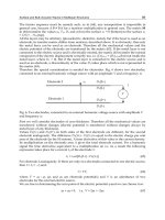
In Fig. 6 we present the overall development of concentration and deposition of SO
x
and
NOx and NHy in the Arctic since 1860, based on DEHM model runs and emission climate
data as described earlier. The patterns for NHy and NOx are very similar to each other. It is

not clear why concentrations and deposition do not have exactly the same development, but
changes in temperature and precipitation patterns will influence the historical deposition
development. This development with an accelarating depositon during the 19
th
century and
a decline after about 1980, corresponds well with ice core observations such as Weiler et al.,
2005.


4. Climate change impact on future atmospheric nitrogen deposition in a
temperate climate
4.1 Background
Climate change, with increased air temperatures and changed precipitation patterns, is likely to
affect the biogeochemical nitrogen (N) cycle in northwestern Europe significantly (deWit et al.,
2008). The >40 years of historical weather data (ERA40) and dynamically downscaled climate
scenarios for Europe to the year 2100 have been used to assess the linkage between climate
variability and N deposition by means of the MATCH (Multi-scale Atmospheric Transport and
Chemistry) model (Hole & Enghardt, 2008).
Total nitrate (NO
3
)and total ammonium (NH
4
) concentrations in precipitation decreased
significantly at the Swedish EMEP stations from the mid 1980s to 2000 (Lövblad et al., 2004).
During the same period the pH of precipitation increased from ~4.2 to 4.6. Data from the national
throughfall network (Nettelblad et al., 2005) measurements of air- and precipitation chemistry at
around 100 sites across Sweden confirm the downward trend in concentrations of NO
3
and NH
4

in rain. The trend was particularly pronounced in southern Sweden. Due to increasing
precipitation amounts during the same period, however, the total deposition of reactive nitrogen
(NO
3
and NH
4
) has not decreased; instead it has remained roughly unchanged.
Increasing precipitation in a region will obviously result in increasing wet deposition if
atmospheric N concentrations are unchanged. Altered precipitation patterns and temperatures
are also likely to affect mobilisation of N pools in the soil and runoff to rivers, lakes and fjords (de
Wit et al., 2008). Since many aquatic ecosystems in Scandinavia are N limited, increasing N
fertilization will disturb the natural biological activity.
In the following we focus on future N deposition in northern Europe (Fennoscandia and the
Baltic countries) as a result of future climate change. There are substantial regional differences in
factors such as topography, annual mean temperature and precipitation in this area, and hence a
regional discussion is required. Our purposes are to examine (1) regional and seasonal
differences in climate change effects on nitrogen deposition, (2) whether changes in wet
deposition are proportional to changes in precipitation, and (3) the distribution between dry and
wet deposition. The MATCH model and the experimental set-up applied is described in Hole &
Enghardt (2008) and references therein.

4.2 Deposition in future climate – comparison with current climate
Figures 7 and 8 show the calculated relative change in annual mean deposition of NO
y
and NH
x

over northern Europe. The figures display the difference of the 30-year mean of annually
accumulated deposition during a future 30-year period minus the 30-year period labelled

“current climate” normalised by the “current climate”.
The Norwegian coast will experience a large increase in total N deposition due to increased
precipitation projected by the present climate change scenario (ECHAM4/OPYC3–RCA3, SRES
A2). The changes are most likely connected to the projected changes in precipitation in northern
Europe. On an annual basis the whole of Fennoscandia is expected to receive more precipitation
in 2071-2100 compared to “current climate”.
The deposition of NO
y
and NH
x
display similar increasing trends along the coast of Norway. In
northern Fennoscandia and in parts of southeast Sweden NH
x
decreases, while NO
y
is projected
to increase. East and south of the Baltic Sea, the increase in NH
x
deposition is much smaller than
the increase in NO
y
deposition. This is mostly because scavenging of NH
x
is more effective in
Inuence of climate variability on reactive nitrogen deposition in temperate and Arctic climate 109
The level of the monthly SO
4
2-
concentration in the beginning of the monitoring period is
higher than at the end of the period but there is not a significant trend at all of the stations.

For the NO
3
-
concentration, values are on the contrary higher during the winter months than
during the summer months (Hole et al. (2009)). The inter annual variation in the NO
3
-

concentration is larger than in the sulphate concentration. The level of the nitrate
concentration at the end of the monitoring period is lower than in the beginning at only the
Pinega station. At the Jäniskoski station, the concentration has increased during the winter
months. There are increasing trends in sulphate in precipitation at Ust-Moma in east Siberia
in winter but at this station background concentrations are very low. This could be due to
changes in Norilsk (NE Siberia, 69°21’ N 88°12’ E) emission or variability in transport
pattern (Hole et al., 2006b). However, Norilsk emissions are not well quantified, so no clear
conclusions can be drawn.
SO
4
2-
concentrations measured in air at monitoring stations in the High Arctic (Alert,
Canada; and Zeppelin, Svalbard) and at several monitoring stations in subarctic areas of
Fennoscandia and northwestern Russia show decreasing trends since the 1990s, which
corresponds well with Quinn et al. (2007). At many stations there are significant downward
trends for SO
4
2-
and SO
2
in air, both summer and winter. There are significant reductions of
SO

2
in Svanvik probably because emissions in the area are strongly reduced. For the air
concentration of the nitrogen compounds there is no clear pattern, but it is interesting to see
a positive trend in summer total NO
3
-
concentration at 3 stations. Total ammonium in air
also has both positive and negative trends in summer.

3.5 Historical and expected trends 2000-2030 with “constant” climate
The DEHM model with extensive chemistry has been run with two different emissions
scenarios: The “Business As Usual” (BAU) and the “Maximum technically Feasible
Reduction” (MFR), as described in in Hole et al. (2006b). For each emission scenario the
DEHM model has been run for the same meteorological input for the period 1991-1993 in
order to reduce the meteorological variations of the model results. The pollution penetrates
further north in the eastern Arctic compared to the western Arctic. This is in accordance
with Stohl (2006) and Iversen and Jordanger (1985) and is a result of differences in
circulation patterns and higher temperatures in the Barents sea region which allows air
masses from temperate regions to move to higher latitudes without being lifted.
In Fig. 6 we present the overall development of concentration and deposition of SO
x
and
NOx and NHy in the Arctic since 1860, based on DEHM model runs and emission climate
data as described earlier. The patterns for NHy and NOx are very similar to each other. It is
not clear why concentrations and deposition do not have exactly the same development, but
changes in temperature and precipitation patterns will influence the historical deposition
development. This development with an accelarating depositon during the 19
th
century and
a decline after about 1980, corresponds well with ice core observations such as Weiler et al.,

2005.


4. Climate change impact on future atmospheric nitrogen deposition in a
temperate climate
4.1 Background
Climate change, with increased air temperatures and changed precipitation patterns, is likely to
affect the biogeochemical nitrogen (N) cycle in northwestern Europe significantly (deWit et al.,
2008). The >40 years of historical weather data (ERA40) and dynamically downscaled climate
scenarios for Europe to the year 2100 have been used to assess the linkage between climate
variability and N deposition by means of the MATCH (Multi-scale Atmospheric Transport and
Chemistry) model (Hole & Enghardt, 2008).
Total nitrate (NO
3
)and total ammonium (NH
4
) concentrations in precipitation decreased
significantly at the Swedish EMEP stations from the mid 1980s to 2000 (Lövblad et al., 2004).
During the same period the pH of precipitation increased from ~4.2 to 4.6. Data from the national
throughfall network (Nettelblad et al., 2005) measurements of air- and precipitation chemistry at
around 100 sites across Sweden confirm the downward trend in concentrations of NO
3
and NH
4

in rain. The trend was particularly pronounced in southern Sweden. Due to increasing
precipitation amounts during the same period, however, the total deposition of reactive nitrogen
(NO
3
and NH

4
) has not decreased; instead it has remained roughly unchanged.
Increasing precipitation in a region will obviously result in increasing wet deposition if
atmospheric N concentrations are unchanged. Altered precipitation patterns and temperatures
are also likely to affect mobilisation of N pools in the soil and runoff to rivers, lakes and fjords (de
Wit et al., 2008). Since many aquatic ecosystems in Scandinavia are N limited, increasing N
fertilization will disturb the natural biological activity.
In the following we focus on future N deposition in northern Europe (Fennoscandia and the
Baltic countries) as a result of future climate change. There are substantial regional differences in
factors such as topography, annual mean temperature and precipitation in this area, and hence a
regional discussion is required. Our purposes are to examine (1) regional and seasonal
differences in climate change effects on nitrogen deposition, (2) whether changes in wet
deposition are proportional to changes in precipitation, and (3) the distribution between dry and
wet deposition. The MATCH model and the experimental set-up applied is described in Hole &
Enghardt (2008) and references therein.

4.2 Deposition in future climate – comparison with current climate
Figures 7 and 8 show the calculated relative change in annual mean deposition of NO
y
and NH
x

over northern Europe. The figures display the difference of the 30-year mean of annually
accumulated deposition during a future 30-year period minus the 30-year period labelled
“current climate” normalised by the “current climate”.
The Norwegian coast will experience a large increase in total N deposition due to increased
precipitation projected by the present climate change scenario (ECHAM4/OPYC3–RCA3, SRES
A2). The changes are most likely connected to the projected changes in precipitation in northern
Europe. On an annual basis the whole of Fennoscandia is expected to receive more precipitation
in 2071-2100 compared to “current climate”.

The deposition of NO
y
and NH
x
display similar increasing trends along the coast of Norway. In
northern Fennoscandia and in parts of southeast Sweden NH
x
decreases, while NO
y
is projected
to increase. East and south of the Baltic Sea, the increase in NH
x
deposition is much smaller than
the increase in NO
y
deposition. This is mostly because scavenging of NH
x
is more effective in
Climate Change and Variability110
source areas than scavenging of NO
y
.


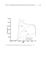
Fig. 7. Relative change in annually accumulated deposition of oxidised nitrogen (NO
y
) from
the period 1961-1990 to 2021-2050 (top row) and from 1961-1990 to 2071-2100 (bottom row).
Left panel is total deposition, middle panel is wet deposition, right panel is dry deposition.

Fig. 8. Same as Fig. 7, but for reduced nitrogen (NH
x
).
The total deposition of NO
y
over Norway is expected to increase from 96 Gg N year
-1
during
current climate to 107 Gg N year
-1
by the year 2100 due only to changes in climate (Hole &
Enghardt, 2008). The corresponding values for Sweden are more modest, 137 Gg N year
-1
to
139 Gg N year
-1
. Finland, the Baltic countries, Poland and Denmark will also experience
increases in total NO
y
deposition. A large part of the increase in total NO
y
deposition south
and east of the Baltic is due to increased dry deposition. Reduced precipitation and
increased atmospheric lifetimes of NO
y
results in higher surface concentrations here, which
drive up the dry deposition. In Norway and Sweden the change in annual dry deposition
from current to future climate is only minor and virtually all change in total NO
y
deposition

emanates from changes in wet deposition.
The total deposition of NH
x
decreases marginally in many countries around the Baltic Sea.
Decreasing wet deposition of NH
x
causes the decrease in total deposition in Sweden, Poland
and Denmark. Norway will experience a moderate increase in total NH
x
deposition in both
during 2021-2050 and 2071-2100 compared to “current climate” (52 Gg N year
-1
and 53 Gg N
year
-1
compared to 50 Gg N year
-1
).
Trends in deposition pattern for the two compounds are not identical because primary
emissions occur in different parts of Europe and because their deposition pathways differ.
NH
x
generally has a shorter atmospheric lifetime than NO
y
; the increased scavenging over
the coast of Norway will leave very little NH
x
to be deposited in northern Finland and the
Kola Peninsula, where NH
x

emissions are minor.
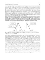
The relative increase in deposition is slightly smaller than the predicted increase in
precipitation. In Fig. 9 this dilution effect for NO
y
is apparent along the Norwegian coast
(where precipitation will increase most), but further north and east it is stronger because
much of the NO
y
is scavenged out before it reaches these areas.



Fig. 9. Relative change in concentration of oxidised nitrogen in precipitation from the period
1961-1990 to 2021-2050 (left) and from 1961-1990 to 2071-2100 (right).
Inuence of climate variability on reactive nitrogen deposition in temperate and Arctic climate 111
source areas than scavenging of NO
y
.


Fig. 7. Relative change in annually accumulated deposition of oxidised nitrogen (NO
y
) from
the period 1961-1990 to 2021-2050 (top row) and from 1961-1990 to 2071-2100 (bottom row).
Left panel is total deposition, middle panel is wet deposition, right panel is dry deposition.

Fig. 8. Same as Fig. 7, but for reduced nitrogen (NH
x
).
The total deposition of NO

y
over Norway is expected to increase from 96 Gg N year
-1
during
current climate to 107 Gg N year
-1
by the year 2100 due only to changes in climate (Hole &
Enghardt, 2008). The corresponding values for Sweden are more modest, 137 Gg N year
-1
to
139 Gg N year
-1
. Finland, the Baltic countries, Poland and Denmark will also experience
increases in total NO
y
deposition. A large part of the increase in total NO
y
deposition south
and east of the Baltic is due to increased dry deposition. Reduced precipitation and
increased atmospheric lifetimes of NO
y
results in higher surface concentrations here, which
drive up the dry deposition. In Norway and Sweden the change in annual dry deposition
from current to future climate is only minor and virtually all change in total NO
y
deposition
emanates from changes in wet deposition.
The total deposition of NH
x
decreases marginally in many countries around the Baltic Sea.

Decreasing wet deposition of NH
x
causes the decrease in total deposition in Sweden, Poland
and Denmark. Norway will experience a moderate increase in total NH
x
deposition in both
during 2021-2050 and 2071-2100 compared to “current climate” (52 Gg N year
-1
and 53 Gg N
year
-1
compared to 50 Gg N year
-1
).
Trends in deposition pattern for the two compounds are not identical because primary
emissions occur in different parts of Europe and because their deposition pathways differ.
NH
x
generally has a shorter atmospheric lifetime than NO
y
; the increased scavenging over
the coast of Norway will leave very little NH
x
to be deposited in northern Finland and the
Kola Peninsula, where NH
x
emissions are minor.
The relative increase in deposition is slightly smaller than the predicted increase in
precipitation. In Fig. 9 this dilution effect for NO
y

is apparent along the Norwegian coast
(where precipitation will increase most), but further north and east it is stronger because
much of the NO
y
is scavenged out before it reaches these areas.



Fig. 9. Relative change in concentration of oxidised nitrogen in precipitation from the period
1961-1990 to 2021-2050 (left) and from 1961-1990 to 2071-2100 (right).
Climate Change and Variability112
4.3 What can we say from these model results?
The accuracy of our results is determined by the accuracy of the utilised models and the
input to the models. MATCH has been used in a number of previous studies and has proven
capable to realistically simulate most species of interest. The model has, however, always
had limitations in its capability to simulate NH
x
species. This we have attributed to
relatively larger uncertainties in the emission inventory of NH
3
and to the fact that subgrid
emission/deposition processes not fully resolved in the system.
The model (RCA3) used to create the meteorological data in the present study has been
evaluated in Kjellström et al. (2005). Using observed meteorology (ERA40 from ECMWF;
“perfect boundary condition”) on the boundaries they compare the model output with
observations from a number of different sources. The increase in resolution from ERA40
produces precipitation fields more in line with observations although many topographical
and coastal effects are still not resolved. This could explain the underestimation of
precipitation at the sites located in western Norway. The precipitation in northern Europe is
also generally overestimated in RCA3 when ECHAM4/OPYC3 is used on its boundaries.

The degree of certainty we can attribute to RCA3’s predictions of future climate is not only
dependent on the climate model’s ability to describe “current climate” and how the regional
climate will respond to the increased greenhouse gas forcing. The RCA3 results are to a
large degree forced by the boundary data from the global climate model. The EU project
PRUDENCE and BALTEX presented a wide range of possible down-scaled scenarios for
northwestern Europe showing, for example, that winter precipitation can increase by 20 to
60% in Scandinavia (see (Christensen et al., 2007) and references therein). These
uncertainties are thus of the same order of magnitude as the projected changes in N
deposition.
Estimates of precursor (NO
X
, VOCs, CO etc.) emission strengths comprise a large
uncertainty when assessing future N deposition. In order to only study the impact that
possible climate changes may have on the deposition of N species we have kept emissions at
their 2000-levels. This is a simplification and future N loading in north-western Europe will
also be affected by changes in Europe as well as America and Asia. This study has focussed
on the change in N deposition due to climate change and not evaluated the relative
importance of altered precursor emissions or changed inter-hemispheric transport. The
change in deposition over an area may not always be the result of changes in the driving
meteorology over that area. It can of course also be due to changes in atmospheric transport
pathways or deposition en route to the area under consideration.

5. Discussion and conclusions
In section 2 we studied observations of N deposition and its relation to climate variability.
We showed that 36 % of the variation in winter nitrate wet deposition is described by the
North Atlantic Oscillation Index in coastal stations, while deposition at the inland station
Langtjern seems to be more controlled by the European blocking index. The Arctic
Oscillation Index gives good correlation at the northernmost station in addition to the
coastal (western) stations. Local air temperature is highly correlated (R=0.84) with winter
nitrate deposition at the western stations, suggesting that warm, humid winter weather

results in high wet deposition. For concentrations the best correlation was found for the
coastal station Haukeland in winter (R=-0.45). In addition, there was a tendency in the data
that high precipitation resulted in lower Nr concentrations. Removing trends in the data did
not have significant influence on the correlations observed. However, a careful sector
analysis for each month and for each station could improve the understanding of the
separate effects of emission variability and climate variability on the deposition.
For the Business as Usual (BAU) emission scenarios, northern hemisphere sulphur
emissions will only decline from 52.3 mt to 51.3 mt from 2000 to 2020 (section 3). For the
Most Feasible Reduction (MFR) scenario 2020 emissions will be only 20.2 mt. However, the
two different scenarios show much smaller differences in concentration and deposition of
sulphur in the Arctic. This is because the largest potential for improvement in SO
2
emissions
is in China and SE Asia. These regions have little influence on Arctic pollution according to
Stohl (2006) and others. For oxidized and reduced nitrogen compounds there is more
reduction in the emissions in Russia and Europe in the MFR scenario, and hence the
potential for improvement in the Arctic is larger.
SO
4
2-
concentrations are decreasing significantly at many Arctic stations. For NO
3
-
and NH
4
+

the pattern is unclear (some positive and some negative trends). There are few signs of
significant trends in precipitation for the period studied here (last 3 decades). However,
expected future occurrence of rain events in both summer and winter can result in

increasing wet deposition in the Arctic (ACIA, 2004, www.amap.no/acia).
There is relatively good monitoring data coverage in Fennoscandia and on Kola peninsula in
Russia, but there are otherwise few stations for background air and precipitation
concentration measurements in the Arctic. In our observations there are few differences
between summer and winter observations, although NO
3
-
wet deposition is higher in winter
in some stations in NW Russia and Fennoscandia (Pinega, Oulanka, Bredkal and Karasjok).
The explanation for this is not clear, but in Hole et al (2006b) seasonal exposure differences
for SO
2
at Oulanka are revealed which can indicate that transport path differences are part
of the explanation for the seasonal pattern.
Because of new technologies and climate change, future emissions and deposition are
particularly uncertain due to the expected increase in human activities in the polar and sub-
polar regions. Increased extraction of natural resources and increased sea traffic can be
expected. Climate change is also likely to influence transport and deposition patterns
(ACIA, 2004, www.amap.no/acia). There is a need for a deeper insight in plans and
consequences with respect to the Arctic. Modelling results presented here seem to rule out
SE Asia as an important contributor to pollution close to the surface in the Arctic
atmosphere. This is in accordance with earlier studies (e.g. Iversen and Jordanger, 1985,
Stohl, 2006) giving thermodynamic arguments why SE Asian emissions will have minor
influence in the Arctic.
As for the relation between future Nr deposition and climate scenarios in temperate climate
(section 4), our results suggest that prediction of future Nr deposition for different climate
scenarios most of all need good predictions of precipitation amount and precipitation
distribution in space and time. Climate indices can be a tool to understand this connection.
Regional differences in the expected changes are large. This is due to expected large increase
in precipitation along the Norwegian coast, while other areas can expect much smaller

changes. Country-averaged changes are moderate. Wet deposition will increase relatively
less than precipitation because of dilution. In Norway the contribution from dry deposition
will be relatively reduced because most of the N will be effectively removed by wet
deposition. In the Baltic countries both wet and dry deposition will increase. Dry deposition
Inuence of climate variability on reactive nitrogen deposition in temperate and Arctic climate 113
4.3 What can we say from these model results?
The accuracy of our results is determined by the accuracy of the utilised models and the
input to the models. MATCH has been used in a number of previous studies and has proven
capable to realistically simulate most species of interest. The model has, however, always
had limitations in its capability to simulate NH
x
species. This we have attributed to
relatively larger uncertainties in the emission inventory of NH
3
and to the fact that subgrid
emission/deposition processes not fully resolved in the system.
The model (RCA3) used to create the meteorological data in the present study has been
evaluated in Kjellström et al. (2005). Using observed meteorology (ERA40 from ECMWF;
“perfect boundary condition”) on the boundaries they compare the model output with
observations from a number of different sources. The increase in resolution from ERA40
produces precipitation fields more in line with observations although many topographical
and coastal effects are still not resolved. This could explain the underestimation of
precipitation at the sites located in western Norway. The precipitation in northern Europe is
also generally overestimated in RCA3 when ECHAM4/OPYC3 is used on its boundaries.
The degree of certainty we can attribute to RCA3’s predictions of future climate is not only
dependent on the climate model’s ability to describe “current climate” and how the regional
climate will respond to the increased greenhouse gas forcing. The RCA3 results are to a
large degree forced by the boundary data from the global climate model. The EU project
PRUDENCE and BALTEX presented a wide range of possible down-scaled scenarios for
northwestern Europe showing, for example, that winter precipitation can increase by 20 to

60% in Scandinavia (see (Christensen et al., 2007) and references therein). These
uncertainties are thus of the same order of magnitude as the projected changes in N
deposition.
Estimates of precursor (NO
X
, VOCs, CO etc.) emission strengths comprise a large
uncertainty when assessing future N deposition. In order to only study the impact that
possible climate changes may have on the deposition of N species we have kept emissions at
their 2000-levels. This is a simplification and future N loading in north-western Europe will
also be affected by changes in Europe as well as America and Asia. This study has focussed
on the change in N deposition due to climate change and not evaluated the relative
importance of altered precursor emissions or changed inter-hemispheric transport. The
change in deposition over an area may not always be the result of changes in the driving
meteorology over that area. It can of course also be due to changes in atmospheric transport
pathways or deposition en route to the area under consideration.

5. Discussion and conclusions
In section 2 we studied observations of N deposition and its relation to climate variability.
We showed that 36 % of the variation in winter nitrate wet deposition is described by the
North Atlantic Oscillation Index in coastal stations, while deposition at the inland station
Langtjern seems to be more controlled by the European blocking index. The Arctic
Oscillation Index gives good correlation at the northernmost station in addition to the
coastal (western) stations. Local air temperature is highly correlated (R=0.84) with winter
nitrate deposition at the western stations, suggesting that warm, humid winter weather
results in high wet deposition. For concentrations the best correlation was found for the
coastal station Haukeland in winter (R=-0.45). In addition, there was a tendency in the data
that high precipitation resulted in lower Nr concentrations. Removing trends in the data did
not have significant influence on the correlations observed. However, a careful sector
analysis for each month and for each station could improve the understanding of the
separate effects of emission variability and climate variability on the deposition.

For the Business as Usual (BAU) emission scenarios, northern hemisphere sulphur
emissions will only decline from 52.3 mt to 51.3 mt from 2000 to 2020 (section 3). For the
Most Feasible Reduction (MFR) scenario 2020 emissions will be only 20.2 mt. However, the
two different scenarios show much smaller differences in concentration and deposition of
sulphur in the Arctic. This is because the largest potential for improvement in SO
2
emissions
is in China and SE Asia. These regions have little influence on Arctic pollution according to
Stohl (2006) and others. For oxidized and reduced nitrogen compounds there is more
reduction in the emissions in Russia and Europe in the MFR scenario, and hence the
potential for improvement in the Arctic is larger.
SO
4
2-
concentrations are decreasing significantly at many Arctic stations. For NO
3
-
and NH
4
+

the pattern is unclear (some positive and some negative trends). There are few signs of
significant trends in precipitation for the period studied here (last 3 decades). However,
expected future occurrence of rain events in both summer and winter can result in
increasing wet deposition in the Arctic (ACIA, 2004, www.amap.no/acia).
There is relatively good monitoring data coverage in Fennoscandia and on Kola peninsula in
Russia, but there are otherwise few stations for background air and precipitation
concentration measurements in the Arctic. In our observations there are few differences
between summer and winter observations, although NO
3

-
wet deposition is higher in winter
in some stations in NW Russia and Fennoscandia (Pinega, Oulanka, Bredkal and Karasjok).
The explanation for this is not clear, but in Hole et al (2006b) seasonal exposure differences
for SO
2
at Oulanka are revealed which can indicate that transport path differences are part
of the explanation for the seasonal pattern.
Because of new technologies and climate change, future emissions and deposition are
particularly uncertain due to the expected increase in human activities in the polar and sub-
polar regions. Increased extraction of natural resources and increased sea traffic can be
expected. Climate change is also likely to influence transport and deposition patterns
(ACIA, 2004, www.amap.no/acia). There is a need for a deeper insight in plans and
consequences with respect to the Arctic. Modelling results presented here seem to rule out
SE Asia as an important contributor to pollution close to the surface in the Arctic
atmosphere. This is in accordance with earlier studies (e.g. Iversen and Jordanger, 1985,
Stohl, 2006) giving thermodynamic arguments why SE Asian emissions will have minor
influence in the Arctic.
As for the relation between future Nr deposition and climate scenarios in temperate climate
(section 4), our results suggest that prediction of future Nr deposition for different climate
scenarios most of all need good predictions of precipitation amount and precipitation
distribution in space and time. Climate indices can be a tool to understand this connection.
Regional differences in the expected changes are large. This is due to expected large increase
in precipitation along the Norwegian coast, while other areas can expect much smaller
changes. Country-averaged changes are moderate. Wet deposition will increase relatively
less than precipitation because of dilution. In Norway the contribution from dry deposition
will be relatively reduced because most of the N will be effectively removed by wet
deposition. In the Baltic countries both wet and dry deposition will increase. Dry deposition
Climate Change and Variability114
will increase here probably because of increased occurrence of wet surfaces.

According to our model results, northwestern Europe will generally experience small
changes in N deposition as a consequence of climate change. The exception is the west coast
of Norway, which will experience an increase in N deposition of 10-20% in the period 2021-
2050 and 20-40% in 2071-2100 (compared to current climate). Although Norway as a whole
will only experience a moderate increase in N deposition of about 10%, there are large
regional differences. RCA3/MATCH forced by ECHAM4/OPYC3 (SRES A2) prescribes
that a large part of the Norwegian coast is expected to receive at least 50% increase of the
precipitation during the period 2071-2100 compared to period 1961-1990, which is in line
with other regional climate scenarios. This region has already experienced increasing
precipitation in recent decades. The total effect on soil and watercourse chemistry of the
dramatic change in these regions remains to be thoroughly understood.
Our studies shows that expected reduction in future N deposition (as a consequence of
emission reductions in Europe) could be partly offset due to increasing precipitation in some
regions in the coming century. Future long term N emissions in Europe are difficult to
predict, however, since they depend on highly uncertain factors such as the future use of
fossil fuels and farming technology. The same uncertainty obviously also applies to the
greenhouse gas emission scenarios.

6. References
Aas, W.; Solberg, S.; Berg, T.; Manø, S. & Yttri, K. E. (2006). Monitoring of long range
transported pollution in Norway. Atmospheric transport, 2005. (In Norwegian).
Norwegian Pollution Control Authority. Rapport 955/2006. TA-2180/2006. NILU OR
36/2006. www.nilu.no.

Barrie L.A., 1986. Arctic air pollution: An overview of current knowledge. Atm. Env. 20, 643-663.
Barrie, L.A.; Fisher, D. & Koerner, R.M. (2005). Twentieth century trends in Arctic air
pollution revealed by conductivity and acidity observations in snow and ice in the
Canadian High Arctic. Atmospheric Environment, 19 (12), 2055-2063.
Bobbink, R.; Hornung, M. & Roelofs, J.G.M. (1998). The effects of air-borne nitrogen
pollutants on species diversity in natural and semi-natural European vegetation.

Journal Of Ecology 86(5): 717-738.
Christensen, J. (1997). The Danish Eulerian Hemispheric Model - A Three Dimensional Air
Pollution Model Used for the Arctic. Atm. Env, 31, 4169-4191.
Christensen, J.H.; Carter, T.R.; Rummukainen M. & Amanatidis, G. (2007). Evaluating the
performance and utility of climate models: the PRUDENCE project. Climatic
Change, Vol 81. doi:10.1007/s10584-006-9211-6.
de Wit, H.A.; Hindar, A. & Hole, L. (2008). Winter climate affects long-term trends in
streamwater nitrate in acid-sensitive catchments in southern Norway. Hydrology
and Earth System Sciences, 12, 393-403.
Delwiche, C. C. (1970). The nitrogen cycle. Sci. Am. 223: 137-146, 1970.
EMEP (2006). Transboundary acidification, eutrophication and ground level ozone in
Europe since 1990 to 2004. EMEP Status Report1/2006. The Norwegian
Meteorological Institute, Oslo, EMEP/MSC-W Report 1/97
Flatøy, F. & Hov, Ø. (1996). Three-dimensional model studies of the effect of NOx emissions
from aircrafts on ozone in the upper troposphere over Europe and the North
Atlantic. J. Geophys. Res., 101, 1401-1422.
Fowler, D.; Smith, R. I.; Muller, J. B. A.; Hayman, G. & Vincent, K. J. (2006). Changes in the
atmospheric deposition of acidifying compounds in the UK between 1986 and 2001.
Env. Poll., 137(1): 15-25.
Frohn, L.M.; Christensen, J. H.; Brandt, J.; Geels, C. & Hansen, K. (2003). Validation of a 3-D
hemispheric nested air pollution model. Atmospheric Chemistry and Physics, 3,3543-3588
Frohn, L.M.; Christensen, J. H. & Brandt, J., (2002). Development and testing of numerical
methods for two-way nested air pollution modelling. Physics and Chemistry of the
Earth, Parts A/B/C, 27 (35), P. 1487-1494
Galloway, J. N.; Dentener, F. J.; Capone, D. G.; Boyer, E. W.; Howarth, R. W.; Seitzinger, S.
P.; Asner, G. P.; Cleveland, C.; Green, P.; Holland, E.; Karl, D. M.; Michaels, A. F.;
Porter, J. H. Townsend, A. & Vörösmarty, C. (2004). Nitrogen Cycles: Past, Present
and Future. Biogeochemistry 70: 153-226.
Geels, C.; Doney, S.C.; Dargaville, R. J. Brandt, J.; Christensen, J.H. (2004). Investigating the
sources of synoptic variability in atmospheric CO2 measurements over the

Northern Hemisphere continents: a regional model study. Tellus B 56 (1), 35–50.
doi:10.1111/j.1600-0889.2004.00084.x
Gilbert, R. O.: Statistical methods for environmental pollution monitoring. Van Nostrand
Reinhold , New York, 1987.
Grell, G.; J. Dudhia, and Stauffer, D. (1994). A description of the Fifth-Generation Penn
State/NCAR Mesoscale Model (MM5), NCAR Tech. Note TN-398, Natl. Cent. for
Atmos. Res., Boulder, Colo
Hansen, K.M.; Christensen, J.H.; Brandt, J.; Frohn, L.M.; & Geels, C.(2004). Modelling
atmospheric transport of α-hexachlorocyclohexane in the Northern Hemispherewith a
3-D dynamical model: DEHM-POP, Atmos. Chem. Phys., 4, 1125-1137.
Hanssen-Bauer, I. (2005). Regional temperature and precipitation series for Norway:
Analyses of time-series updated to 2004. Met.no report 15/2005.
Heidam, N.Z.; Christensen, J.; Wåhlin, P. & Skov, H. (2004). Arctic atmospheric
contaminants in NE Greenland: levels, variations, origins, transport,
transformations and trends 1990–2001 Science of The Total Environment, 331 (1-3).
Pages 5-28.
Hertel, O.; Christensen, J.; Runge, E.H.; Asman, W.A.H.; Berkowicz, R.& Hovmand, M.F.
(1995). Development and Testing of a new Variable Scale Air Pollution Model -
ACDEP. Atmospheric Environment, 29 1267-1290.
Hole, L. R. & Tørseth, K. (2002). Deposition of major inorganic compounds in Norway 1978-
1982 and 1997-2001: status and trends. Naturens tålegrenser. Norwegian Pollution
Control Authority. Report 115. NILU OR 61/2002, ISBN: 82-425-1410-0.
www.nilu.no , 2002.
Hole, L.R, Christensen, J.; Ruoho-Airola, T.; Wilson, S.; Ginzburg, V. A.; Vasilenko, V.N.;
Polishok, A.I. & Stohl, A.I. (2006). Acidifying pollutants, Arctic Haze and Acidification
in the Arctic. AMAP assessment report 2006, ch. 3, pp 11-31.
Hole, L.R. & Engardt, M.; (2008) . Climate change impact on atmospheric nitrogen
deposition in northwestern Europe – a model study. AMBIO 37 (1), 9-17.
Inuence of climate variability on reactive nitrogen deposition in temperate and Arctic climate 115
will increase here probably because of increased occurrence of wet surfaces.

According to our model results, northwestern Europe will generally experience small
changes in N deposition as a consequence of climate change. The exception is the west coast
of Norway, which will experience an increase in N deposition of 10-20% in the period 2021-
2050 and 20-40% in 2071-2100 (compared to current climate). Although Norway as a whole
will only experience a moderate increase in N deposition of about 10%, there are large
regional differences. RCA3/MATCH forced by ECHAM4/OPYC3 (SRES A2) prescribes
that a large part of the Norwegian coast is expected to receive at least 50% increase of the
precipitation during the period 2071-2100 compared to period 1961-1990, which is in line
with other regional climate scenarios. This region has already experienced increasing
precipitation in recent decades. The total effect on soil and watercourse chemistry of the
dramatic change in these regions remains to be thoroughly understood.
Our studies shows that expected reduction in future N deposition (as a consequence of
emission reductions in Europe) could be partly offset due to increasing precipitation in some
regions in the coming century. Future long term N emissions in Europe are difficult to
predict, however, since they depend on highly uncertain factors such as the future use of
fossil fuels and farming technology. The same uncertainty obviously also applies to the
greenhouse gas emission scenarios.

6. References
Aas, W.; Solberg, S.; Berg, T.; Manø, S. & Yttri, K. E. (2006). Monitoring of long range
transported pollution in Norway. Atmospheric transport, 2005. (In Norwegian).
Norwegian Pollution Control Authority. Rapport 955/2006. TA-2180/2006. NILU OR
36/2006. www.nilu.no.
Barrie L.A., 1986. Arctic air pollution: An overview of current knowledge. Atm. Env. 20, 643-663.
Barrie, L.A.; Fisher, D. & Koerner, R.M. (2005). Twentieth century trends in Arctic air
pollution revealed by conductivity and acidity observations in snow and ice in the
Canadian High Arctic. Atmospheric Environment, 19 (12), 2055-2063.
Bobbink, R.; Hornung, M. & Roelofs, J.G.M. (1998). The effects of air-borne nitrogen
pollutants on species diversity in natural and semi-natural European vegetation.
Journal Of Ecology 86(5): 717-738.

Christensen, J. (1997). The Danish Eulerian Hemispheric Model - A Three Dimensional Air
Pollution Model Used for the Arctic. Atm. Env, 31, 4169-4191.
Christensen, J.H.; Carter, T.R.; Rummukainen M. & Amanatidis, G. (2007). Evaluating the
performance and utility of climate models: the PRUDENCE project. Climatic
Change, Vol 81. doi:10.1007/s10584-006-9211-6.
de Wit, H.A.; Hindar, A. & Hole, L. (2008). Winter climate affects long-term trends in
streamwater nitrate in acid-sensitive catchments in southern Norway. Hydrology
and Earth System Sciences, 12, 393-403.
Delwiche, C. C. (1970). The nitrogen cycle. Sci. Am. 223: 137-146, 1970.
EMEP (2006). Transboundary acidification, eutrophication and ground level ozone in
Europe since 1990 to 2004. EMEP Status Report1/2006. The Norwegian
Meteorological Institute, Oslo, EMEP/MSC-W Report 1/97
Flatøy, F. & Hov, Ø. (1996). Three-dimensional model studies of the effect of NOx emissions
from aircrafts on ozone in the upper troposphere over Europe and the North
Atlantic. J. Geophys. Res., 101, 1401-1422.
Fowler, D.; Smith, R. I.; Muller, J. B. A.; Hayman, G. & Vincent, K. J. (2006). Changes in the
atmospheric deposition of acidifying compounds in the UK between 1986 and 2001.
Env. Poll., 137(1): 15-25.
Frohn, L.M.; Christensen, J. H.; Brandt, J.; Geels, C. & Hansen, K. (2003). Validation of a 3-D
hemispheric nested air pollution model. Atmospheric Chemistry and Physics, 3,3543-3588
Frohn, L.M.; Christensen, J. H. & Brandt, J., (2002). Development and testing of numerical
methods for two-way nested air pollution modelling. Physics and Chemistry of the
Earth, Parts A/B/C, 27 (35), P. 1487-1494
Galloway, J. N.; Dentener, F. J.; Capone, D. G.; Boyer, E. W.; Howarth, R. W.; Seitzinger, S.
P.; Asner, G. P.; Cleveland, C.; Green, P.; Holland, E.; Karl, D. M.; Michaels, A. F.;
Porter, J. H. Townsend, A. & Vörösmarty, C. (2004). Nitrogen Cycles: Past, Present
and Future. Biogeochemistry 70: 153-226.
Geels, C.; Doney, S.C.; Dargaville, R. J. Brandt, J.; Christensen, J.H. (2004). Investigating the
sources of synoptic variability in atmospheric CO2 measurements over the
Northern Hemisphere continents: a regional model study. Tellus B 56 (1), 35–50.

doi:10.1111/j.1600-0889.2004.00084.x
Gilbert, R. O.: Statistical methods for environmental pollution monitoring. Van Nostrand
Reinhold , New York, 1987.
Grell, G.; J. Dudhia, and Stauffer, D. (1994). A description of the Fifth-Generation Penn
State/NCAR Mesoscale Model (MM5), NCAR Tech. Note TN-398, Natl. Cent. for
Atmos. Res., Boulder, Colo
Hansen, K.M.; Christensen, J.H.; Brandt, J.; Frohn, L.M.; & Geels, C.(2004). Modelling
atmospheric transport of α-hexachlorocyclohexane in the Northern Hemispherewith a
3-D dynamical model: DEHM-POP, Atmos. Chem. Phys., 4, 1125-1137.
Hanssen-Bauer, I. (2005). Regional temperature and precipitation series for Norway:
Analyses of time-series updated to 2004. Met.no report 15/2005.
Heidam, N.Z.; Christensen, J.; Wåhlin, P. & Skov, H. (2004). Arctic atmospheric
contaminants in NE Greenland: levels, variations, origins, transport,
transformations and trends 1990–2001 Science of The Total Environment, 331 (1-3).
Pages 5-28.
Hertel, O.; Christensen, J.; Runge, E.H.; Asman, W.A.H.; Berkowicz, R.& Hovmand, M.F.
(1995). Development and Testing of a new Variable Scale Air Pollution Model -
ACDEP. Atmospheric Environment, 29 1267-1290.
Hole, L. R. & Tørseth, K. (2002). Deposition of major inorganic compounds in Norway 1978-
1982 and 1997-2001: status and trends. Naturens tålegrenser. Norwegian Pollution
Control Authority. Report 115. NILU OR 61/2002, ISBN: 82-425-1410-0.
www.nilu.no , 2002.
Hole, L.R, Christensen, J.; Ruoho-Airola, T.; Wilson, S.; Ginzburg, V. A.; Vasilenko, V.N.;
Polishok, A.I. & Stohl, A.I. (2006). Acidifying pollutants, Arctic Haze and Acidification
in the Arctic. AMAP assessment report 2006, ch. 3, pp 11-31.
Hole, L.R. & Engardt, M.; (2008) . Climate change impact on atmospheric nitrogen
deposition in northwestern Europe – a model study. AMBIO 37 (1), 9-17.
Climate Change and Variability116
Hole, L.R.; Brunner, S.H.; J.E. Hansen & L. Zhang, (2008). Low cost measurements of
nitrogen and sulphur dry deposition velocities at a semi-alpine site: Gradient

measurements and a comparison with deposition model estimates. Env. Poll., 154,
473-481. Special issue on biosphere-atmosphere fluxes, .
Hole, L.R.; Christensen, J. Forsius, M.; Nyman, M.; Stohl, A. & Wilson, S. (2006b). Sources of
acidifying pollutants and Arctic haze precursors. AMAP assessment report ,
chapter 2.
Hole, L.R.; de Wit, H.; & Aas, W. (2008). Trends in N deposition in Norway: A regional
perspective. Hydrology and Earth System Sciences 12, 405-414.
Iversen, T. & Jordanger, E. (2008). Arctic air pollution and large scale atmospheric flows,
Atm. Env., 19, 2099-2108.
Jonson, J.E. , Kylling, A. , Berntsen, T. , Isaksen, I.S.A. , Zerefos, C.S. , & Kourtidis, K. (2000),
Chemical effects of UV fluctuations inferred from total ozone and tropospheric
aerosol variations, J. Geophys. Res., 105, 14561-14574.
Kämäri, J. & Joki-Heiskala, P., (eds), (1998). AMAP assessment report ch. 9, 621-658.
Acidifying Pollutants, Arctic haze, and Acidification in the Arctic. Arctic Monitoring
and Assessment Programme, www.amap.no.
Kjellström, E.; Bärring, L.; Gollvik, S.; Hansson, U.; Jones, C.; Samuelsson, P.;
Rummukainen, M.; Ullerstig, A.; Willén, U. & Wyser, K. (2005). A 140-year
simulation of the European climate with the new version of the Rossby Centre regional
atmospheric climate model (RCA3). SMHI Reports Meteorology and Climatology No.
108, SMHI, SE-60176 Norrköping, Sweden 54 pp.
Kylling, A. , Bais, A.F. , Blumthaler, M. , Schreder, J. , Zerefos, C. S. , & Kosmidis, E. , (1998),
The effect of aerosols on solar UV irradiances during the Photochemical Activity
and Solar Radiation campaign, J. Geophys. Res., 103, 21051-26060
Langner, J.; Bergström, R. & Foltescu, V. (2005). Impact of climate change on surface ozone
and deposition of sulphur and nitrogen in Europe. Atm. Env., 39 (6), 1129-1141.
Levine S.Z. & Schwarz S.E.; (1982). In-cloud and below-cloud scavenging of nitric acid
vapor. Atm. Env. 16, 1725-1734.
Logan J.A.; (1983). Nitrogen oxides in the troposphere; global and regional budgets. J.
Geophys. Res. 88, 10785-10807.
Lövblad, G.; Henningsson, E.; Sjöberg, K.; Brorström-Lundén, E.; Lindskog, A. & Munthe, J.

(2004). Trends in Swedish background air 1980-2000. In: EMEP Assessment part II
National Contributions. (. pp. 211-220. Oslo ISBN-82-7144-032-2.
MacDonald, R.W.; Harner, T. and Fyfe, J. (2005). Recent climate change in the Arctic and its
impact on contaminant pathways and interpretation of temporal trend data. Sci.
Tot. Environ. 342, 5–86.
Nettelblad, A.; Westling, O.; Akselsson, C.; Svensson, A. & Hellsten, S. (2006). Air pollution at
forest sites – results until September 2005. (In Swedish). IVL Rapport B 1682. 50 pp. (In
Swedish).
Orsolini, Y. J. & Doblas-Reyes, F. J. (2002) Ozone signatures of climate patterns over the
Euro-Atlantic sector in the spring, Q. J. R. Meteorol. Soc., 129, 3251-3263.
Quinn PK, Shaw G, Andrews E, Dutton EG, Ruoho-Airola T, & Gong SL. (2007) Arctic haze:
current trends and knowledge gaps Tellus
B 59 (1): 99-114.
Salmi, T.; Määttä, A.; Anttila, P.; Ruoho-Airola, T. & Amnell, T. (2002). Detecting trends of
annual values of atmospheric pollutants by the Mann-Kendall test and Sen’s slope
estimates – the Excel template application MAKESENS, Publications on Air Quality,
no. 31, FMI-AQ-31, FMI, Helsinki, Finland.
Schwarz S.E. (1979). Residence times in reservoirs under non-steady-state conditions:
application to atmospheric SO2 and aerosol sulphate. Tellus 31, 520-547.
Seinfeld J.H. & Pandis S.N. (1998). Atmospheric Chemistry and Physics: From Air Pollution to
Climate Change, John Wiley & Sons, Inc., New York.
Sen P. K. (1968). Estimates of the regression coefficient based on Kendall’s tau. J. of the
American Statistical Association, 63, 1379-1389.
Simpson, D.; Fagerli, H.; Hellsten, S.; Knulst, K.; Westling, O. (2006). Comparison of
modelled and monitored deposition fluxes of sulphur and nitrogen to ICP-forest
sites in Europe. Biogeosciences 3, 337–355.
Stoddard, J. L. Long-Term Changes In Watershed Retention Of Nitrogen - Its Causes And
Aquatic Consequences (1994). Environmental Chemistry Of Lakes And Reservoirs. 237:
223-284.
Stohl, A. (2006). Characteristics of atmospheric transport into the Arctic troposphere. J.

Geophys. Res. 111, D11306, doi:10.1029/2005JD006888.
Sutton, M. A.; Asman, W. A. H.; Ellermann, T.; van Jaarsveld, J. A.; Acker, K.; Aneja, V.;
Duyzer, J.; Horvath, L.; Paramonov, S.; Mitosinkova, M.; Tang, Y. S.; Achtermann,
B.; Gauger, T.; Bartniki, J.; Neftel, A. and Erisma, J.W. (2003). Establishing the link
between ammonia emission control and measurements of reduced nitrogen
concentrations and deposition. Environ Monit. Asessm. 82:149-85.
Tietema, A.; A.W. Boxman, A.W.; Bredemeier M.; Emmett, B.A.; Moldan F.; Gundersen P.;
Schleppi P. & Wright R.F.: Nitrogen saturation experiments (NITREX) in
coniferous forest ecosystems in Europe: a summary of results. Environmental
Pollution 102: 433-437, 1998
Tørseth, K.; Aas, W. & Solberg, S. (2001). Trends in airborne sulphur and nitrogen
compounds in Norway during 1985-1996 in relation to airmass origin. Water, Air
and Soil. Poll. 130, 1493-1498
Weiler, K.; Fischer, H.; Fritzsche, Ruth, U.; Wilhelms, F. & Miller H. (2005). Glaciochemical
reconnaissance of a new ice core from Severnaya Zemlya, Eurasian Arctic. J.
Glaciology, Vol. 51, No. 172, 64-74.
Wesely M.L. & Hicks B.B. (2000). A review of the current status of knowledge on dry
deposition. Atm. Env. 34, 2261-2282.
Inuence of climate variability on reactive nitrogen deposition in temperate and Arctic climate 117
Hole, L.R.; Brunner, S.H.; J.E. Hansen & L. Zhang, (2008). Low cost measurements of
nitrogen and sulphur dry deposition velocities at a semi-alpine site: Gradient
measurements and a comparison with deposition model estimates. Env. Poll., 154,
473-481. Special issue on biosphere-atmosphere fluxes, .
Hole, L.R.; Christensen, J. Forsius, M.; Nyman, M.; Stohl, A. & Wilson, S. (2006b). Sources of
acidifying pollutants and Arctic haze precursors. AMAP assessment report ,
chapter 2.
Hole, L.R.; de Wit, H.; & Aas, W. (2008). Trends in N deposition in Norway: A regional
perspective. Hydrology and Earth System Sciences 12, 405-414.
Iversen, T. & Jordanger, E. (2008). Arctic air pollution and large scale atmospheric flows,
Atm. Env., 19, 2099-2108.

Jonson, J.E. , Kylling, A. , Berntsen, T. , Isaksen, I.S.A. , Zerefos, C.S. , & Kourtidis, K. (2000),
Chemical effects of UV fluctuations inferred from total ozone and tropospheric
aerosol variations, J. Geophys. Res., 105, 14561-14574.
Kämäri, J. & Joki-Heiskala, P., (eds), (1998). AMAP assessment report ch. 9, 621-658.
Acidifying Pollutants, Arctic haze, and Acidification in the Arctic. Arctic Monitoring
and Assessment Programme, www.amap.no.
Kjellström, E.; Bärring, L.; Gollvik, S.; Hansson, U.; Jones, C.; Samuelsson, P.;
Rummukainen, M.; Ullerstig, A.; Willén, U. & Wyser, K. (2005). A 140-year
simulation of the European climate with the new version of the Rossby Centre regional
atmospheric climate model (RCA3). SMHI Reports Meteorology and Climatology No.
108, SMHI, SE-60176 Norrköping, Sweden 54 pp.
Kylling, A. , Bais, A.F. , Blumthaler, M. , Schreder, J. , Zerefos, C. S. , & Kosmidis, E. , (1998),
The effect of aerosols on solar UV irradiances during the Photochemical Activity
and Solar Radiation campaign, J. Geophys. Res., 103, 21051-26060
Langner, J.; Bergström, R. & Foltescu, V. (2005). Impact of climate change on surface ozone
and deposition of sulphur and nitrogen in Europe. Atm. Env., 39 (6), 1129-1141.
Levine S.Z. & Schwarz S.E.; (1982). In-cloud and below-cloud scavenging of nitric acid
vapor. Atm. Env. 16, 1725-1734.
Logan J.A.; (1983). Nitrogen oxides in the troposphere; global and regional budgets. J.
Geophys. Res. 88, 10785-10807.
Lövblad, G.; Henningsson, E.; Sjöberg, K.; Brorström-Lundén, E.; Lindskog, A. & Munthe, J.
(2004). Trends in Swedish background air 1980-2000. In: EMEP Assessment part II
National Contributions. (. pp. 211-220. Oslo ISBN-82-7144-032-2.
MacDonald, R.W.; Harner, T. and Fyfe, J. (2005). Recent climate change in the Arctic and its
impact on contaminant pathways and interpretation of temporal trend data. Sci.
Tot. Environ. 342, 5–86.
Nettelblad, A.; Westling, O.; Akselsson, C.; Svensson, A. & Hellsten, S. (2006). Air pollution at
forest sites – results until September 2005. (In Swedish). IVL Rapport B 1682. 50 pp. (In
Swedish).
Orsolini, Y. J. & Doblas-Reyes, F. J. (2002) Ozone signatures of climate patterns over the

Euro-Atlantic sector in the spring, Q. J. R. Meteorol. Soc., 129, 3251-3263.
Quinn PK, Shaw G, Andrews E, Dutton EG, Ruoho-Airola T, & Gong SL. (2007) Arctic haze:
current trends and knowledge gaps Tellus
B 59 (1): 99-114.
Salmi, T.; Määttä, A.; Anttila, P.; Ruoho-Airola, T. & Amnell, T. (2002). Detecting trends of
annual values of atmospheric pollutants by the Mann-Kendall test and Sen’s slope
estimates – the Excel template application MAKESENS, Publications on Air Quality,
no. 31, FMI-AQ-31, FMI, Helsinki, Finland.
Schwarz S.E. (1979). Residence times in reservoirs under non-steady-state conditions:
application to atmospheric SO2 and aerosol sulphate. Tellus 31, 520-547.
Seinfeld J.H. & Pandis S.N. (1998). Atmospheric Chemistry and Physics: From Air Pollution to
Climate Change, John Wiley & Sons, Inc., New York.
Sen P. K. (1968). Estimates of the regression coefficient based on Kendall’s tau. J. of the
American Statistical Association, 63, 1379-1389.
Simpson, D.; Fagerli, H.; Hellsten, S.; Knulst, K.; Westling, O. (2006). Comparison of
modelled and monitored deposition fluxes of sulphur and nitrogen to ICP-forest
sites in Europe. Biogeosciences 3, 337–355.
Stoddard, J. L. Long-Term Changes In Watershed Retention Of Nitrogen - Its Causes And
Aquatic Consequences (1994). Environmental Chemistry Of Lakes And Reservoirs. 237:
223-284.
Stohl, A. (2006). Characteristics of atmospheric transport into the Arctic troposphere. J.
Geophys. Res. 111, D11306, doi:10.1029/2005JD006888.
Sutton, M. A.; Asman, W. A. H.; Ellermann, T.; van Jaarsveld, J. A.; Acker, K.; Aneja, V.;
Duyzer, J.; Horvath, L.; Paramonov, S.; Mitosinkova, M.; Tang, Y. S.; Achtermann,
B.; Gauger, T.; Bartniki, J.; Neftel, A. and Erisma, J.W. (2003). Establishing the link
between ammonia emission control and measurements of reduced nitrogen
concentrations and deposition. Environ Monit. Asessm. 82:149-85.
Tietema, A.; A.W. Boxman, A.W.; Bredemeier M.; Emmett, B.A.; Moldan F.; Gundersen P.;
Schleppi P. & Wright R.F.: Nitrogen saturation experiments (NITREX) in
coniferous forest ecosystems in Europe: a summary of results. Environmental

Pollution 102: 433-437, 1998
Tørseth, K.; Aas, W. & Solberg, S. (2001). Trends in airborne sulphur and nitrogen
compounds in Norway during 1985-1996 in relation to airmass origin. Water, Air
and Soil. Poll. 130, 1493-1498
Weiler, K.; Fischer, H.; Fritzsche, Ruth, U.; Wilhelms, F. & Miller H. (2005). Glaciochemical
reconnaissance of a new ice core from Severnaya Zemlya, Eurasian Arctic. J.
Glaciology, Vol. 51, No. 172, 64-74.
Wesely M.L. & Hicks B.B. (2000). A review of the current status of knowledge on dry
deposition. Atm. Env. 34, 2261-2282.
Climate Change and Variability118
Climate change: impacts on sheries and aquaculture 119
Climate change: impacts on sheries and aquaculture
Bimal P Mohanty, Sasmita Mohanty, Jyanendra K Sahoo and Anil P Sharma
x

Climate change: impacts on
fisheries and aquaculture

Bimal P Mohanty
1
, Sasmita Mohanty
2
,
Jyanendra K Sahoo
3
and Anil P Sharma
1
1
Central Inland Fisheries Research Institute, Barrackpore, Kolkata 700120;
2

School of Biotechnology,

KIIT University, Bhubaneswar 751024,
3
Orissa University of Agriculture & Technology, College of Fisheries, Berhampur760007;
India.

Climate change has been recognized as the foremost environmental problem of the twenty-
first century and has been a subject of considerable debate and controversy. It is predicted to
lead to adverse, irreversible impacts on the earth and the ecosystem as a whole. Although it
is difficult to connect specific weather events to climate change, increases in global
temperature has been predicted to cause broader changes, including glacial retreat, arctic
shrinkage and worldwide sea level rise. Climate change has been implicated in mass
mortalities of several aquatic species including plants, fish, corals and mammals. The
present chapter has been divided in to two parts; the first part discusses the causes and
general concerns of global climate change and the second part deals, specifically, on the
impacts of climate change on fisheries and aquaculture, possible mitigation options and
development of suitable monitoring tools.

1. Global Climate change: Causes and concerns
Climate change is the variation in the earth’s global climate or in regional climates over time
and it involves changes in the variability or average state of the atmosphere over durations
ranging from decades to millions of years. The United Nations Framework Convention on
Climate Change (UNFCCC) uses the term ‘climate change’ for human-caused change and
‘climate variability’ for other changes. In last 100 years, ending in 2005, the average global
air temperature near the earth’s surface has been estimated to increase at the rate of 0.74 +/-
0.18 °C (1.33 +/- 0.32 °F) (IPCC 2007). In recent usage, especially in the context of
environmental policy, the term ‘climate change’ often refers to changes in the modern
climate.

2. Causes of climate change
There are both natural processes and anthropogenic activities affecting the earth’s
temperature and the resultant climate change. The steep increases in the global
7
Climate Change and Variability120
anthropogenic greenhouse gas (GHG) emissions over the decades are major contributors to
the global warming.

2.1. Natural processes affecting the earth’s temperature
Sun is the primary source of energy on earth. Though the sun’s output is nearly constant,
small changes over an extended period of time can lead to climate change. The earth’s
climate changes are in response to many natural processes like orbital forcing (variations in
its orbit around the Sun), volcanic eruptions, and atmospheric greenhouse gas
concentrations. Changes in atmospheric concentrations of greenhouse gases and aerosols,
land-cover and solar radiation alter the energy balance of the climate system and causes
warming or cooling of the earth’s atmosphere. Volcanic eruptions emit many gases and one
of the most important of these is sulfur dioxide (SO
2
) which forms sulfate aerosol (SO
4
) in
the atmosphere.

2.2 Greenhouse gases
Greenhouse gases (GHGs) are those gaseous constituents of the atmosphere, both natural
and anthropogenic, that are responsible for the greenhouse effect, leading to an increase in
the amount of infrared or thermal radiation near the surface. While water vapor (H
2
O),
carbon dioxide (CO

2
), nitrous oxide (N
2
O), methane (CH
4
), and ozone (O
3
) are the primary
greenhouse gases in the Earth’s atmosphere, there are a number of entirely human-made
greenhouse gases in the atmosphere, such as the halocarbons and other chlorine- and
bromine-containing substances. Halocarbons such as CFCs (chlorofluorocarbons) are
completely artificial (man-made), and are produced from the chemical industry in which
they are used as coolants and in foam blowing.
Increases in CO
2
are the single largest factor contributing more than 60% of human-
enhanced increases and more than 90% of rapid increase in past decade. Most CO
2

emissions are from the burning of fossil fuels such as coal, oil, and gas. Rising CO
2
is also
related to deforestation, which eliminates an important carbon sink of the terrestrial
biosphere (www.ncdc.noaa.gov/oa/climate/globalwarming.html; Shea et al., 2007).
Currently, the atmosphere contains about 370 ppm of CO
2
, which is the highest
concentration in 420000 years and perhaps as long as 2 million years. Estimates of CO
2

concentrations at the end of the 21
st
century range from 490 to 1260 ppm, or a 75% to 350%
increase above preindustrial concentrations (WMO World Data Centre for Greenhouse
Gases. Greenhouse gas bulletin, 2006; Shea KM and the Committee on Environmental
Health, 2007)
.


3. Impacts of climate change
Although it is difficult to connect specific weather events to global warming, an increase in
global temperatures may in turn cause broader changes, including glacial retreat, arctic
shrinkage, and worldwide sea level rise. Changes in the amount and pattern of precipitation
may result in flooding and drought. Other effects may include changes in agricultural
yields, addition of new trade routes, reduced summer stream flows, species extinctions, and
increases in the range of disease vectors (Understanding and responding to Climate Change.
2008: ).
Most models on Global climate change indicate that snow pack is likely to decline on many
mountain ranges in the west, which would bring adverse impact on fish populations,
hydropower, water recreation and water availability for agricultural, industrial and
residential use. Partial loss of ice sheets on polar land could imply meters of sea level rise,
major changes in coastlines and inundation of low-lying areas, with greatest effects in river
deltas and low-lying islands. Such changes are projected to occur over millennial time
scales, but more rapid sea level rise on century time scales cannot be excluded. Current
models of climate change predict a rise in sea surface temperatures of between 2 °C and 5 °C
by the year 2100 (IPCC Third Assessment Report, 2001: Done et al., 2003).
Climate change will affect ecosystems and human systems like agricultural, transportation
and health infrastructure. The regions that will be most severely affected are often the
regions that are the least able to adept. Bangladesh is projected to lose 17.5 % of its land if
sea level rises about 1 meter (39 inches), displacing millions of people. Several islands in the

South Pacific and Indian oceans may disappear. Many other coastal regions will be at
increased risk of flooding, especially during storm surges, threatening animals, plants and
human infrastructure such as roads, bridges and water supplies.
There are many ways in which climate change might affect human health, including heat
stress, heat (sun) stroke, increased air pollution, and food scarcities due to drought and
other agricultural stresses. Because many disease pathogens and carriers are strongly
influenced by temperature, humidity and other climate variables, climate change may also
influence the spread of infectious diseases or the intensity of disease outbreaks. During the
last 100 years, anthropogenic activities related to burning fossil fuel, deforestation and
agriculture has led to a 35% increase in the CO
2
levels in the temperature and this has
resulted in increased trapping of heat and the resultant increase in the earth’s atmosphere.
Most of the observed increase in globally-averaged temperatures has been attributed to the
greenhouse gas concentrations. The globally averaged surface temperature rise has been
projected to be 1.1-6.4 °C by end of the 21
st
century (2090-2099) which is mainly due to
thermal expansion of the ocean (www.searo.who.int/en/Section260/Section2468_
14335.htm, 2008). The global average sea level rose at an average rate of 1.8 mm per year
from 1961 to 2003 and the total rise during the 20
th
century was estimated to be 0.17 m (The
Fourth Assessment Report of IPCC, 2007). Due to such surface warming it is predicted that
heat waves and heavy precipitations will continue to become more frequent with more
intense and devastating tropical cyclones (typhoons and hurricanes). Due to the resultant
disruption in ecosystem’s services to support human health and livelihood, there will be
strong negative impact on the health system. IPCC has projected an increase in malnutrition
and consequent disorders, with implications for child growth and development. Increased
burden of diarrheal diseases and infectious disease vectors are expected due to the erratic

rainfall patterns.
Climate change is likely to lead to some irreversible impacts. Approximately 20- 30 % of
species assessed so far are likely to be at increased risk of extinction if increases in global
average warming exceed 1.5-2.5 °C (relative to 1980-1999). As global average temperature
increase exceeds about 3.5 °C, model projections suggest significant extinctions (40-70 % of
species assessed) around the globe. Some projected regional impacts of Climate change have
been systematically listed in the IPCC Fourth Assessment Report, 2007.
Climate change: impacts on sheries and aquaculture 121
anthropogenic greenhouse gas (GHG) emissions over the decades are major contributors to
the global warming.

2.1. Natural processes affecting the earth’s temperature
Sun is the primary source of energy on earth. Though the sun’s output is nearly constant,
small changes over an extended period of time can lead to climate change. The earth’s
climate changes are in response to many natural processes like orbital forcing (variations in
its orbit around the Sun), volcanic eruptions, and atmospheric greenhouse gas
concentrations. Changes in atmospheric concentrations of greenhouse gases and aerosols,
land-cover and solar radiation alter the energy balance of the climate system and causes
warming or cooling of the earth’s atmosphere. Volcanic eruptions emit many gases and one
of the most important of these is sulfur dioxide (SO
2
) which forms sulfate aerosol (SO
4
) in
the atmosphere.

2.2 Greenhouse gases
Greenhouse gases (GHGs) are those gaseous constituents of the atmosphere, both natural
and anthropogenic, that are responsible for the greenhouse effect, leading to an increase in
the amount of infrared or thermal radiation near the surface. While water vapor (H

2
O),
carbon dioxide (CO
2
), nitrous oxide (N
2
O), methane (CH
4
), and ozone (O
3
) are the primary
greenhouse gases in the Earth’s atmosphere, there are a number of entirely human-made
greenhouse gases in the atmosphere, such as the halocarbons and other chlorine- and
bromine-containing substances. Halocarbons such as CFCs (chlorofluorocarbons) are
completely artificial (man-made), and are produced from the chemical industry in which
they are used as coolants and in foam blowing.
Increases in CO
2
are the single largest factor contributing more than 60% of human-
enhanced increases and more than 90% of rapid increase in past decade. Most CO
2

emissions are from the burning of fossil fuels such as coal, oil, and gas. Rising CO
2
is also
related to deforestation, which eliminates an important carbon sink of the terrestrial
biosphere (www.ncdc.noaa.gov/oa/climate/globalwarming.html; Shea et al., 2007).
Currently, the atmosphere contains about 370 ppm of CO
2
, which is the highest

concentration in 420000 years and perhaps as long as 2 million years. Estimates of CO
2

concentrations at the end of the 21
st
century range from 490 to 1260 ppm, or a 75% to 350%
increase above preindustrial concentrations (WMO World Data Centre for Greenhouse
Gases. Greenhouse gas bulletin, 2006; Shea KM and the Committee on Environmental
Health, 2007)
.


3. Impacts of climate change
Although it is difficult to connect specific weather events to global warming, an increase in
global temperatures may in turn cause broader changes, including glacial retreat, arctic
shrinkage, and worldwide sea level rise. Changes in the amount and pattern of precipitation
may result in flooding and drought. Other effects may include changes in agricultural
yields, addition of new trade routes, reduced summer stream flows, species extinctions, and
increases in the range of disease vectors (Understanding and responding to Climate Change.
2008: ).
Most models on Global climate change indicate that snow pack is likely to decline on many
mountain ranges in the west, which would bring adverse impact on fish populations,
hydropower, water recreation and water availability for agricultural, industrial and
residential use. Partial loss of ice sheets on polar land could imply meters of sea level rise,
major changes in coastlines and inundation of low-lying areas, with greatest effects in river
deltas and low-lying islands. Such changes are projected to occur over millennial time
scales, but more rapid sea level rise on century time scales cannot be excluded. Current
models of climate change predict a rise in sea surface temperatures of between 2 °C and 5 °C
by the year 2100 (IPCC Third Assessment Report, 2001: Done et al., 2003).
Climate change will affect ecosystems and human systems like agricultural, transportation

and health infrastructure. The regions that will be most severely affected are often the
regions that are the least able to adept. Bangladesh is projected to lose 17.5 % of its land if
sea level rises about 1 meter (39 inches), displacing millions of people. Several islands in the
South Pacific and Indian oceans may disappear. Many other coastal regions will be at
increased risk of flooding, especially during storm surges, threatening animals, plants and
human infrastructure such as roads, bridges and water supplies.
There are many ways in which climate change might affect human health, including heat
stress, heat (sun) stroke, increased air pollution, and food scarcities due to drought and
other agricultural stresses. Because many disease pathogens and carriers are strongly
influenced by temperature, humidity and other climate variables, climate change may also
influence the spread of infectious diseases or the intensity of disease outbreaks. During the
last 100 years, anthropogenic activities related to burning fossil fuel, deforestation and
agriculture has led to a 35% increase in the CO
2
levels in the temperature and this has
resulted in increased trapping of heat and the resultant increase in the earth’s atmosphere.
Most of the observed increase in globally-averaged temperatures has been attributed to the
greenhouse gas concentrations. The globally averaged surface temperature rise has been
projected to be 1.1-6.4 °C by end of the 21
st
century (2090-2099) which is mainly due to
thermal expansion of the ocean (www.searo.who.int/en/Section260/Section2468_
14335.htm, 2008). The global average sea level rose at an average rate of 1.8 mm per year
from 1961 to 2003 and the total rise during the 20
th
century was estimated to be 0.17 m (The
Fourth Assessment Report of IPCC, 2007). Due to such surface warming it is predicted that
heat waves and heavy precipitations will continue to become more frequent with more
intense and devastating tropical cyclones (typhoons and hurricanes). Due to the resultant
disruption in ecosystem’s services to support human health and livelihood, there will be

strong negative impact on the health system. IPCC has projected an increase in malnutrition
and consequent disorders, with implications for child growth and development. Increased
burden of diarrheal diseases and infectious disease vectors are expected due to the erratic
rainfall patterns.
Climate change is likely to lead to some irreversible impacts. Approximately 20- 30 % of
species assessed so far are likely to be at increased risk of extinction if increases in global
average warming exceed 1.5-2.5 °C (relative to 1980-1999). As global average temperature
increase exceeds about 3.5 °C, model projections suggest significant extinctions (40-70 % of
species assessed) around the globe. Some projected regional impacts of Climate change have
been systematically listed in the IPCC Fourth Assessment Report, 2007.
Climate Change and Variability122
4. Impacts of Climate Change on Fisheries and Aquaculture
Fish has been an important part of the human diet in almost all countries of the world. It is
highly nutritious; it can provide vital nutrients absent in typical starchy staples which
dominate poor people’s diets (FAO, 2005a; FAO, 2007a). Fish provides about 20 % of animal
protein intake (Thorpe et al., 2006) and is one of the cheapest sources of animal proteins as
far as availability and affordability is concerned. While it serves as a health food for the
affluent world owing to the fish oils rich in polyunsaturated fatty acids (PUFAs), for the
people in the other extreme of the nutrition scale, fish is a health food owing to its proteins,
oils, vitamins and minerals and the benefits associated with the consumption of small
indigenous fishes (Mohanty et al., 2010a).
Although aquaculture has been contributing an increasingly significant proportion of fish
over recent decades, approximately two-thirds of fish are still caught in capture fisheries.
The number of people directly employed in fisheries and aquaculture is estimated at 43.5
million, of which over 90 % are small –scale fishers (FAO, 2005a). In addition to those
directly employed in fishing, over 200 million people are thought to be dependent on small-
scale fishing in developing countries, in terms of other economic activities generated by the
supply of fish (trade, processing, transport, retail, etc.) and supporting activities (boat
building, net making, engine manufacture and repair, supply of services to fisherman and
fuel to fishing boats etc.) in addition to millions for whom fisheries provide a supplemental

income (FAO, 2005a). Fisheries are often available in remote and rural areas where other
economic activities are limited and can thus be important sources for economic growth and
livelihoods in rural areas with few other economic activities (FAO, 2005a)

4.1 Potential impacts of climate change on fisheries
Climate change is projected to impact broadly across ecosystems, societies and economics,
increasing pressure on all livelihoods and food supplies. The major chunk of earth is
encompassed by water that harbors vast majority of marine and freshwater fishery
resources and thus likely to be affected to a greater extent by vagaries of climate change.
Capture fisheries has unique features of natural resource harvesting linked with global
ecosystem processes and thus is more prone to such problems. Aquaculture complements
and increasingly adds to the supply chain and has important links with capture fisheries
and is likely to be affected when the capture fisheries is affected.
The ecological systems which support fisheries are already known to be sensitive to climate
variability. For example, in 2007, the International Panel on Climate Change (IPCC)
highlighted various risks to aquatic systems from climate change, including loss of coastal
wetlands, coral bleaching and changes in the distribution and timing of fresh water flows,
and acknowledged the uncertain effect of acidification of oceanic water which is predicted
to have profound impacts on marine ecosystems (Orr et al., 2005). Similarly, fishing
communities and related industries are concentrated in coastal or low lying zones which are
increasingly at risk from sea level rise, extreme weather events and wide range of human
pressures (Nicholls et al., 2007a). While poverty in fishing communities or other forms of
marginalization reduces their ability to adapt and respond to change, increasingly
globalized fish markets are creating new vulnerabilities to market disruptions which may
result from climate change.
Fisheries and fisher folk may have the impact in a wide range of ways due to climate
change. The distribution or productivity of marine and fresh water fish stocks might be
affected owing to the processes such as ocean acidification, habitat damage, changes in
oceanography, disruption to precipitation and freshwater availability (Daw et al., 2009).
Climate change, in particular, rising temperatures, can have both direct and indirect effects

on global fish production. With increased global temperature, the spatial distribution of fish
stocks might change due to the migration of fishes from one region to another in search of
suitable conditions. Climate change will have major consequences for population dynamics
of marine biota via changes in transport processes that influence dispersals and recruitment
(Barange and Perry, 2009). These impacts will differ in magnitude and direction for
populations within individual marine species whose geographical ranges span large
gradients in latitude and temperature, as experimented by Mantzouni and Mackenzie (2010)
in cod recruitment throughout the north Atlantic. The effects of increasing temperature on
marine and freshwater ecosystems are already evident, with rapid pole ward shifts in
distributions of fish and plankton in regions such as North East Atlantic, where temperature
change has been rapid (Brander, 2007). Climate change has been implicated in mass
mortalities of many aquatic species, including plants, fish, corals, and mammals (Harvell et
al., 1999; Battin et al., 2007).
Climate change will have impact on global biodiversity; alien species would expand into
regions in which they previously could not survive and reproduce (Walther et al., 2009).
Climate driven changes in species composition and abundance will alter species diversity
and it is also likely to affect the ecosystems and the availability, accessibility, and quality of
resources upon which human populations rely, both directly and indirectly through food
web processes. Extreme weather events could result in escape of farmed stock and
contribute to reduction in genetic diversity of wild stock affecting biodiversity.
Climate variability and change is projected to have significant effects on the physical,
chemical, and biological components of northern Canadian marine, terrestrial, and
freshwater systems. According to a study conducted by Prowse et al. (2009), the northward
migration of species and the disruption and competition from invading species are already
occurring and will continue to affect marine, terrestrial, and freshwater communities. This
will have implications for the protection and management of wildlife, fish, and fisheries
resources; protected areas; and forests. Shifting environmental conditions will likely
introduce new animal-transmitted diseases and redistribute some existing diseases,
affecting key economic resources and some human populations. Stress on populations of
iconic wildlife species, such as the polar bear, ringed seals, and whales, will continue as a

result of changes in critical sea-ice habitat interactions. Where these stresses affect
economically and culturally important species, they will have significant effects on people
and regional economies. Further integrated, field-based monitoring and research programs,
and the development of predictive models are required to allow for more detailed and
comprehensive projections of change to be made, and to inform the development and
implementation of appropriate adaptation, wildlife, and habitat conservation and protection
strategies.
Fisheries will also be exposed to a diverse range of direct and indirect climate impacts,
including displacement and migration of human populations; impacts on coastal
communities and infrastructure due to sea level rise; and changes in the frequency,
distribution or intensity of tropical storms. Inland fisheries ecology is profoundly affected
Climate change: impacts on sheries and aquaculture 123
4. Impacts of Climate Change on Fisheries and Aquaculture
Fish has been an important part of the human diet in almost all countries of the world. It is
highly nutritious; it can provide vital nutrients absent in typical starchy staples which
dominate poor people’s diets (FAO, 2005a; FAO, 2007a). Fish provides about 20 % of animal
protein intake (Thorpe et al., 2006) and is one of the cheapest sources of animal proteins as
far as availability and affordability is concerned. While it serves as a health food for the
affluent world owing to the fish oils rich in polyunsaturated fatty acids (PUFAs), for the
people in the other extreme of the nutrition scale, fish is a health food owing to its proteins,
oils, vitamins and minerals and the benefits associated with the consumption of small
indigenous fishes (Mohanty et al., 2010a).
Although aquaculture has been contributing an increasingly significant proportion of fish
over recent decades, approximately two-thirds of fish are still caught in capture fisheries.
The number of people directly employed in fisheries and aquaculture is estimated at 43.5
million, of which over 90 % are small –scale fishers (FAO, 2005a). In addition to those
directly employed in fishing, over 200 million people are thought to be dependent on small-
scale fishing in developing countries, in terms of other economic activities generated by the
supply of fish (trade, processing, transport, retail, etc.) and supporting activities (boat
building, net making, engine manufacture and repair, supply of services to fisherman and

fuel to fishing boats etc.) in addition to millions for whom fisheries provide a supplemental
income (FAO, 2005a). Fisheries are often available in remote and rural areas where other
economic activities are limited and can thus be important sources for economic growth and
livelihoods in rural areas with few other economic activities (FAO, 2005a)

4.1 Potential impacts of climate change on fisheries
Climate change is projected to impact broadly across ecosystems, societies and economics,
increasing pressure on all livelihoods and food supplies. The major chunk of earth is
encompassed by water that harbors vast majority of marine and freshwater fishery
resources and thus likely to be affected to a greater extent by vagaries of climate change.
Capture fisheries has unique features of natural resource harvesting linked with global
ecosystem processes and thus is more prone to such problems. Aquaculture complements
and increasingly adds to the supply chain and has important links with capture fisheries
and is likely to be affected when the capture fisheries is affected.
The ecological systems which support fisheries are already known to be sensitive to climate
variability. For example, in 2007, the International Panel on Climate Change (IPCC)
highlighted various risks to aquatic systems from climate change, including loss of coastal
wetlands, coral bleaching and changes in the distribution and timing of fresh water flows,
and acknowledged the uncertain effect of acidification of oceanic water which is predicted
to have profound impacts on marine ecosystems (Orr et al., 2005). Similarly, fishing
communities and related industries are concentrated in coastal or low lying zones which are
increasingly at risk from sea level rise, extreme weather events and wide range of human
pressures (Nicholls et al., 2007a). While poverty in fishing communities or other forms of
marginalization reduces their ability to adapt and respond to change, increasingly
globalized fish markets are creating new vulnerabilities to market disruptions which may
result from climate change.
Fisheries and fisher folk may have the impact in a wide range of ways due to climate
change. The distribution or productivity of marine and fresh water fish stocks might be
affected owing to the processes such as ocean acidification, habitat damage, changes in
oceanography, disruption to precipitation and freshwater availability (Daw et al., 2009).

Climate change, in particular, rising temperatures, can have both direct and indirect effects
on global fish production. With increased global temperature, the spatial distribution of fish
stocks might change due to the migration of fishes from one region to another in search of
suitable conditions. Climate change will have major consequences for population dynamics
of marine biota via changes in transport processes that influence dispersals and recruitment
(Barange and Perry, 2009). These impacts will differ in magnitude and direction for
populations within individual marine species whose geographical ranges span large
gradients in latitude and temperature, as experimented by Mantzouni and Mackenzie (2010)
in cod recruitment throughout the north Atlantic. The effects of increasing temperature on
marine and freshwater ecosystems are already evident, with rapid pole ward shifts in
distributions of fish and plankton in regions such as North East Atlantic, where temperature
change has been rapid (Brander, 2007). Climate change has been implicated in mass
mortalities of many aquatic species, including plants, fish, corals, and mammals (Harvell et
al., 1999; Battin et al., 2007).
Climate change will have impact on global biodiversity; alien species would expand into
regions in which they previously could not survive and reproduce (Walther et al., 2009).
Climate driven changes in species composition and abundance will alter species diversity
and it is also likely to affect the ecosystems and the availability, accessibility, and quality of
resources upon which human populations rely, both directly and indirectly through food
web processes. Extreme weather events could result in escape of farmed stock and
contribute to reduction in genetic diversity of wild stock affecting biodiversity.
Climate variability and change is projected to have significant effects on the physical,
chemical, and biological components of northern Canadian marine, terrestrial, and
freshwater systems. According to a study conducted by Prowse et al. (2009), the northward
migration of species and the disruption and competition from invading species are already
occurring and will continue to affect marine, terrestrial, and freshwater communities. This
will have implications for the protection and management of wildlife, fish, and fisheries
resources; protected areas; and forests. Shifting environmental conditions will likely
introduce new animal-transmitted diseases and redistribute some existing diseases,
affecting key economic resources and some human populations. Stress on populations of

iconic wildlife species, such as the polar bear, ringed seals, and whales, will continue as a
result of changes in critical sea-ice habitat interactions. Where these stresses affect
economically and culturally important species, they will have significant effects on people
and regional economies. Further integrated, field-based monitoring and research programs,
and the development of predictive models are required to allow for more detailed and
comprehensive projections of change to be made, and to inform the development and
implementation of appropriate adaptation, wildlife, and habitat conservation and protection
strategies.
Fisheries will also be exposed to a diverse range of direct and indirect climate impacts,
including displacement and migration of human populations; impacts on coastal
communities and infrastructure due to sea level rise; and changes in the frequency,
distribution or intensity of tropical storms. Inland fisheries ecology is profoundly affected
Climate Change and Variability124
by changes in precipitation and run-off which may occur due to climate change. Lake
fisheries in Southern Africa for example, will likely be heavily impacted by reduced lake
levels and catches. The variety of different impact mechanisms, complex interactions
between social, ecological and economic systems and the possibility of sudden and
surprising changes make future effects of climate change on fisheries difficult to predict. In
fact, understanding the ecological impacts of climate change is a crucial challenge of the
twenty-first century. There is a clear lack of general rules regarding the impacts of global
warming on biota. A study conducted by Daufresne et al. (2009) provided evidence that
reduced body size is the third universal ecological response to global warming in aquatic
systems besides the shift of species ranges toward higher altitudes and latitudes and the
seasonal shifts in life cycle events.
Apart from fisheries, global primary production (planktonic primary production) which is
related to global fisheries catches at the scale of Large Marine Ecosystems appears to be
declining, in some part due to climate variability and change, with consequences for the
near future fisheries catches (Chassot et al., 2010).
Other climatic change impacts on fisheries include surface winds, high CO
2

levels and
variability in precipitations. While surface wind would alter both the delivery of nutrients in
to the photic zone and strength and distribution of ocean currents, higher CO
2
levels can
change the ocean acidity and variability in precipitation would affect sea levels. Global
average sea level is rising at an average rate of 1.8 mm per year since 1961 and there is
evidence of increased variability in sea level in recent decades. It is recently reported that
ocean temperature and associated sea level increases between 1961 and 2003 were 50%
larger than estimated in the 2007 IPCC Report. All coastal ecosystems are vulnerable to sea
level rise and more direct anthropogenic impacts. Sea level rise may reduce intertidal
habitat areas in ecologically important regions thus affecting fish and fisheries.


4.2 Impact of climate change on the parasites and infectious diseases of aquatic
animals
The potential trends of climate change on aquatic organisms and in turn in fisheries and
aquaculture are less well documented and have primarily concentrated on coral bleaching
and associated changes. An increase in the incidence of disease outbreaks in corals and
marine mammals together with the incidence of new diseases has been reported. It was
suggested that both the climate and human activities may have accelerated the global
transport of species, bringing together of pathogens and previously unexposed populations
(Harvell et al., 1999; De Silva and Sato, 2009).
Climate changes could affect productivity of aquaculture systems and increase the
vulnerability of cultured fish to diseases. All aquatic ecosystems, including freshwater lakes
and rivers, coastal estuarine habitats and marine waters, are influenced by climate change
(Parry et al., 2007; Scavia et al., 2002; Schindler, 2001). Relatively small temperature changes
alter fish metabolism and physiology, with consequences for growth, fecundity, feeding
behavior, distribution, migration and abundance (Marcogliese, 2008). The general effects of
increased temperature on parasites include, rapid growth and maturation, earlier onset of

spring maturation, increased parasite mortality, increased number of generations per year,
increased rates of parasitism and disease, earlier and prolonged transmission, the possibility
of continuous, year-round transmission (Marcogliese, 2001).
Many diseases display greater virulence at higher temperatures that might be the result of
reduced resistance of the host due to stress or increased expression of virulence factors/
increased transmission of the vectors. Some examples have been summarized in table 1.

Host Disease /Parasite Response to high
temperature
Reference
Largemouth
bass
(Micropterus
salmoides)
Red sore disease
/bacterium Aeromonas
hydrophila
Susceptibility to the
disease increases
Esch and
Hazen (1980)
Mosquitofish
(Gambusia
affinis)
Asian fish tapeworm
(Bothriocephalus
acheilognathi)
-do- Granath and
Esch (1983)
Trout

(Onchorhynchus
spp.)
Whirling disease /
Myxozoan Myxobolus
cerebralis
-do- Hiner and
Moffitt (2001)
Juvenile coho
salmon (O.
kisutch)
Blackspot disease/
trematode larvae
(metacercariae)
Virulence is directly
correlated with daily
maximum temperature
Cairns et al.,
2005
A variety of reef
fish
Ciguatera fish
poisoning (CFP) caused
by bioaccumulation of
algal toxins
Increased incidence of
CFP due to increased
temperature
Tester et al.,
2010

Rainbow trout,
Oncorhynchus
mykiss
Infected with
Ichthyophonus sp.
More rapid onset of
disease, higher parasite
load, more severe host
tissue reaction and
reduced mean-day-to-
death at higher
temperature
Kocan et al.,
2009
Freshwater
bryozoans
infected with
myxozoan,
Tetracapsuloides
bryosalmonae
Spores released from
sacs produced by the
parasite during
infection of freshwater
bryozoans are infective
to salmonid fish,
causing the devastating
Proliferative Kidney
Disease (PKD)

Exacerbate PKD
outbreaks and increase
the geographic range of
PKD as a result of the
combined responses of T.
bryosalmonae and its
bryozoan hosts to higher
temperatures.
Tops et al.,
2009
Table 1. Impact of climate change on parasitic and other diseases of aquatic animals.

As the emergence of disease is linked directly to changes in the ecology of hosts or
pathogens, or both (Harvell et al., 1999), climate change will have a profound impact on the
spread of parasites and disease in aquatic ecosystems (Harvell et al., 1999; Marcogliese, 2001;
Harvell et al., 2002). Climate change will affect parasite species directly resulting from the
extension of the geographical range of pathogens (Harvell et al., 2002). In addition,
Climate change: impacts on sheries and aquaculture 125
by changes in precipitation and run-off which may occur due to climate change. Lake
fisheries in Southern Africa for example, will likely be heavily impacted by reduced lake
levels and catches. The variety of different impact mechanisms, complex interactions
between social, ecological and economic systems and the possibility of sudden and
surprising changes make future effects of climate change on fisheries difficult to predict. In
fact, understanding the ecological impacts of climate change is a crucial challenge of the
twenty-first century. There is a clear lack of general rules regarding the impacts of global
warming on biota. A study conducted by Daufresne et al. (2009) provided evidence that
reduced body size is the third universal ecological response to global warming in aquatic
systems besides the shift of species ranges toward higher altitudes and latitudes and the
seasonal shifts in life cycle events.
Apart from fisheries, global primary production (planktonic primary production) which is

related to global fisheries catches at the scale of Large Marine Ecosystems appears to be
declining, in some part due to climate variability and change, with consequences for the
near future fisheries catches (Chassot et al., 2010).
Other climatic change impacts on fisheries include surface winds, high CO
2
levels and
variability in precipitations. While surface wind would alter both the delivery of nutrients in
to the photic zone and strength and distribution of ocean currents, higher CO
2
levels can
change the ocean acidity and variability in precipitation would affect sea levels. Global
average sea level is rising at an average rate of 1.8 mm per year since 1961 and there is
evidence of increased variability in sea level in recent decades. It is recently reported that
ocean temperature and associated sea level increases between 1961 and 2003 were 50%
larger than estimated in the 2007 IPCC Report. All coastal ecosystems are vulnerable to sea
level rise and more direct anthropogenic impacts. Sea level rise may reduce intertidal
habitat areas in ecologically important regions thus affecting fish and fisheries.


4.2 Impact of climate change on the parasites and infectious diseases of aquatic
animals
The potential trends of climate change on aquatic organisms and in turn in fisheries and
aquaculture are less well documented and have primarily concentrated on coral bleaching
and associated changes. An increase in the incidence of disease outbreaks in corals and
marine mammals together with the incidence of new diseases has been reported. It was
suggested that both the climate and human activities may have accelerated the global
transport of species, bringing together of pathogens and previously unexposed populations
(Harvell et al., 1999; De Silva and Sato, 2009).
Climate changes could affect productivity of aquaculture systems and increase the
vulnerability of cultured fish to diseases. All aquatic ecosystems, including freshwater lakes

and rivers, coastal estuarine habitats and marine waters, are influenced by climate change
(Parry et al., 2007; Scavia et al., 2002; Schindler, 2001). Relatively small temperature changes
alter fish metabolism and physiology, with consequences for growth, fecundity, feeding
behavior, distribution, migration and abundance (Marcogliese, 2008). The general effects of
increased temperature on parasites include, rapid growth and maturation, earlier onset of
spring maturation, increased parasite mortality, increased number of generations per year,
increased rates of parasitism and disease, earlier and prolonged transmission, the possibility
of continuous, year-round transmission (Marcogliese, 2001).
Many diseases display greater virulence at higher temperatures that might be the result of
reduced resistance of the host due to stress or increased expression of virulence factors/
increased transmission of the vectors. Some examples have been summarized in table 1.

Host Disease /Parasite Response to high
temperature
Reference
Largemouth
bass
(Micropterus
salmoides)
Red sore disease
/bacterium Aeromonas
hydrophila
Susceptibility to the
disease increases
Esch and
Hazen (1980)
Mosquitofish
(Gambusia
affinis)
Asian fish tapeworm

(Bothriocephalus
acheilognathi)
-do- Granath and
Esch (1983)
Trout
(Onchorhynchus
spp.)
Whirling disease /
Myxozoan Myxobolus
cerebralis
-do- Hiner and
Moffitt (2001)
Juvenile coho
salmon (O.
kisutch)
Blackspot disease/
trematode larvae
(metacercariae)
Virulence is directly
correlated with daily
maximum temperature
Cairns et al.,
2005
A variety of reef
fish
Ciguatera fish
poisoning (CFP) caused
by bioaccumulation of
algal toxins
Increased incidence of

CFP due to increased
temperature
Tester et al.,
2010


Rainbow trout,
Oncorhynchus
mykiss
Infected with
Ichthyophonus sp.
More rapid onset of
disease, higher parasite
load, more severe host
tissue reaction and
reduced mean-day-to-
death at higher
temperature
Kocan et al.,
2009
Freshwater
bryozoans
infected with
myxozoan,
Tetracapsuloides
bryosalmonae
Spores released from
sacs produced by the
parasite during
infection of freshwater

bryozoans are infective
to salmonid fish,
causing the devastating
Proliferative Kidney
Disease (PKD)
Exacerbate PKD
outbreaks and increase
the geographic range of
PKD as a result of the
combined responses of T.
bryosalmonae and its
bryozoan hosts to higher
temperatures.
Tops et al.,
2009
Table 1. Impact of climate change on parasitic and other diseases of aquatic animals.

As the emergence of disease is linked directly to changes in the ecology of hosts or
pathogens, or both (Harvell et al., 1999), climate change will have a profound impact on the
spread of parasites and disease in aquatic ecosystems (Harvell et al., 1999; Marcogliese, 2001;
Harvell et al., 2002). Climate change will affect parasite species directly resulting from the
extension of the geographical range of pathogens (Harvell et al., 2002). In addition,
Climate Change and Variability126
increased temperature may cause thermal stress in aquatic animals, leading to reduced
growth, sub- optimal behaviors and reduced immunocompetence (Harvell et al., 1999;
Harvell et al., 2002; Roessig et al., 2004) resulting in changes in the distribution and
abundance of their hosts (Marcogliese, 2001). In the oceans, diseases are shown to increase
in corals, sea urchins, molluscs, sea turtles and marine mammals, although not all can be
linked unequivocally to climate alone (Lafferty et al., 2004). However, it was recently
suggested that diseases may not increase with climate change, although distributions of

parasites and pathogens will undoubtedly shift (Lafferty, 2009). Other factors may dominate
over climate in controlling the distribution and abundance of pathogens, including: habitat
alteration, invasive species, agricultural practices and human activities.
Table 2. General effects of increased temperature on parasite life cycles, their hosts and
transmission processes (Marcogliese, 2008)

Outbreaks of numerous water- borne diseases in both humans and aquatic organisms are
linked to climatic events, although it is often difficult to disentangle climatic from other
anthropogenic effects. In some cases, these outbreaks occur in foundation or keystone
species, with consequences throughout whole ecosystems. There is much evidence to
suggest that parasite and disease transmission, and possibly virulence, will increase with
global warming. However, the effects of climate change will be superimposed on a
multitude of other anthropogenic environmental changes. Climate change itself may
exacerbate these anthropogenic effects. Moreover, parasitism and disease may act
synergistically with these anthropogenic stressors to further increase the detrimental effects
of global warming on animal and human populations, with debilitating social economic
ramifications (Marcogliese, 2008).
The repercussions of climate change are not limited solely to temperature effects on hosts
and their parasites, but also have other possible effects such as: alteration in water levels and
flow regimes, eutrophication, stratification, changes in acidification, reduced ice cover,
changes in ocean currents, increased ultra- violet (UV) light penetration, run off, weather
extremes (Cochrane et al., 2009).

Effects on parasites Effects on hosts Effects on transmission
Faster embryonic
development and
hatching
Altered feeding Earlier reproduction in spring
Faster rates of
development and

maturation
Altered behavior More generations per year
Decreased longevity of
larvae and adults
Altered range Prolonged transmission in the fall
Increased mortality of all
stages
Altered ecology
Reduced host
resistance
Potential transmission year round
5. Anticipated impacts in next few decades
In addition to incremental changes of existing trends, complex social and ecological systems
such as coastal zones and fisheries, may exhibit sudden qualitative shifts in behaviour when
forcing variables past certain thresholds (Daw et al., 2009). For example, IPCC originally
estimated that the Greenland ice sheet would take more than 1000 years to melt, but recent
observations suggest that the process is already happening faster owing to mechanisms for
ice collapse that were not incorporated into the projections (Lenton et al., 2008). The
infamous collapse of the Northwest Atlantic northern cod fishery provides a non-climate-
related example where chronic over fishing led to a sudden, unexpected and irreversible
loss in production from this fishery. Thus, existing observations of linear trends cannot be
used to reliably predict impacts within the next 50 years (Daw et al., 2009).
A study by Veron et al. (2009) also emphasizes impact of increasing atmospheric CO
2
levels
due to global warming on mass coral bleaching world-wide. According to this group,
temperature-induced mass coral bleaching causing mortality on a wide geographic scale
started when atmospheric CO
2
levels exceeded approximately 320 ppm. At today's level of

approximately 387 ppm, allowing a lag-time of 10 years for sea temperatures to respond,
most reefs world-wide are committed to an irreversible decline. Mass bleaching will in
future become annual, departing from the 4 to 7 years return-time of El Niño events.
Bleaching will be exacerbated by the effects of degraded water-quality and increased severe
weather events. In addition, the progressive onset of ocean acidification will cause reduction
of coral growth and retardation of the growth of high magnesium calcite-secreting coralline
algae. If CO
2
levels are allowed to reach 450 ppm (due to occur by 2030-2040 at the current
rates), reefs will be in rapid and terminal decline world-wide from multiple synergies
arising from mass bleaching, ocean acidification, and other environmental impacts. Damage
to shallow reef communities will become extensive with consequent reduction of
biodiversity followed by extinctions. Reefs will cease to be large-scale nursery grounds for
fish and will cease to have most of their current value to humanity. There will be knock-on
effects to ecosystems associated with reefs, and to other pelagic and benthic ecosystems.
This is likely to have been the path of great mass extinctions of the past, adding to the case
that anthropogenic CO
2
emissions could trigger the Earth's sixth mass extinction (Veron et
al., 2009).

6. Climate change impacts on inland fisheries - the Indian scenario
In recent years the climate is showing perceptible changes in the Indian subcontinent, where
the average temperature is on the rise over the last few decades. In India, observed changes
include an increase in air temperature, regional monsoon variation, frequent droughts and
regional increase in severe storm incidences in coastal states and Himalayan glacier
recession (Vass et al., 2009). In some states like West Bengal, the average minimum and
maximum temperatures has increased in the range of 0.1 - 0.9 °C throughout the state. The
average rainfall has decreased and monsoon is also delayed; consequently, the climate
change impact is being felt on the temperature of the inland water bodies and on the

breeding behavior of fishes. It is well known that temperature is an important factor which
strongly influence the reproductive cycle in fishes. Temperature, along with rainfall and
photoperiod, stimulate the endocrine glands of fishes which help in the maturation of the
gonads. In India, the inland aquaculture is centered on the Indian major carps, Catla catla,
Climate change: impacts on sheries and aquaculture 127
increased temperature may cause thermal stress in aquatic animals, leading to reduced
growth, sub- optimal behaviors and reduced immunocompetence (Harvell et al., 1999;
Harvell et al., 2002; Roessig et al., 2004) resulting in changes in the distribution and
abundance of their hosts (Marcogliese, 2001). In the oceans, diseases are shown to increase
in corals, sea urchins, molluscs, sea turtles and marine mammals, although not all can be
linked unequivocally to climate alone (Lafferty et al., 2004). However, it was recently
suggested that diseases may not increase with climate change, although distributions of
parasites and pathogens will undoubtedly shift (Lafferty, 2009). Other factors may dominate
over climate in controlling the distribution and abundance of pathogens, including: habitat
alteration, invasive species, agricultural practices and human activities.
Table 2. General effects of increased temperature on parasite life cycles, their hosts and
transmission processes (Marcogliese, 2008)

Outbreaks of numerous water- borne diseases in both humans and aquatic organisms are
linked to climatic events, although it is often difficult to disentangle climatic from other
anthropogenic effects. In some cases, these outbreaks occur in foundation or keystone
species, with consequences throughout whole ecosystems. There is much evidence to
suggest that parasite and disease transmission, and possibly virulence, will increase with
global warming. However, the effects of climate change will be superimposed on a
multitude of other anthropogenic environmental changes. Climate change itself may
exacerbate these anthropogenic effects. Moreover, parasitism and disease may act
synergistically with these anthropogenic stressors to further increase the detrimental effects
of global warming on animal and human populations, with debilitating social economic
ramifications (Marcogliese, 2008).
The repercussions of climate change are not limited solely to temperature effects on hosts

and their parasites, but also have other possible effects such as: alteration in water levels and
flow regimes, eutrophication, stratification, changes in acidification, reduced ice cover,
changes in ocean currents, increased ultra- violet (UV) light penetration, run off, weather
extremes (Cochrane et al., 2009).

Effects on parasites Effects on hosts Effects on transmission
Faster embryonic
development and
hatching
Altered feeding Earlier reproduction in spring
Faster rates of
development and
maturation
Altered behavior More generations per year
Decreased longevity of
larvae and adults
Altered range Prolonged transmission in the fall
Increased mortality of all
stages
Altered ecology
Reduced host
resistance
Potential transmission year round
5. Anticipated impacts in next few decades
In addition to incremental changes of existing trends, complex social and ecological systems
such as coastal zones and fisheries, may exhibit sudden qualitative shifts in behaviour when
forcing variables past certain thresholds (Daw et al., 2009). For example, IPCC originally
estimated that the Greenland ice sheet would take more than 1000 years to melt, but recent
observations suggest that the process is already happening faster owing to mechanisms for
ice collapse that were not incorporated into the projections (Lenton et al., 2008). The

infamous collapse of the Northwest Atlantic northern cod fishery provides a non-climate-
related example where chronic over fishing led to a sudden, unexpected and irreversible
loss in production from this fishery. Thus, existing observations of linear trends cannot be
used to reliably predict impacts within the next 50 years (Daw et al., 2009).
A study by Veron et al. (2009) also emphasizes impact of increasing atmospheric CO
2
levels
due to global warming on mass coral bleaching world-wide. According to this group,
temperature-induced mass coral bleaching causing mortality on a wide geographic scale
started when atmospheric CO
2
levels exceeded approximately 320 ppm. At today's level of
approximately 387 ppm, allowing a lag-time of 10 years for sea temperatures to respond,
most reefs world-wide are committed to an irreversible decline. Mass bleaching will in
future become annual, departing from the 4 to 7 years return-time of El Niño events.
Bleaching will be exacerbated by the effects of degraded water-quality and increased severe
weather events. In addition, the progressive onset of ocean acidification will cause reduction
of coral growth and retardation of the growth of high magnesium calcite-secreting coralline
algae. If CO
2
levels are allowed to reach 450 ppm (due to occur by 2030-2040 at the current
rates), reefs will be in rapid and terminal decline world-wide from multiple synergies
arising from mass bleaching, ocean acidification, and other environmental impacts. Damage
to shallow reef communities will become extensive with consequent reduction of
biodiversity followed by extinctions. Reefs will cease to be large-scale nursery grounds for
fish and will cease to have most of their current value to humanity. There will be knock-on
effects to ecosystems associated with reefs, and to other pelagic and benthic ecosystems.
This is likely to have been the path of great mass extinctions of the past, adding to the case
that anthropogenic CO
2

emissions could trigger the Earth's sixth mass extinction (Veron et
al., 2009).

6. Climate change impacts on inland fisheries - the Indian scenario
In recent years the climate is showing perceptible changes in the Indian subcontinent, where
the average temperature is on the rise over the last few decades. In India, observed changes
include an increase in air temperature, regional monsoon variation, frequent droughts and
regional increase in severe storm incidences in coastal states and Himalayan glacier
recession (Vass et al., 2009). In some states like West Bengal, the average minimum and
maximum temperatures has increased in the range of 0.1 - 0.9 °C throughout the state. The
average rainfall has decreased and monsoon is also delayed; consequently, the climate
change impact is being felt on the temperature of the inland water bodies and on the
breeding behavior of fishes. It is well known that temperature is an important factor which
strongly influence the reproductive cycle in fishes. Temperature, along with rainfall and
photoperiod, stimulate the endocrine glands of fishes which help in the maturation of the
gonads. In India, the inland aquaculture is centered on the Indian major carps, Catla catla,
Climate Change and Variability128
Labeo rohita and Cirrhinus mrigala and their spawning occurs during the monsoon (June-July)
and extend till September. In recent years the phenomenon of IMC maturing and spawning
as early as March is observed, making it possible to breed them twice a year. Thus, there is
an extended breeding activity as compared to a couple of decades ago (Dey et al., 2007),
which appears to be a positive impact of the climate change regime.


Fig. 1. Course of the River Ganga showing different stretches (
water/ganga1.gif)

The mighty river Ganga forms the largest river system in India and not only millions of
people depend on its water but it provides livelihood to a large group of fishermen also. The
entire length of the river, with a span of 2,525 km from source to mouth is divided into three

main stretches consisting of upper (Tehri to Kanauji), middle (Kanpur to Patna) and lower
(Sultanpur to Katwa) (Figure 1). From analysis of 30 years’ time series data on river Ganga
and water bodies in the plains, Vass et al. (2009) reported an increase in annual mean
minimum water temperature in the upper cold-water stretch of the river (Haridwar) by 1.5
°C (from 13 °C during 1970-86 to 14.5 °C during 1987-2003) and by 0.2- 1.6 °C in the
aquaculture farms in the lower stretches in the Gangetic plains. This change in temperature
clime has resulted in a perceptible biogeographically distribution of the Gangetic fish fauna.
A number of fish species which were never reported in the upper stretch of the river and
were predominantly available in the lower and middle stretches in the 1950s (Menon, 1954)
have now been recorded from the upper cold-water region. Among them, Mastocembelus
armatus has been reported to be available at Tehri-Rishikesh and Glossogobius gurius is
available in the Haridwar stretch (Sinha et al., 1998) and Xenentodon cancila has also been
reported in the cold-water stretch (Vass et al., 2009). The predator-prey ratio in the middle
stretch of the river has been reported to be declined from 1:4.2 to 1:1.4 in the last three
decades. Fish production has been shown to have a distinct change in the last two decades
where the contribution from IMCs has decreased from 41.4% to 8.3% and that from catfishes
and miscellaneous species increased (Vass et al., 2009).

7. Adaptation and mitigation options
Adaptation to climate change is defined in the climate change literature as an adjustment in
ecological, social or economic systems, in response to observed or expected changes in
climatic stimuli and their effects and impacts in order to alleviate adverse impacts of change,
or take advantage of new opportunities. Adaptation is an active set of strategies and actions
taken by peoples in response to, or in anticipation to the change in order to enhance or
maintain their well being. Hence adaptation is a continuous stream of activities, actions,
decisions and attitudes that informs decisions about all aspects of life and that reflects
existing social norms and processes (Daw et al., 2009).
Many capture fisheries and their supporting ecosystems have been poorly managed, and the
economic losses due to overfishing, pollution and habitat loss are estimated to exceed $50
billion per year (World Bank & FAO, 2008). The capacity to adapt to climate change is

determined partly by material resources and also by networks, technologies and appropriate
governance structures. Improved governance, innovative technologies and more responsible
practices can generate increased and sustainable benefits from fisheries.
There is a wide range of potential adaptation options for fisheries. To build resilience to the
effects of climate change and derive sustainable benefits, fisheries and aquaculture
managers need to adopt and adhere to best practices such as those described in the FAO
‘Code of Conduct for Responsible Fisheries’, reducing overfishing and rebuilding fish
stocks. These practices need to be integrated more effectively with the management of river
basins, watersheds and coastal zones. Fisheries and aquaculture need to be blended into
National Climate Change Adaptation Strategies. In absence of careful planning, aquatic
ecosystems, fisheries and aquaculture can potentially suffer as a result of adaptation
measures applied by other sectors such as increased use of dams and hydro power in
catchments with high rainfall, or the construction of artificial coastal defenses or marine
wind farms (
Mitigation solutions reducing the carbon footprint of Fisheries and Aquaculture will require
innovative approaches. One example is the recent inclusion of Mangrove conservation as
eligible for reducing emissions from deforestation and forest degradation in developing
countries, which demonstrates the potential for catchment forest protection. Other
approaches to explore include finding innovative but environmentally safe ways to
sequester carbon in aquatic ecosystems, and developing low-carbon aquaculture production
systems (
There is mounting interest in exploiting the importance of herbivorous fishes as a tool to
help ecosystems recover from climate change impacts. Aquaculture of herbivorous species
can provide nutritious food with a small carbon footprint. This approach might be
particularly suitable for recovery of coral reefs, which are acutely threatened by climate
change. Surveys of ten sites inside and outside a Bahamian marine reserve over a 2.5-year
period demonstrated that increases in coral cover, including adjustments for the initial size-
distribution of corals, were significantly higher at reserve sites than those in non-reserve
sites: macroalgal cover was significantly negatively correlated with the change in total coral
cover over time. Reducing herbivore exploitation as part of an ecosystem-based

Climate change: impacts on sheries and aquaculture 129
Labeo rohita and Cirrhinus mrigala and their spawning occurs during the monsoon (June-July)
and extend till September. In recent years the phenomenon of IMC maturing and spawning
as early as March is observed, making it possible to breed them twice a year. Thus, there is
an extended breeding activity as compared to a couple of decades ago (Dey et al., 2007),
which appears to be a positive impact of the climate change regime.


Fig. 1. Course of the River Ganga showing different stretches (
water/ganga1.gif)

The mighty river Ganga forms the largest river system in India and not only millions of
people depend on its water but it provides livelihood to a large group of fishermen also. The
entire length of the river, with a span of 2,525 km from source to mouth is divided into three
main stretches consisting of upper (Tehri to Kanauji), middle (Kanpur to Patna) and lower
(Sultanpur to Katwa) (Figure 1). From analysis of 30 years’ time series data on river Ganga
and water bodies in the plains, Vass et al. (2009) reported an increase in annual mean
minimum water temperature in the upper cold-water stretch of the river (Haridwar) by 1.5
°C (from 13 °C during 1970-86 to 14.5 °C during 1987-2003) and by 0.2- 1.6 °C in the
aquaculture farms in the lower stretches in the Gangetic plains. This change in temperature
clime has resulted in a perceptible biogeographically distribution of the Gangetic fish fauna.
A number of fish species which were never reported in the upper stretch of the river and
were predominantly available in the lower and middle stretches in the 1950s (Menon, 1954)
have now been recorded from the upper cold-water region. Among them, Mastocembelus
armatus has been reported to be available at Tehri-Rishikesh and Glossogobius gurius is
available in the Haridwar stretch (Sinha et al., 1998) and Xenentodon cancila has also been
reported in the cold-water stretch (Vass et al., 2009). The predator-prey ratio in the middle
stretch of the river has been reported to be declined from 1:4.2 to 1:1.4 in the last three
decades. Fish production has been shown to have a distinct change in the last two decades
where the contribution from IMCs has decreased from 41.4% to 8.3% and that from catfishes

and miscellaneous species increased (Vass et al., 2009).

7. Adaptation and mitigation options
Adaptation to climate change is defined in the climate change literature as an adjustment in
ecological, social or economic systems, in response to observed or expected changes in
climatic stimuli and their effects and impacts in order to alleviate adverse impacts of change,
or take advantage of new opportunities. Adaptation is an active set of strategies and actions
taken by peoples in response to, or in anticipation to the change in order to enhance or
maintain their well being. Hence adaptation is a continuous stream of activities, actions,
decisions and attitudes that informs decisions about all aspects of life and that reflects
existing social norms and processes (Daw et al., 2009).
Many capture fisheries and their supporting ecosystems have been poorly managed, and the
economic losses due to overfishing, pollution and habitat loss are estimated to exceed $50
billion per year (World Bank & FAO, 2008). The capacity to adapt to climate change is
determined partly by material resources and also by networks, technologies and appropriate
governance structures. Improved governance, innovative technologies and more responsible
practices can generate increased and sustainable benefits from fisheries.
There is a wide range of potential adaptation options for fisheries. To build resilience to the
effects of climate change and derive sustainable benefits, fisheries and aquaculture
managers need to adopt and adhere to best practices such as those described in the FAO
‘Code of Conduct for Responsible Fisheries’, reducing overfishing and rebuilding fish
stocks. These practices need to be integrated more effectively with the management of river
basins, watersheds and coastal zones. Fisheries and aquaculture need to be blended into
National Climate Change Adaptation Strategies. In absence of careful planning, aquatic
ecosystems, fisheries and aquaculture can potentially suffer as a result of adaptation
measures applied by other sectors such as increased use of dams and hydro power in
catchments with high rainfall, or the construction of artificial coastal defenses or marine
wind farms (
Mitigation solutions reducing the carbon footprint of Fisheries and Aquaculture will require
innovative approaches. One example is the recent inclusion of Mangrove conservation as

eligible for reducing emissions from deforestation and forest degradation in developing
countries, which demonstrates the potential for catchment forest protection. Other
approaches to explore include finding innovative but environmentally safe ways to
sequester carbon in aquatic ecosystems, and developing low-carbon aquaculture production
systems (
There is mounting interest in exploiting the importance of herbivorous fishes as a tool to
help ecosystems recover from climate change impacts. Aquaculture of herbivorous species
can provide nutritious food with a small carbon footprint. This approach might be
particularly suitable for recovery of coral reefs, which are acutely threatened by climate
change. Surveys of ten sites inside and outside a Bahamian marine reserve over a 2.5-year
period demonstrated that increases in coral cover, including adjustments for the initial size-
distribution of corals, were significantly higher at reserve sites than those in non-reserve
sites: macroalgal cover was significantly negatively correlated with the change in total coral
cover over time. Reducing herbivore exploitation as part of an ecosystem-based
Climate Change and Variability130
management strategy for coral reefs appears to be justified (Mumby and Harborne, 2010).
Furthermore, farming of shellfish, such as oysters and mussels, is not only good business,
but also helps clean coastal water, while culturing aquatic plants help to remove waste from
polluted water. In contrast to the potential declines in agricultural yields in many areas of
the world, climate change opens new opportunities for aquaculture as increasing numbers
of species are cultured (
Marine fish is one of the most important sources of animal protein for human use, especially
in developing countries with coastlines. Marine fishery is also an important industry in
many countries. The depletion of fishery resources is happening mainly due to
anthropogenic factors such as overfishing, habitat destruction, pollution, invasive species
introduction, and climate change. The most effective ways to reverse this downward trend
and restore fishery resources are to promote fishery conservation, establish marine-
protected areas, adopt ecosystem-based management, and implement a "precautionary
principle." Additionally, enhancing public awareness of marine conservation, which
includes eco-labeling, fishery ban or enclosure, slow fishing, and MPA (marine protected

areas) enforcement is important and effective (Shao, 2009).
The assessment report of the 4th International Panel on Climate Change confirms that global
warming is strongly affecting biological systems and that 20-30% of species risk extinction
from projected future increases in temperature. One of the widespread management
strategies taken to conserve individual species and their constituent populations against
climate-mediated declines has been the release of captive bred animals to wild in order to
augment wild populations for many species. Using a regression model based on a 37-year
study of wild and sea ranched Atlantic salmon (Salmo salar) spawning together in the wild,
McGinnity et al. (2009) showed that the escape of captive bred animals into the wild can
substantially depress recruitment and more specifically disrupt the capacity of natural
populations to adapt to higher winter water temperatures associated with climate
variability, thus increasing the risk of extinction for the studied population within 20
generations. According to them, positive outcomes to climate change are possible if captive
bred animals are prevented from breeding in the wild. Rather than imposing an additional
genetic load on wild populations by releasing maladapted captive bred animals, they
propose that conservation efforts should focus on optimizing conditions for adaptation to
occur by reducing exploitation and protecting critical habitats.

8. Monitoring stress in aquatic animals and HSP70 as a possible monitoring
tool
Temperature above the normal optimum are sensed as heat stress by all organisms, Heat
stress (HS) disturbs cellular homeostasis and can lead to severe retardation in growth and
development and even death. Heat shock (stress) proteins (HSP) are a class of functionally
related proteins whose expression is increased when cells are exposed to elevated
temperatures or other stress. The dramatic up regulation of the HSPs is a key part of heat
shock (stress) response (HSR). The accumulation of HSPs under the control of heat shock
(stress) transcription factors (HSFs) play a central role in the heat stress response (HSR) and
acquired thermo tolerance. HSPs are highly conserved and ubiquitous and occur in all
organisms from bacteria to yeast to humans. Cells from virtually all organisms respond to
different stress by rapidly synthesizing the HSPs and therefore, HSPs are widely used as

biomarkers for stress response (Jolly and Marimoto, 2000). HSPs have multiple
housekeeping functions, such as activation of specific regulatory proteins and folding and
translocation of newly synthesized proteins. HSPs are usually produced in large amounts
(induction) in response to distinct stressors such as ischemia, hypoxia, chemical/toxic insult,
heavy metals, oxidative stress, inflammation and altered temperature or heat shock
(Marimoto, 1998).
Out of different HSPs, the HSP70 is unique in many ways; it acts as molecular chaperone in
both unstressed and stressed cells. HSC70, the constitutive HSP70 is crucial for the
chaperoning functions of unstressed cells, where as the inducible HSP70 is important for
allowing cells to cope with acute stress, especially those affecting the protein machinery.
HSP70 in marine mussels are widely used as a potential biomarker for stress response and
aquatic environmental monitoring of the marine ecosystem (Li et al., 2000).
The success of any organism depends not only on niche adaptation but also the ability to
survive environmental perturbation from homeostasis, a situation generally described as
stress (Clark et al., 2008a). Although species-specific mechanisms to combat stress have been
described, the production of heat shock proteins (HSPs), such as HSP70, is universally
described across all taxa. We have studied expression profile of the HSP70 proteins, in
different tissues of the large riverine catfish Sperata seenghala (Mohanty et al., 2008),
freshwater catfish Rita rita (Mohanty et al., 2010b), Indian catfish Clarias batrachus, Indian
major carps Labeo rohita, Catla catla, Cirrhinus mrigala, exotic carp Cyprinus carpio var.
communis and the murrel Channa striatus, the climbing perch Anabas testudineus (CIFRI, 2009;
Mohanty et al., 2009). Out of these, the IMCs are the major aquaculture species and therefore
are of much economic significance. Similarly, Anabas and Channa fetch good market value
and their demand is increasing owing to their perceived therapeutic value (Mohanty et al.,
2010a). The large riverine catfish S. seenghala comprises the major fisheries in majority of
rivers and reservoirs and the freshwater catfish Rita rita has a good market demand and
these two comprise a major share of the capture fisheries in India.
Monoclonal anti-HSP70 antibody (H5147, Sigma), developed in mouse against purified
bovine brain HSP70, in immunoblotting localizes both the constitutive (HSP73) and
inducible (HSP72) forms of HSP70. The antibody recognizes brain HSP70 of bovine, human,

rat, rabbit, chicken, and guinea pig. We observed immunoreactivity of this antibody with
HSP70 proteins in different organs and tissues of a variety of fish species (Table 3). The
strong immunoreactivity indicates that the HSP70 proteins of bovine and this riverine
catfish Rita rita share strong homology although fish belong to a clade phylogenetically
distant from the bovines. Persistent, high level of expression of HSP70 was observed in
muscle tissues of Rita rita and for this reason, we have used and recommend use of white
muscle tissue of Rita rita as a suitable positive control in analysis of HSP70 expression in
tissues of other organisms (Mohanty et al., 2010b).
Early studies on heat shock response in Antarctic marine ectoderms had led to the
conclusion that both microorganisms and fish lack the classical heat shock response, i.e.
there is no increase in HSP70 expression when warmed (Carratti et al., 1998; Hofmann et al.,
2000). However, later it was reported that other Antarctic animals, show an inducible heat
shock response, at a level probably set during their temperate evolutionary past (Clark et al.,
2008 a, b); the bivalve (clam) Laternula elliptica and gastropod (limpet) Nacella concinna show
an inducible heat shock response at 8 °C and 15 °C, respectively and these are temperatures
in excess of that which is currently experienced by these animals, which can be attributed to
Climate change: impacts on sheries and aquaculture 131
management strategy for coral reefs appears to be justified (Mumby and Harborne, 2010).
Furthermore, farming of shellfish, such as oysters and mussels, is not only good business,
but also helps clean coastal water, while culturing aquatic plants help to remove waste from
polluted water. In contrast to the potential declines in agricultural yields in many areas of
the world, climate change opens new opportunities for aquaculture as increasing numbers
of species are cultured (
Marine fish is one of the most important sources of animal protein for human use, especially
in developing countries with coastlines. Marine fishery is also an important industry in
many countries. The depletion of fishery resources is happening mainly due to
anthropogenic factors such as overfishing, habitat destruction, pollution, invasive species
introduction, and climate change. The most effective ways to reverse this downward trend
and restore fishery resources are to promote fishery conservation, establish marine-
protected areas, adopt ecosystem-based management, and implement a "precautionary

principle." Additionally, enhancing public awareness of marine conservation, which
includes eco-labeling, fishery ban or enclosure, slow fishing, and MPA (marine protected
areas) enforcement is important and effective (Shao, 2009).
The assessment report of the 4th International Panel on Climate Change confirms that global
warming is strongly affecting biological systems and that 20-30% of species risk extinction
from projected future increases in temperature. One of the widespread management
strategies taken to conserve individual species and their constituent populations against
climate-mediated declines has been the release of captive bred animals to wild in order to
augment wild populations for many species. Using a regression model based on a 37-year
study of wild and sea ranched Atlantic salmon (Salmo salar) spawning together in the wild,
McGinnity et al. (2009) showed that the escape of captive bred animals into the wild can
substantially depress recruitment and more specifically disrupt the capacity of natural
populations to adapt to higher winter water temperatures associated with climate
variability, thus increasing the risk of extinction for the studied population within 20
generations. According to them, positive outcomes to climate change are possible if captive
bred animals are prevented from breeding in the wild. Rather than imposing an additional
genetic load on wild populations by releasing maladapted captive bred animals, they
propose that conservation efforts should focus on optimizing conditions for adaptation to
occur by reducing exploitation and protecting critical habitats.

8. Monitoring stress in aquatic animals and HSP70 as a possible monitoring
tool
Temperature above the normal optimum are sensed as heat stress by all organisms, Heat
stress (HS) disturbs cellular homeostasis and can lead to severe retardation in growth and
development and even death. Heat shock (stress) proteins (HSP) are a class of functionally
related proteins whose expression is increased when cells are exposed to elevated
temperatures or other stress. The dramatic up regulation of the HSPs is a key part of heat
shock (stress) response (HSR). The accumulation of HSPs under the control of heat shock
(stress) transcription factors (HSFs) play a central role in the heat stress response (HSR) and
acquired thermo tolerance. HSPs are highly conserved and ubiquitous and occur in all

organisms from bacteria to yeast to humans. Cells from virtually all organisms respond to
different stress by rapidly synthesizing the HSPs and therefore, HSPs are widely used as
biomarkers for stress response (Jolly and Marimoto, 2000). HSPs have multiple
housekeeping functions, such as activation of specific regulatory proteins and folding and
translocation of newly synthesized proteins. HSPs are usually produced in large amounts
(induction) in response to distinct stressors such as ischemia, hypoxia, chemical/toxic insult,
heavy metals, oxidative stress, inflammation and altered temperature or heat shock
(Marimoto, 1998).
Out of different HSPs, the HSP70 is unique in many ways; it acts as molecular chaperone in
both unstressed and stressed cells. HSC70, the constitutive HSP70 is crucial for the
chaperoning functions of unstressed cells, where as the inducible HSP70 is important for
allowing cells to cope with acute stress, especially those affecting the protein machinery.
HSP70 in marine mussels are widely used as a potential biomarker for stress response and
aquatic environmental monitoring of the marine ecosystem (Li et al., 2000).
The success of any organism depends not only on niche adaptation but also the ability to
survive environmental perturbation from homeostasis, a situation generally described as
stress (Clark et al., 2008a). Although species-specific mechanisms to combat stress have been
described, the production of heat shock proteins (HSPs), such as HSP70, is universally
described across all taxa. We have studied expression profile of the HSP70 proteins, in
different tissues of the large riverine catfish Sperata seenghala (Mohanty et al., 2008),
freshwater catfish Rita rita (Mohanty et al., 2010b), Indian catfish Clarias batrachus, Indian
major carps Labeo rohita, Catla catla, Cirrhinus mrigala, exotic carp Cyprinus carpio var.
communis and the murrel Channa striatus, the climbing perch Anabas testudineus (CIFRI, 2009;
Mohanty et al., 2009). Out of these, the IMCs are the major aquaculture species and therefore
are of much economic significance. Similarly, Anabas and Channa fetch good market value
and their demand is increasing owing to their perceived therapeutic value (Mohanty et al.,
2010a). The large riverine catfish S. seenghala comprises the major fisheries in majority of
rivers and reservoirs and the freshwater catfish Rita rita has a good market demand and
these two comprise a major share of the capture fisheries in India.
Monoclonal anti-HSP70 antibody (H5147, Sigma), developed in mouse against purified

bovine brain HSP70, in immunoblotting localizes both the constitutive (HSP73) and
inducible (HSP72) forms of HSP70. The antibody recognizes brain HSP70 of bovine, human,
rat, rabbit, chicken, and guinea pig. We observed immunoreactivity of this antibody with
HSP70 proteins in different organs and tissues of a variety of fish species (Table 3). The
strong immunoreactivity indicates that the HSP70 proteins of bovine and this riverine
catfish Rita rita share strong homology although fish belong to a clade phylogenetically
distant from the bovines. Persistent, high level of expression of HSP70 was observed in
muscle tissues of Rita rita and for this reason, we have used and recommend use of white
muscle tissue of Rita rita as a suitable positive control in analysis of HSP70 expression in
tissues of other organisms (Mohanty et al., 2010b).
Early studies on heat shock response in Antarctic marine ectoderms had led to the
conclusion that both microorganisms and fish lack the classical heat shock response, i.e.
there is no increase in HSP70 expression when warmed (Carratti et al., 1998; Hofmann et al.,
2000). However, later it was reported that other Antarctic animals, show an inducible heat
shock response, at a level probably set during their temperate evolutionary past (Clark et al.,
2008 a, b); the bivalve (clam) Laternula elliptica and gastropod (limpet) Nacella concinna show
an inducible heat shock response at 8 °C and 15 °C, respectively and these are temperatures
in excess of that which is currently experienced by these animals, which can be attributed to