Sensor Fusion and its Applications Part 3 ppt

Sensor Fusion and Its Applications54
ments show temporal correlation with inter sensor data, the signal is further divided into
many blocks which represent constant variance. In terms of the OSI layer, the pre-processing
is done at the physical layer, in our case it is wireless channel with multi-sensor intervals. The
network layer data aggregation is based on variable length pre-fix coding, which minimizes
the number of bits before transmitting it to a sink. In terms of the OSI layers, data aggregation
is done at the data-link layer periodically buffering, before the packets are routed through the
upper network layer.
1.2 Computation Model
The sensor network model is based on network scalability the total number of sensors N,
which can be very large upto many thousand nodes. Due to this fact an application needs to
find the computation power in terms of the combined energy it has, and also the minimum
accuracy of the data it can track and measure. The computation steps can be described in
terms of the cross-layer protocol messages in the network model. The pre-processing needs to
accomplish the minimal number of measurements needed, given by x
=
∑
ϑ
(n)Ψ
n
=
∑
ϑ
(n
k
),
where Ψ
k
n
is the best basis. The local coefficients can be represented by 2

j
different levels, the
search for best basis can be accomplished, using a binary search in O
(lg m) steps. The post
processing step involves efficient coding of the measured values, if there are m coefficients,
the space required to store the computation can be accomplished in O
(lg
2
m) bits. The routing
of data using the sensor network needs to be power-aware, so these uses a distributed algo-
rithm using cluster head rotation, which enhances the total lifetime of the sensor network.
The computation complexity of routing in terms of the total number of nodes can be shown as
OC
(lg N), where C is the number of cluster heads and N total number of nodes. The compu-
tational bounds are derived for pre- and post processing algorithms for large data-sets, and is
bounds are derived for a large node size in Section, Theoretical bounds.
1.3 Multi-sensor Data Fusion
Using the cross-layer protocol approach, we like to reduce the communication cost, and derive
bounds for the number of measurements necessary for signal recovery under a given sparsity
ensemble model, similar to Slepian-Wolf rate (Slepian (D. Wolf)) for correlated sources. At the
same time, using the collaborative sensor node computation model, the number of measure-
ments required for each sensor must account for the minimal features unique to that sensor,
while at the same time features that appear among multiple sensors must be amortized over
the group.
1.4 Chapter organization
Section 2 overviews the categorization of cross-layer pre-processing, CS theories and provides
a new result on CS signal recovery. Section 3 introduces routing and data aggregation for our
distributed framework and proposes two examples for routing. The performance analysis of
cluster and MAC level results are discussed. We provide our detailed analysis for the DCS
design criteria of the framework, and the need for pre-processing. In Section 4, we compare

the results of the framework with a correlated data-set. The shortcomings of the upper lay-
ers which are primarily routing centric are contrasted with data centric routing using DHT,
for the same family of protocols. In Section 5, we close the chapter with a discussion and
conclusions. In appendices several proofs contain bounds for scalability of resources. For pre-
requisites and programming information using sensor applications you may refer to the book
by (S. S. Iyengar and Nandan Parameshwaran (2010)) Fundamentals of Sensor Programming,
Application and Technology.
2. Pre-Processing
As different sensors are connected to each node, the nodes have to periodically measure the
values for the given parameters which are correlated. The inexpensive sensors may not be
calibrated, and need processing of correlated data, according to intra and inter sensor varia-
tions. The pre-processing algorithms allow to accomplish two functions, one to use minimal
number of measurement at each sensor, and the other to represent the signal in its loss-less
sparse representation.
2.1 Compressive Sensing (CS)
The signal measured if it can be represented at a sparse Dror Baron (Marco F. Duarte) represen-
tation, then this technique is called the sparse basis as shown in equation (1), of the measured
signal. The technique of finding a representation with a small number of significant coeffi-
cients is often referred to as Sparse Coding. When sensing locally many techniques have been
implemented such as the Nyquist rate (Dror Baron (Marco F. Duarte)), which defines the min-
imum number of measurements needed to faithfully reproduce the original signal. Using CS
it is further possible to reduce the number of measurement for a set of sensors with correlated
measurements (Bhaskar Krishnamachari (Member)).
x
=
∑
ϑ(n)Ψ
n
=
∑

ϑ(n
k
)Ψ
n
k
, (1)
Consider a real-valued signal x
∈ R
N
indexed as x(n), n ∈ 1, 2, , N. Suppose that the basis
Ψ
= [Ψ
1
, , Ψ
N
] provides a K-sparse representation of x; that is, where x is a linear combina-
tion of K vectors chosen from, Ψ, n
k
are the indices of those vectors, and ϑ(n) are the coeffi-
cients; the concept is extendable to tight frames (Dror Baron (Marco F. Duarte)). Alternatively,
we can write in matrix notation x
= Ψϑ , where x is an N ×1 column vector, the sparse basis
matrix is N
× N with the basis vectors Ψ
n
as columns, and ϑ(n) is an N × 1 column vector
with K nonzero elements. Using
 . 
p
˛Ato denote the 

p
norm, we can write that  ϑ 
p
= K;
we can also write the set of nonzero indices Ω1, , N, with
|Ω| = K. Various expansions, in-
cluding wavelets (Dror Baron (Marco F. Duarte)), Gabor bases (Dror Baron (Marco F. Duarte)),
curvelets (Dror Baron (Marco F. Duarte)), are widely used for representation and compression
of natural signals, images, and other data.
2.2 Sparse representation
A single measured signal of finite length, which can be represented in its sparse representa-
tion, by transforming into all its possible basis representations. The number of basis for the
for each level j can be calculated from the equation as
A
j+1
= A
2
j
+ 1 (2)
So staring at j
= 0, A
0
= 1 and similarly, A
1
= 1
2
+ 1 = 2, A
2
= 2
2

+ 1 = 5 and A
3
= 5
2
+ 1 =
26 different basis representations.
Let us define a framework to quantify the sparsity of ensembles of correlated signals x
1
, x2, , xj
and to quantify the measurement requirements. These correlated signals can be represented
by its basis from equation (2). The collection of all possible basis representation is called the
sparsity model.
x
= Pθ (3)
Where P is the sparsity model of K vectors (K
<< N) and θ is the non zero coefficients of the
sparse representation of the signal. The sparsity of a signal is defined by this model P, as there
Distributed Compressed Sensing of Sensor Data 55
ments show temporal correlation with inter sensor data, the signal is further divided into
many blocks which represent constant variance. In terms of the OSI layer, the pre-processing
is done at the physical layer, in our case it is wireless channel with multi-sensor intervals. The
network layer data aggregation is based on variable length pre-fix coding, which minimizes
the number of bits before transmitting it to a sink. In terms of the OSI layers, data aggregation
is done at the data-link layer periodically buffering, before the packets are routed through the
upper network layer.
1.2 Computation Model
The sensor network model is based on network scalability the total number of sensors N,
which can be very large upto many thousand nodes. Due to this fact an application needs to
find the computation power in terms of the combined energy it has, and also the minimum
accuracy of the data it can track and measure. The computation steps can be described in

terms of the cross-layer protocol messages in the network model. The pre-processing needs to
accomplish the minimal number of measurements needed, given by x
=
∑
ϑ
(n)Ψ
n
=
∑
ϑ
(n
k
),
where Ψ
k
n
is the best basis. The local coefficients can be represented by 2
j
different levels, the
search for best basis can be accomplished, using a binary search in O
(lg m) steps. The post
processing step involves efficient coding of the measured values, if there are m coefficients,
the space required to store the computation can be accomplished in O
(lg
2
m) bits. The routing
of data using the sensor network needs to be power-aware, so these uses a distributed algo-
rithm using cluster head rotation, which enhances the total lifetime of the sensor network.
The computation complexity of routing in terms of the total number of nodes can be shown as
OC

(lg N), where C is the number of cluster heads and N total number of nodes. The compu-
tational bounds are derived for pre- and post processing algorithms for large data-sets, and is
bounds are derived for a large node size in Section, Theoretical bounds.
1.3 Multi-sensor Data Fusion
Using the cross-layer protocol approach, we like to reduce the communication cost, and derive
bounds for the number of measurements necessary for signal recovery under a given sparsity
ensemble model, similar to Slepian-Wolf rate (Slepian (D. Wolf)) for correlated sources. At the
same time, using the collaborative sensor node computation model, the number of measure-
ments required for each sensor must account for the minimal features unique to that sensor,
while at the same time features that appear among multiple sensors must be amortized over
the group.
1.4 Chapter organization
Section 2 overviews the categorization of cross-layer pre-processing, CS theories and provides
a new result on CS signal recovery. Section 3 introduces routing and data aggregation for our
distributed framework and proposes two examples for routing. The performance analysis of
cluster and MAC level results are discussed. We provide our detailed analysis for the DCS
design criteria of the framework, and the need for pre-processing. In Section 4, we compare
the results of the framework with a correlated data-set. The shortcomings of the upper lay-
ers which are primarily routing centric are contrasted with data centric routing using DHT,
for the same family of protocols. In Section 5, we close the chapter with a discussion and
conclusions. In appendices several proofs contain bounds for scalability of resources. For pre-
requisites and programming information using sensor applications you may refer to the book
by (S. S. Iyengar and Nandan Parameshwaran (2010)) Fundamentals of Sensor Programming,
Application and Technology.
2. Pre-Processing
As different sensors are connected to each node, the nodes have to periodically measure the
values for the given parameters which are correlated. The inexpensive sensors may not be
calibrated, and need processing of correlated data, according to intra and inter sensor varia-
tions. The pre-processing algorithms allow to accomplish two functions, one to use minimal
number of measurement at each sensor, and the other to represent the signal in its loss-less

sparse representation.
2.1 Compressive Sensing (CS)
The signal measured if it can be represented at a sparse Dror Baron (Marco F. Duarte) represen-
tation, then this technique is called the sparse basis as shown in equation (1), of the measured
signal. The technique of finding a representation with a small number of significant coeffi-
cients is often referred to as Sparse Coding. When sensing locally many techniques have been
implemented such as the Nyquist rate (Dror Baron (Marco F. Duarte)), which defines the min-
imum number of measurements needed to faithfully reproduce the original signal. Using CS
it is further possible to reduce the number of measurement for a set of sensors with correlated
measurements (Bhaskar Krishnamachari (Member)).
x
=
∑
ϑ(n)Ψ
n
=
∑
ϑ(n
k
)Ψ
n
k
, (1)
Consider a real-valued signal x
∈ R
N
indexed as x(n), n ∈ 1, 2, , N. Suppose that the basis
Ψ
= [Ψ
1

, , Ψ
N
] provides a K-sparse representation of x; that is, where x is a linear combina-
tion of K vectors chosen from, Ψ, n
k
are the indices of those vectors, and ϑ(n) are the coeffi-
cients; the concept is extendable to tight frames (Dror Baron (Marco F. Duarte)). Alternatively,
we can write in matrix notation x
= Ψϑ , where x is an N ×1 column vector, the sparse basis
matrix is N
× N with the basis vectors Ψ
n
as columns, and ϑ(n) is an N × 1 column vector
with K nonzero elements. Using
 . 
p
˛Ato denote the 
p
norm, we can write that  ϑ 
p
= K;
we can also write the set of nonzero indices Ω1, , N, with
|Ω| = K. Various expansions, in-
cluding wavelets (Dror Baron (Marco F. Duarte)), Gabor bases (Dror Baron (Marco F. Duarte)),
curvelets (Dror Baron (Marco F. Duarte)), are widely used for representation and compression
of natural signals, images, and other data.
2.2 Sparse representation
A single measured signal of finite length, which can be represented in its sparse representa-
tion, by transforming into all its possible basis representations. The number of basis for the
for each level j can be calculated from the equation as

A
j+1
= A
2
j
+ 1 (2)
So staring at j
= 0, A
0
= 1 and similarly, A
1
= 1
2
+ 1 = 2, A
2
= 2
2
+ 1 = 5 and A
3
= 5
2
+ 1 =
26 different basis representations.
Let us define a framework to quantify the sparsity of ensembles of correlated signals x
1
, x2, , xj
and to quantify the measurement requirements. These correlated signals can be represented
by its basis from equation (2). The collection of all possible basis representation is called the
sparsity model.
x

= Pθ (3)
Where P is the sparsity model of K vectors (K
<< N) and θ is the non zero coefficients of the
sparse representation of the signal. The sparsity of a signal is defined by this model P, as there
Sensor Fusion and Its Applications56
are many factored possibilities of x = Pθ. Among the factorization the unique representation
of the smallest dimensionality of θ is the sparsity level of the signal x under this model, or
 which is the smallest interval among the sensor readings distinguished after cross-layer
aggregation.
2.3 Distributed Compressive Sensing (DCS)
MeasurementValue vector coefficient
1
2
3
4
D
(1,1)
(1,2)
(2,1)
(2,2)
(j,Mj)
VmVv
Fig. 1. Bipartite graphs for distributed compressed sensing.
DCS allows to enable distributed coding algorithms to exploit both intra-and inter-signal cor-
relation structures. In a sensor network deployment, a number of sensors measure signals
that are each individually sparse in the some basis and also correlated from sensor to sensor.
If the separate sparse basis are projected onto the scaling and wavelet functions of the corre-
lated sensors(common coefficients), then all the information is already stored to individually
recover each of the signal at the joint decoder. This does not require any pre-initialization
between sensor nodes.

2.3.1 Joint Sparsity representation
For a given ensemble X, we let P
F
(X) ⊆ P denote the set of feasible location matrices P ∈ P for
which a factorization X
= PΘ exits. We define the joint sparsity levels of the signal ensemble
as follows. The joint sparsity level D of the signal ensemble X is the number of columns
of the smallest matrix P
∈ P. In these models each signal x
j
is generated as a combination
of two components: (i) a common component z
C
, which is present in all signals, and (ii) an
innovation component z
j
, which is unique to each signal. These combine additively, giving
x
j
= z
C
+ z
j
, j ∈ ∀ (4)
X
= PΘ (5)
We now introduce a bipartite graph G = (V
V
, V
M

, E), as shown in Figure 1, that represents the
relationships between the entries of the value vector and its measurements. The common and
innovation components K
C
and K
j
, (1 < j < J), as well as the joint sparsity D = K
C
+
∑
K
J
.
The set of edges E is defined as follows:
• The edge E is connected for all K
c
if the coefficients are not in common with K
j
.
• The edge E is connected for all K
j
if the coefficients are in common with K
j
.
A further optimization can be performed to reduce the number of measurement made by each
sensor, the number of measurement is now proportional to the maximal overlap of the inter
sensor ranges and not a constant as shown in equation (1). This is calculated by the common
coefficients K
c
and K

j
, if there are common coefficients in K
j
then one of the K
c
coefficient is
removed and the common Z
c
is added, these change does not effecting the reconstruction of
the original measurement signal x.
3. Post-Processing and Routing
The computation of this layer primarily deals with compression algorithms and distributed
routing, which allows efficient packaging of data with minimal number of bits. Once the data
are fused and compressed it uses a network protocol to periodically route the packets using
multi-hoping. The routing in sensor network uses two categories of power-aware routing
protocols, one uses distributed data aggregation at the network layer forming clusters, and the
other uses MAC layer protocols to schedule the radio for best effort delivery of the multi-hop
packets from source to destination. Once the data is snap-shotted, it is further aggregated into
sinks by using Distributed Hash based routing (DHT) which keeps the number of hops for a
query path length constant in a distributed manner using graph embedding James Newsome
and Dawn Song (2003).
3.1 Cross-Layer Data Aggregation
Clustering algorithms periodically selects cluster heads (CH), which divides the network into
k clusters which are in the CHs Radio range. As the resources at each node is limited the
energy dissipation is evenly distributed by the distributed CH selection algorithm. The basic
energy consumption for scalable sensor network is derived as below.
Sensor node energy dissipation due to transmission over a given range and density follows
Power law, which states that energy consumes is proportional to the square of the distance in
m
2

transmitted.
PowerLaw
= 1
2
+ 2
2
+ 3
2
+ 4
2
+ + (d − 1)
2
+ d
2
(6)
To sum up the total energy consumption we can write it in the form of Power Law equation
[7]
PowerLaw
= f (x) = ax
2
+ o(x)
2
(7)
Substituting d-distance for x and k number of bits transmitted, we equate as in equation (7).
PowerLaw
= f (d) = kd
2
+ o(d)
2
(8)

Taking Log both sides of equation (8),
log
( f (d)) = 2 log d + log k (9)
Distributed Compressed Sensing of Sensor Data 57
are many factored possibilities of x = Pθ. Among the factorization the unique representation
of the smallest dimensionality of θ is the sparsity level of the signal x under this model, or
 which is the smallest interval among the sensor readings distinguished after cross-layer
aggregation.
2.3 Distributed Compressive Sensing (DCS)
MeasurementValue vector coefficient
1
2
3
4
D
(1,1)
(1,2)
(2,1)
(2,2)
(j,Mj)
VmVv
Fig. 1. Bipartite graphs for distributed compressed sensing.
DCS allows to enable distributed coding algorithms to exploit both intra-and inter-signal cor-
relation structures. In a sensor network deployment, a number of sensors measure signals
that are each individually sparse in the some basis and also correlated from sensor to sensor.
If the separate sparse basis are projected onto the scaling and wavelet functions of the corre-
lated sensors(common coefficients), then all the information is already stored to individually
recover each of the signal at the joint decoder. This does not require any pre-initialization
between sensor nodes.
2.3.1 Joint Sparsity representation

For a given ensemble X, we let P
F
(X) ⊆ P denote the set of feasible location matrices P ∈ P for
which a factorization X
= PΘ exits. We define the joint sparsity levels of the signal ensemble
as follows. The joint sparsity level D of the signal ensemble X is the number of columns
of the smallest matrix P
∈ P. In these models each signal x
j
is generated as a combination
of two components: (i) a common component z
C
, which is present in all signals, and (ii) an
innovation component z
j
, which is unique to each signal. These combine additively, giving
x
j
= z
C
+ z
j
, j ∈ ∀ (4)
X
= PΘ (5)
We now introduce a bipartite graph G = (V
V
, V
M
, E), as shown in Figure 1, that represents the

relationships between the entries of the value vector and its measurements. The common and
innovation components K
C
and K
j
, (1 < j < J), as well as the joint sparsity D = K
C
+
∑
K
J
.
The set of edges E is defined as follows:
• The edge E is connected for all K
c
if the coefficients are not in common with K
j
.
• The edge E is connected for all K
j
if the coefficients are in common with K
j
.
A further optimization can be performed to reduce the number of measurement made by each
sensor, the number of measurement is now proportional to the maximal overlap of the inter
sensor ranges and not a constant as shown in equation (1). This is calculated by the common
coefficients K
c
and K
j

, if there are common coefficients in K
j
then one of the K
c
coefficient is
removed and the common Z
c
is added, these change does not effecting the reconstruction of
the original measurement signal x.
3. Post-Processing and Routing
The computation of this layer primarily deals with compression algorithms and distributed
routing, which allows efficient packaging of data with minimal number of bits. Once the data
are fused and compressed it uses a network protocol to periodically route the packets using
multi-hoping. The routing in sensor network uses two categories of power-aware routing
protocols, one uses distributed data aggregation at the network layer forming clusters, and the
other uses MAC layer protocols to schedule the radio for best effort delivery of the multi-hop
packets from source to destination. Once the data is snap-shotted, it is further aggregated into
sinks by using Distributed Hash based routing (DHT) which keeps the number of hops for a
query path length constant in a distributed manner using graph embedding James Newsome
and Dawn Song (2003).
3.1 Cross-Layer Data Aggregation
Clustering algorithms periodically selects cluster heads (CH), which divides the network into
k clusters which are in the CHs Radio range. As the resources at each node is limited the
energy dissipation is evenly distributed by the distributed CH selection algorithm. The basic
energy consumption for scalable sensor network is derived as below.
Sensor node energy dissipation due to transmission over a given range and density follows
Power law, which states that energy consumes is proportional to the square of the distance in
m
2
transmitted.

PowerLaw
= 1
2
+ 2
2
+ 3
2
+ 4
2
+ + (d − 1)
2
+ d
2
(6)
To sum up the total energy consumption we can write it in the form of Power Law equation
[7]
PowerLaw
= f (x) = ax
2
+ o(x)
2
(7)
Substituting d-distance for x and k number of bits transmitted, we equate as in equation (7).
PowerLaw
= f (d) = kd
2
+ o(d)
2
(8)
Taking Log both sides of equation (8),

log
( f (d)) = 2 log d + log k (9)
Sensor Fusion and Its Applications58
LEACH-S
LEACH-E
CRF
DIRECT
0
10
20
30
40
50
60
70
80
90
100
Energy dissipation & loading per node
5% 10% 20% 30% 40% 50%
Percentage of cluster heads
P*
2P*
Fig. 2. Cost function for managing
residual energy using LEACH rout-
ing.
LEACH
SPEED
Diffusion
0

10
20
30
40
50
60
70
80
90
SPARSE
MEDIUM
DENSE
140m 75m440m
2 2
2
Node density
DENSE
DENSE
Power-Law
n=100, Tx range=50m CONST
Interference Losses
Energy Depletion
50m
2
Fig. 3. Power-aware MAC using
multi-hop routing.
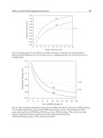
Notice that the expression in equation (10) has the form of a linear relationship with slope k,
and scaling the argument induces a linear shift of the function, and leaves both the form and
slope k unchanged. Plotting to the log scale as shown in Figure 3, we get a long tail showing
a few nodes dominate the transmission power compared to the majority, similar to the Power

Law (S. B. Lowen and M. C. Teich (1970)).
Properties of power laws - Scale invariance: The main property of power laws that makes
them interesting is their scale invariance. Given a relation f
(x) = ax
k
or, any homogeneous
polynomial, scaling the argument x by a constant factor causes only a proportionate scaling
of the function itself. From the equation (10), we can infer that the property is scale invariant
even with clustering c nodes in a given radius k.
f
(cd) = k(cd
2
) = c
k
f (d)α f (d) (10)
This is validated from the simulation results (Vasanth Iyer (G. Rama Murthy)) obtained in Fig-
ure (2), which show optimal results, minimum loading per node (Vasanth Iyer (S.S. Iyengar)),
when clustering is
≤ 20% as expected from the above derivation.
3.2 MAC Layer Routing
The IEEE 802.15.4 (Joseph Polastre (Jason Hill)) is a standard for sensor network MAC inter-
operability, it defines a standard for the radios present at each node to reliably communicate
with each other. As the radios consume lots of power the MAC protocol for best performance
uses Idle, Sleep and Listen modes to conserve battery. The radios are scheduled to periodically
listen to the channel for any activity and receive any packets, otherwise it goes to idle, or sleep
mode. The MAC protocol also needs to take care of collision as the primary means of commu-
nication is using broadcast mode. The standard carrier sense multiple access (CSMA) protocol
is used to share the channel for simultaneous communications. Sensor network variants of
CSMA such as B-MAC and S-MAC Joseph Polastre (Jason Hill) have evolved, which allows to
Sensors S

1
S
2
S
3
S
4
S
5
S
6
S
7
S
8
Value 4.7 ±
2.0
1.6
±
1.6
3.0
±
1.5
1.8
±
1.0
4.7
±
1.0
1.6

±
0.8
3.0
±
0.75
1.8
±
0.5
Group - - - - - - - -
Table 1. A typical random measurements from sensors showing non-linearity in ranges
better handle passive listening, and used low-power listening(LPL). The performance charac-
teristic of MAC based protocols for varying density (small, medium and high) deployed are
shown in Figure 3. As it is seen it uses best effort routing (least cross-layer overhead), and
maintains a constant throughput, the depletion curve for the MAC also follows the Power
Law depletion curve, and has a higher bound when power-aware scheduling such LPL and
Sleep states are further used for idle optimization.
3.2.1 DHT KEY Lookup
Topology of the overlay network uses an addressing which is generated by consistent hashing
of the node-id, so that the addressing is evenly distributed across all nodes. The new data is
stored with its
< KEY > which is also generated the same way as the node address range. If
the specific node is not in the range the next node in the clockwise direction is assigned the
data for that
< KE Y >. From theorem:4, we have that the average number of hops to retrieve
the value for the
< KE Y, VALUE > is only O(lg n) hops. The routing table can be tagged with
application specific items, which are further used by upper layer during query retrieval.
4. Comparison of DCS and Data Aggregation
In Section 4 and 5, we have seen various data processing algorithms, in terms of communi-
cation cost they are comparable. In this Section, we will look into two design factors of the

distributed framework:
1. Assumption1: How well the individual sensor signal sparsity can be represented.
2. Assumption2: What would be the minimum measurement possible by using joint spar-
sity model from equation (5).
3. Assumption3: The maximum possible basis representations for the joint ensemble co-
efficients.
4. Assumption4: A cost function search which allows to represent the best basis without
overlapping coefficients.
5. Assumption5: Result validation using regression analysis, such package R (Owen Jones
(Robert Maillardet)).
The design framework allows to pre-process individual sensor sparse measurement, and uses
a computationally efficient algorithm to perform in-network data fusion.
To use an example data-set, we will use four random measurements obtained by multiple
sensors, this is shown in Table 1. It has two groups of four sensors each, as shown the mean
value are the same for both the groups and the variance due to random sensor measurements
vary with time. The buffer is created according to the design criteria (1), which preserves
the sparsity of the individual sensor readings, this takes three values for each sensor to be
represented as shown in Figure (4).
Distributed Compressed Sensing of Sensor Data 59
LEACH-S
LEACH-E
CRF
DIRECT
0
10
20
30
40
50
60

70
80
90
100
Energy dissipation & loading per node
5% 10% 20% 30% 40% 50%
Percentage of cluster heads
P*
2P*
Fig. 2. Cost function for managing
residual energy using LEACH rout-
ing.
LEACH
SPEED
Diffusion
0
10
20
30
40
50
60
70
80
90
SPARSE
MEDIUM
DENSE
140m 75m440m
2 2

2
Node density
DENSE
DENSE
Power-Law
n=100, Tx range=50m CONST
Interference Losses
Energy Depletion
50m
2
Fig. 3. Power-aware MAC using
multi-hop routing.
Notice that the expression in equation (10) has the form of a linear relationship with slope k,
and scaling the argument induces a linear shift of the function, and leaves both the form and
slope k unchanged. Plotting to the log scale as shown in Figure 3, we get a long tail showing
a few nodes dominate the transmission power compared to the majority, similar to the Power
Law (S. B. Lowen and M. C. Teich (1970)).
Properties of power laws - Scale invariance: The main property of power laws that makes
them interesting is their scale invariance. Given a relation f
(x) = ax
k
or, any homogeneous
polynomial, scaling the argument x by a constant factor causes only a proportionate scaling
of the function itself. From the equation (10), we can infer that the property is scale invariant
even with clustering c nodes in a given radius k.
f
(cd) = k(cd
2
) = c
k

f (d)α f (d) (10)
This is validated from the simulation results (Vasanth Iyer (G. Rama Murthy)) obtained in Fig-
ure (2), which show optimal results, minimum loading per node (Vasanth Iyer (S.S. Iyengar)),
when clustering is
≤ 20% as expected from the above derivation.
3.2 MAC Layer Routing
The IEEE 802.15.4 (Joseph Polastre (Jason Hill)) is a standard for sensor network MAC inter-
operability, it defines a standard for the radios present at each node to reliably communicate
with each other. As the radios consume lots of power the MAC protocol for best performance
uses Idle, Sleep and Listen modes to conserve battery. The radios are scheduled to periodically
listen to the channel for any activity and receive any packets, otherwise it goes to idle, or sleep
mode. The MAC protocol also needs to take care of collision as the primary means of commu-
nication is using broadcast mode. The standard carrier sense multiple access (CSMA) protocol
is used to share the channel for simultaneous communications. Sensor network variants of
CSMA such as B-MAC and S-MAC Joseph Polastre (Jason Hill) have evolved, which allows to
Sensors S
1
S
2
S
3
S
4
S
5
S
6
S
7
S

8
Value 4.7 ±
2.0
1.6 ±
1.6
3.0 ±
1.5
1.8 ±
1.0
4.7 ±
1.0
1.6 ±
0.8
3.0 ±
0.75
1.8 ±
0.5
Group - - - - - - - -
Table 1. A typical random measurements from sensors showing non-linearity in ranges
better handle passive listening, and used low-power listening(LPL). The performance charac-
teristic of MAC based protocols for varying density (small, medium and high) deployed are
shown in Figure 3. As it is seen it uses best effort routing (least cross-layer overhead), and
maintains a constant throughput, the depletion curve for the MAC also follows the Power
Law depletion curve, and has a higher bound when power-aware scheduling such LPL and
Sleep states are further used for idle optimization.
3.2.1 DHT KEY Lookup
Topology of the overlay network uses an addressing which is generated by consistent hashing
of the node-id, so that the addressing is evenly distributed across all nodes. The new data is
stored with its
< KEY > which is also generated the same way as the node address range. If

the specific node is not in the range the next node in the clockwise direction is assigned the
data for that
< KE Y >. From theorem:4, we have that the average number of hops to retrieve
the value for the
< KE Y, VALUE > is only O(lg n) hops. The routing table can be tagged with
application specific items, which are further used by upper layer during query retrieval.
4. Comparison of DCS and Data Aggregation
In Section 4 and 5, we have seen various data processing algorithms, in terms of communi-
cation cost they are comparable. In this Section, we will look into two design factors of the
distributed framework:
1. Assumption1: How well the individual sensor signal sparsity can be represented.
2. Assumption2: What would be the minimum measurement possible by using joint spar-
sity model from equation (5).
3. Assumption3: The maximum possible basis representations for the joint ensemble co-
efficients.
4. Assumption4: A cost function search which allows to represent the best basis without
overlapping coefficients.
5. Assumption5: Result validation using regression analysis, such package R (Owen Jones
(Robert Maillardet)).
The design framework allows to pre-process individual sensor sparse measurement, and uses
a computationally efficient algorithm to perform in-network data fusion.
To use an example data-set, we will use four random measurements obtained by multiple
sensors, this is shown in Table 1. It has two groups of four sensors each, as shown the mean
value are the same for both the groups and the variance due to random sensor measurements
vary with time. The buffer is created according to the design criteria (1), which preserves
the sparsity of the individual sensor readings, this takes three values for each sensor to be
represented as shown in Figure (4).
Sensor Fusion and Its Applications60
0 0 1.6 0 0
3.1

4.7 6.7 2.7 1.6 3.2 0 3.0 4.5 1.5 1.8 2.8 0.8
4.7
2.4
Signal-1
3.0 1.80 0
2.7
0 0 1.6 0 0
3.1
4.7 5.7 3.7 1.6 2.4 0.8 3.0 3.7 2.2 1.8 2.3 1.3
4.7
2.4
Signal-2
3.0 1.80 0
2.7
2.7
M e a s u r e d L e v e l
M e a n
(a) Post-Processing and Data Aggregation
2.1 1.6
3.7
1.8 0 0 0 0 0.5
3.8 1.72.6 1.7 0.07 0 1.17
3.2 0.3 1.4
0 0 00
1
4.7 6.7 2.7 1.6 3.2 0 3.0 4.5 1.5 1.8 2.8 0.8
5.5 1.6 -1
1.6
-0.7 -0.1
0 0 -0.40.57

0.9 0.04 -0.10.04 0.28-0.20.28
1.9 1.3 0.8 0 0.03 0 0.6 0 0 -0.20.28
-1.1 -0.2 -0.4 -0.7 0
0.5 0.9 0.1 -0.3 0.2 -0.2
-0.5 0.9 -0.1 0.2 -0.4
+
Signal-1 + Signal-2
1 0 1 0 0 0 0 0 0 0 0 0 0
12
6
2
3
1
1
0
1
1
0
0 0
0
0
0
0 0 0
S1 S4 S5 S11 S32
Best Basis x > 1: {4.6, 1.6, 2.2. 2.8}
Best Basis and correlated: {3.2 mean, Range = 1.6, 0.75}
Correlated Variance: {Range = 1.6, 0.6}
K
3.2 1.3 1.7 1.6 1 0 0 0 0 0 0 0 0 0 0 0
3.2 0.6 0.8 1.6 1 0 0 0 0 0 0 0 0 0 0 0

1.3 1.7
0.6 0.8
0.6 1.6
-1.6 -0.6
M e a s u r e d L e v e l s
(b) Pre-Processing and Sensor Data Fusion
Fig. 4. Sensor Value Estimation with Aggregation and Sensor Fusion
In the case of post-processing algorithms, which optimizes on the space and the number of
bits needed to represent multi-sensor readings, the fusing sensor calculates the average or the
mean from the values to be aggregated into a single value. From our example data, we see that
for both the data-sets gives the same end result, in this case µ
= 2.7 as shown in the output
plot of Figure 4(a). Using the design criteria (1), which specifies the sparse representation is
not used by post-processing algorithms. Due to this dynamic features are lost during data
aggregation step.
The pre-processing step uses Discrete Wavelet Transform (DWT) (Arne Jensen and Anders
la Cour-Harbo (2001)) on the signal, and may have to recursively apply the decomposition
to arrive at a sparse representation, this pre-process is shown in Figure 4(b). This step uses
the design criteria (1), which specifies the small number of significant coefficients needed to
represent the given signal measured. As seen in Figure 4(b), each level of decomposition
reduces the size of the coefficients. As memory is constrained, we use up to four levels of
decomposition with a possible of 26 different representations, as computed by equation (2).
These uses the design criteria (3) for lossless reconstruction of the original signal.
The next step of pre-processing is to find the best basis, we let a vector Basis of the same
length as cost values representing the basis, this method uses Algorithm 1. The indexing of
the two vector is the same and are enumerated in Figure of 4(b). In Figure 4(b), we have
marked a basis with shaded boxes. This basis is then represented by the vector. The basis
search, which is part of design criteria (4), allows to represent the best coefficients for inter
and intra sensor features. It can be noticed that the values are not averages or means of the
signal representation, it preserves the actual sensor outputs. As an important design criteria

(2), which calibrates the minimum possible sensitivity of the sensor. The output in figure 4(b),
shows the constant estimate of S
3
, S
7
which is Z
C
= 2.7 from equation (4).
Sensors S
1
S
2
S
3
S
4
S
5
S
6
S
7
S
8
i.i.d.
1
2.7 0 1.5 0.8 3.7 0.8 2.25 1.3
i.i.d.
2
4.7 1.6 3 1.8 4.7 1.6 3 1.8

i.i.d.
3
6.7 3.2 4.5 2.8 5.7 2.4 3.75 2.3
Table 2. Sparse representation of sensor values from Table:1
To represent the variance in four sensors, a basis search is performed which finds coefficients
of sensors which matches the same columns. In this example, we find Z
j
= 1.6, 0.75 from
equation (4), which are the innovation component.
Basis
= [0 0 1 0 1 0 0 1 1 0 0 0 0 0 0 0 0 0 0 0 0 0 0 0 0 0 0 0 0 0]
Correlated range = [0 0 0 0 1 0 0 1 0 0 0 0 0 0 0 0 0 0 0 0 0 0 0 0 0 0 0 0 0 0]
4.1 Lower Bound Validation using Covariance
The Figure 4(b) shows lower bound of the overlapped sensor i.i.d. of S
1
− S
8
, as shown it
is seen that the lower bound is unique to the temporal variations of S
2
. In our analysis we
will use a general model which allows to detect sensor faults. The binary model can result
from placing a threshold on the real-valued readings of sensors. Let m
n
be the mean normal
reading and m
f
the mean event reading for a sensor. A reasonable threshold for distinguishing
between the two possibilities would be 0.5
(

m
n
+m
f
2
). If the errors due to sensor faults and the
fluctuations in the environment can be modeled by Gaussian distributions with mean 0 and a
standard deviation σ, the fault probability p would indeed be symmetric. It can be evaluated
using the tail probability of a Gaussian Bhaskar Krishnamachari (Member), the Q-function, as
follows:
p
= Q

(0.5(
m
n
+m
f
2
) − m
n
)

σ
= Q

m
f
−m
n

2σ

(11)
From the measured i.i.d. value sets we need to determine if they have any faulty sensors.
This can be shown from equation (11) that if the correlated sets can be distinguished from the
mean values then it has a low probability of error due to sensor faults, as sensor faults are
not correlated. Using the statistical analysis package R Owen Jones (Robert Maillardet), we
determine the correlated matrix of the sparse sensor outputs as shown This can be written in
a compact matrix form if we observe that for this case the covariance matrix is diagonal, this
is,
Σ
=




ρ
1
0 0
0 ρ
2
0
: :
 :
0 0 ρ
d





(12)
The correlated co-efficient are shown matrix (13) the corresponding diagonal elements are
highlighted. Due to overlapping reading we see the resulting matrix shows that S
1
and S
2
have higher index. The result sets is within the desired bounds of the previous analysis using
DWT. Here we not only prove that the sensor are not faulty but also report a lower bound of
the optimal correlated result sets, that is we use S
2
as it is the lower bound of the overlapping
ranges.
Distributed Compressed Sensing of Sensor Data 61
0 0 1.6 0 0
3.1
4.7 6.7 2.7 1.6 3.2 0 3.0 4.5 1.5 1.8 2.8 0.8
4.7
2.4
Signal-1
3.0 1.80 0
2.7
0 0 1.6 0 0
3.1
4.7 5.7 3.7 1.6 2.4 0.8 3.0 3.7 2.2 1.8 2.3 1.3
4.7
2.4
Signal-2
3.0 1.80 0
2.7
2.7

M e a s u r e d L e v e l
M e a n
(a) Post-Processing and Data Aggregation
2.1 1.6
3.7
1.8 0 0 0 0 0.5
3.8 1.72.6 1.7 0.07 0 1.17
3.2 0.3 1.4
0 0 00
1
4.7 6.7 2.7 1.6 3.2 0 3.0 4.5 1.5 1.8 2.8 0.8
5.5 1.6 -1
1.6
-0.7 -0.1
0 0 -0.40.57
0.9 0.04 -0.10.04 0.28-0.20.28
1.9 1.3 0.8 0 0.03 0 0.6 0 0 -0.20.28
-1.1 -0.2 -0.4 -0.7 0
0.5 0.9 0.1 -0.3 0.2 -0.2
-0.5 0.9 -0.1 0.2 -0.4
+
Signal-1 + Signal-2
1 0 1 0 0 0 0 0 0 0 0 0 0
12
6
2
3
1
1
0

1
1
0
0 0
0
0
0
0 0 0
S1 S4 S5 S11 S32
Best Basis x > 1: {4.6, 1.6, 2.2. 2.8}
Best Basis and correlated: {3.2 mean, Range = 1.6, 0.75}
Correlated Variance: {Range = 1.6, 0.6}
K
3.2 1.3 1.7 1.6 1 0 0 0 0 0 0 0 0 0 0 0
3.2 0.6 0.8 1.6 1 0 0 0 0 0 0 0 0 0 0 0
1.3 1.7
0.6 0.8
0.6 1.6
-1.6 -0.6
M e a s u r e d L e v e l s
(b) Pre-Processing and Sensor Data Fusion
Fig. 4. Sensor Value Estimation with Aggregation and Sensor Fusion
In the case of post-processing algorithms, which optimizes on the space and the number of
bits needed to represent multi-sensor readings, the fusing sensor calculates the average or the
mean from the values to be aggregated into a single value. From our example data, we see that
for both the data-sets gives the same end result, in this case µ
= 2.7 as shown in the output
plot of Figure 4(a). Using the design criteria (1), which specifies the sparse representation is
not used by post-processing algorithms. Due to this dynamic features are lost during data
aggregation step.

The pre-processing step uses Discrete Wavelet Transform (DWT) (Arne Jensen and Anders
la Cour-Harbo (2001)) on the signal, and may have to recursively apply the decomposition
to arrive at a sparse representation, this pre-process is shown in Figure 4(b). This step uses
the design criteria (1), which specifies the small number of significant coefficients needed to
represent the given signal measured. As seen in Figure 4(b), each level of decomposition
reduces the size of the coefficients. As memory is constrained, we use up to four levels of
decomposition with a possible of 26 different representations, as computed by equation (2).
These uses the design criteria (3) for lossless reconstruction of the original signal.
The next step of pre-processing is to find the best basis, we let a vector Basis of the same
length as cost values representing the basis, this method uses Algorithm 1. The indexing of
the two vector is the same and are enumerated in Figure of 4(b). In Figure 4(b), we have
marked a basis with shaded boxes. This basis is then represented by the vector. The basis
search, which is part of design criteria (4), allows to represent the best coefficients for inter
and intra sensor features. It can be noticed that the values are not averages or means of the
signal representation, it preserves the actual sensor outputs. As an important design criteria
(2), which calibrates the minimum possible sensitivity of the sensor. The output in figure 4(b),
shows the constant estimate of S
3
, S
7
which is Z
C
= 2.7 from equation (4).
Sensors S
1
S
2
S
3
S

4
S
5
S
6
S
7
S
8
i.i.d.
1
2.7 0 1.5 0.8 3.7 0.8 2.25 1.3
i.i.d.
2
4.7 1.6 3 1.8 4.7 1.6 3 1.8
i.i.d.
3
6.7 3.2 4.5 2.8 5.7 2.4 3.75 2.3
Table 2. Sparse representation of sensor values from Table:1
To represent the variance in four sensors, a basis search is performed which finds coefficients
of sensors which matches the same columns. In this example, we find Z
j
= 1.6, 0.75 from
equation (4), which are the innovation component.
Basis
= [0 0 1 0 1 0 0 1 1 0 0 0 0 0 0 0 0 0 0 0 0 0 0 0 0 0 0 0 0 0]
Correlated range = [0 0 0 0 1 0 0 1 0 0 0 0 0 0 0 0 0 0 0 0 0 0 0 0 0 0 0 0 0 0]
4.1 Lower Bound Validation using Covariance
The Figure 4(b) shows lower bound of the overlapped sensor i.i.d. of S
1

− S
8
, as shown it
is seen that the lower bound is unique to the temporal variations of S
2
. In our analysis we
will use a general model which allows to detect sensor faults. The binary model can result
from placing a threshold on the real-valued readings of sensors. Let m
n
be the mean normal
reading and m
f
the mean event reading for a sensor. A reasonable threshold for distinguishing
between the two possibilities would be 0.5
(
m
n
+m
f
2
). If the errors due to sensor faults and the
fluctuations in the environment can be modeled by Gaussian distributions with mean 0 and a
standard deviation σ, the fault probability p would indeed be symmetric. It can be evaluated
using the tail probability of a Gaussian Bhaskar Krishnamachari (Member), the Q-function, as
follows:
p
= Q

(0.5(
m

n
+m
f
2
) − m
n
)

σ
= Q

m
f
−m
n
2σ

(11)
From the measured i.i.d. value sets we need to determine if they have any faulty sensors.
This can be shown from equation (11) that if the correlated sets can be distinguished from the
mean values then it has a low probability of error due to sensor faults, as sensor faults are
not correlated. Using the statistical analysis package R Owen Jones (Robert Maillardet), we
determine the correlated matrix of the sparse sensor outputs as shown This can be written in
a compact matrix form if we observe that for this case the covariance matrix is diagonal, this
is,
Σ
=





ρ
1
0 0
0 ρ
2
0
: :
 :
0 0 ρ
d




(12)
The correlated co-efficient are shown matrix (13) the corresponding diagonal elements are
highlighted. Due to overlapping reading we see the resulting matrix shows that S
1
and S
2
have higher index. The result sets is within the desired bounds of the previous analysis using
DWT. Here we not only prove that the sensor are not faulty but also report a lower bound of
the optimal correlated result sets, that is we use S
2
as it is the lower bound of the overlapping
ranges.
Sensor Fusion and Its Applications62
Σ =
















−→
4.0 3.20 3.00 2.00 2.00 1.60 1.5 1.0
3.2
−−→
2.56 2.40 1.60 1.60 1.28 1.20 0.80
3.0 2.40
−−→
2.250 1.50 1.50 1.20 1.125 0.75
2.0 1.60 1.50
−−→
1.00 1.00 0.80 0.75 0.5
2.0 1.60 1.50 1.00
−−→
1.00 0.80 0.75 0.5
1.6 1.28 1.20 0.80 0.80
−−→

0.64 0.60 0.4
1.5 1.20 1.125 0.75 0.75 0.60
−−−→
0.5625 0.375
1.0 0.80 0.750 0.50 0.50 0.40 0.375
−−→
0.250















(13)
5. Conclusion
In this topic, we have discussed a distributed framework for correlated multi-sensor mea-
surements and data-centric routing. The framework, uses compressed sensing to reduce the
number of required measurements. The joint sparsity model, further allows to define the sys-
tem accuracy in terms of the lowest range, which can be measured by a group of sensors. The
sensor fusion algorithms allows to estimate the physical parameter, which is being measured
without any inter sensor communications. The reliability of the pre-processing and sensor

faults are discussed by comparing DWT and Covariance methods.
The complexity model is developed which allows to describe the encoding and decoding of
the data. The model tends to be easy for encoding, and builds more complexity at the joint
decoding level, which are nodes with have more resources as being the decoders.
Post processing and data aggregation are discussed with cross-layer protocols at the network
and the MAC layer, its implication to data-centric routing using DHT is discussed, and com-
pared with the DCS model. Even though these routing algorithms are power-aware, the model
does not scale in terms of accurately estimating the physical parameters at the sensor level,
making sensor driven processing more reliable for such applications.
6. Theoretical Bounds
The computational complexities and its theoretical bounds are derived for categories of sensor
pre-, post processing and routing algorithms.
6.1 Pre-Processing
Theorem 1. The Slepian-Wolf rate as referenced in the region for two arbitrarily correlated sources x
and y is bounded by the following inequalities, this theorem can be adapted using equation
R
x
≥ H

x
y

, R
y
≥ H

y
x

and R

x
+ R
y
≥ H
(
x, y
)
(14)
Theorem 2. minimal spanning tree (MST) computational and time complexity for correlated den-
drogram. First considering the computational complexity let us assume n patterns in d-dimensional
space. To make c clusters using d
min
(D
i
, Dj) a distance measure of similarity. We need once for
all, need to calculate n
(n − 1) interpoint distance table. The space complexity is n
2
, we reduce it to
lg
(n) entries. Finding the minimum distance pair (for the first merging) requires that we step through
the complete list, keeping the index of the smallest distance. Thus, for the first step, the complexity is
O
(n(n −1))(d
2
+ 1) = O(n
2
d
2
). For clusters c the number of steps is n(n −1) −c unused distances.

The full-time complexity is O
(n(n −1) − c) or O(cn
2
d
2
).
Algorithm 1 DWT: Using a cost function for searching the best sparse representation of a
signal.
1: Mark all the elements on the bottom level
2: Let j = J
3: Let k = 0
4: Compare the cost v
1
of the element k on level (j − 1) (counting from the left on that level)
to the sum v
2
of the cost values of the element 2k and the 2k + 1 on the level j.
5: if v
1
≤ v
2
, all marks below element k on level j −1 are deleted, and element k is marked.
6: if v
1
> v
2
, the cost value v
1
of element k is replaced with v
2

k = k + 1. If there are more
elements on level j (if k
< 2
j−1
−1) ), go to step 4.
7: j = j − 1. If j > 1, go to step 3.
8: The marked sparse representation has the lowest possible cost value, having no overlaps.
6.2 Post-processing
Theorem 3. Properties of Pre-fix coding: For any compression algorithm which assigns prefix codes
and to uniquely be decodable. Let us define the kraft Number and is a measure of the size of L. We
see that if L is 1, 2
−L
is .5. We know that we cannot have more than two L’s of .5. If there are more
that two L’s of .5, then K
> 1. Similarly, we know L can be as large as we want. Thus, 2
−L
can be as
small as we want, so K can be as small as we want. Thus we can intuitively see that there must be a
strict upper bound on K, and no lower bound. It turns out that a prefix-code only exists for the codes
IF AND ONLY IF:
K
≤ 1 (15)
The above equation is the Kraft inequality. The success of transmission can be further calculated by
using the equation For a minimum pre-fix code a
= 0.5 as 2
−L
≤ 1 for a unique decodability.
Iteration a
= 0.5
In order to extend this scenario with distributed source coding, we consider the case of separate encoders

for each source, x
n
and y
n
. Each encoder operates without access to the other source.
Iteration a
≥ 0.5 ≤ 1.0
As in the previous case it uses correlated values as a dependency and constructs the code-book. The
compression rate or efficiency is further enhanced by increasing the correlated CDF higher than a
>
0.5. This produces very efficient code-book and the design is independent of any decoder reference
information. Due to this a success threshold is also predictable, if a
= 0.5 and the cost between L = 1.0
and 2.0 the success
= 50% and for a = 0.9 and L = 1.1, the success = 71%.
6.3 Distributed Routing
Theorem 4. The Cayley Graph (S, E) of a group: Vertices corresponding to the underlying set S.
Edges corresponding to the actions of the generators. (Complete) Chord is a Cayley graph for
(Zn, +).
The routing nodes can be distributed using S
= Z mod n (n = 2
m
) very similar to our simulation
results of LEACH (Vasanth Iyer (G. Rama Murthy)). Generators for one-way hashing can use these
fixed length hash 1, 2, 4, , 2
m
−1. Most complete Distributed Hash Table (DHTs) are Cayley graphs.
Data-centric algorithm Complexity: where Z is the original ID and the key is its hash between 0
−2
m

,
ID
+ key are uniformly distributed in the chord (Vasanth Iyer (S. S. Iyengar)).
Distributed Compressed Sensing of Sensor Data 63
Σ =















−→
4.0 3.20 3.00 2.00 2.00 1.60 1.5 1.0
3.2
−−→
2.56 2.40 1.60 1.60 1.28 1.20 0.80
3.0 2.40
−−→
2.250 1.50 1.50 1.20 1.125 0.75
2.0 1.60 1.50
−−→

1.00 1.00 0.80 0.75 0.5
2.0 1.60 1.50 1.00
−−→
1.00 0.80 0.75 0.5
1.6 1.28 1.20 0.80 0.80
−−→
0.64 0.60 0.4
1.5 1.20 1.125 0.75 0.75 0.60
−−−→
0.5625 0.375
1.0 0.80 0.750 0.50 0.50 0.40 0.375
−−→
0.250















(13)
5. Conclusion

In this topic, we have discussed a distributed framework for correlated multi-sensor mea-
surements and data-centric routing. The framework, uses compressed sensing to reduce the
number of required measurements. The joint sparsity model, further allows to define the sys-
tem accuracy in terms of the lowest range, which can be measured by a group of sensors. The
sensor fusion algorithms allows to estimate the physical parameter, which is being measured
without any inter sensor communications. The reliability of the pre-processing and sensor
faults are discussed by comparing DWT and Covariance methods.
The complexity model is developed which allows to describe the encoding and decoding of
the data. The model tends to be easy for encoding, and builds more complexity at the joint
decoding level, which are nodes with have more resources as being the decoders.
Post processing and data aggregation are discussed with cross-layer protocols at the network
and the MAC layer, its implication to data-centric routing using DHT is discussed, and com-
pared with the DCS model. Even though these routing algorithms are power-aware, the model
does not scale in terms of accurately estimating the physical parameters at the sensor level,
making sensor driven processing more reliable for such applications.
6. Theoretical Bounds
The computational complexities and its theoretical bounds are derived for categories of sensor
pre-, post processing and routing algorithms.
6.1 Pre-Processing
Theorem 1. The Slepian-Wolf rate as referenced in the region for two arbitrarily correlated sources x
and y is bounded by the following inequalities, this theorem can be adapted using equation
R
x
≥ H

x
y

, R
y

≥ H

y
x

and R
x
+ R
y
≥ H
(
x, y
)
(14)
Theorem 2. minimal spanning tree (MST) computational and time complexity for correlated den-
drogram. First considering the computational complexity let us assume n patterns in d-dimensional
space. To make c clusters using d
min
(D
i
, Dj) a distance measure of similarity. We need once for
all, need to calculate n
(n − 1) interpoint distance table. The space complexity is n
2
, we reduce it to
lg
(n) entries. Finding the minimum distance pair (for the first merging) requires that we step through
the complete list, keeping the index of the smallest distance. Thus, for the first step, the complexity is
O
(n(n −1))(d

2
+ 1) = O(n
2
d
2
). For clusters c the number of steps is n(n −1) −c unused distances.
The full-time complexity is O
(n(n −1) − c) or O(cn
2
d
2
).
Algorithm 1 DWT: Using a cost function for searching the best sparse representation of a
signal.
1: Mark all the elements on the bottom level
2: Let j = J
3: Let k = 0
4: Compare the cost v
1
of the element k on level (j − 1) (counting from the left on that level)
to the sum v
2
of the cost values of the element 2k and the 2k + 1 on the level j.
5: if v
1
≤ v
2
, all marks below element k on level j −1 are deleted, and element k is marked.
6: if v
1

> v
2
, the cost value v
1
of element k is replaced with v
2
k = k + 1. If there are more
elements on level j (if k
< 2
j−1
−1) ), go to step 4.
7: j = j − 1. If j > 1, go to step 3.
8: The marked sparse representation has the lowest possible cost value, having no overlaps.
6.2 Post-processing
Theorem 3. Properties of Pre-fix coding: For any compression algorithm which assigns prefix codes
and to uniquely be decodable. Let us define the kraft Number and is a measure of the size of L. We
see that if L is 1, 2
−L
is .5. We know that we cannot have more than two L’s of .5. If there are more
that two L’s of .5, then K
> 1. Similarly, we know L can be as large as we want. Thus, 2
−L
can be as
small as we want, so K can be as small as we want. Thus we can intuitively see that there must be a
strict upper bound on K, and no lower bound. It turns out that a prefix-code only exists for the codes
IF AND ONLY IF:
K
≤ 1 (15)
The above equation is the Kraft inequality. The success of transmission can be further calculated by
using the equation For a minimum pre-fix code a

= 0.5 as 2
−L
≤ 1 for a unique decodability.
Iteration a
= 0.5
In order to extend this scenario with distributed source coding, we consider the case of separate encoders
for each source, x
n
and y
n
. Each encoder operates without access to the other source.
Iteration a
≥ 0.5 ≤ 1.0
As in the previous case it uses correlated values as a dependency and constructs the code-book. The
compression rate or efficiency is further enhanced by increasing the correlated CDF higher than a
>
0.5. This produces very efficient code-book and the design is independent of any decoder reference
information. Due to this a success threshold is also predictable, if a
= 0.5 and the cost between L = 1.0
and 2.0 the success
= 50% and for a = 0.9 and L = 1.1, the success = 71%.
6.3 Distributed Routing
Theorem 4. The Cayley Graph (S, E) of a group: Vertices corresponding to the underlying set S.
Edges corresponding to the actions of the generators. (Complete) Chord is a Cayley graph for
(Zn, +).
The routing nodes can be distributed using S
= Z mod n (n = 2
m
) very similar to our simulation
results of LEACH (Vasanth Iyer (G. Rama Murthy)). Generators for one-way hashing can use these

fixed length hash 1, 2, 4, , 2
m
−1. Most complete Distributed Hash Table (DHTs) are Cayley graphs.
Data-centric algorithm Complexity: where Z is the original ID and the key is its hash between 0
−2
m
,
ID
+ key are uniformly distributed in the chord (Vasanth Iyer (S. S. Iyengar)).
Sensor Fusion and Its Applications64
7. References
S. Lowen and M. Teich. (1970). Power-Law Shot Noise, IEEE Trans Inform volume 36, pages
1302-1318, 1970.
Slepian, D. Wolf, J. (1973). Noiseless coding of correlated information sources. Information
Theory, IEEE Transactions on In Information Theory, IEEE Transactions on, Vol. 19,
No. 4. (06 January 2003), pp. 471-480.
Bhaskar Krishnamachari, S.S. Iyengar. (2004). Distributed Bayesian Algorithms for Fault-
Tolerant Event Region Detection in Wireless Sensor Networks, In: IEEE TRANSAC-
TIONS ON COMPUTERS,VOL. 53, NO. 3, MARCH 2004.
Dror Baron, Marco F. Duarte, Michael B. Wakin, Shriram Sarvotham, and Richard G. Baraniuk.
(2005). Distributed Compressive Sensing. In Proc: Pre-print, Rice University, Texas,
USA, 2005.
Vasanth Iyer, G. Rama Murthy, and M.B. Srinivas. (2008). Min Loading Max Reusability Fusion
Classifiers for Sensor Data Model. In Proc: Second international Conference on Sensor
Technologies and Applications, Volume 00 (August 25 - 31, SENSORCOMM 2008).
Vasanth Iyer, S.S. Iyengar, N. Balakrishnan, Vir. Phoha, M.B. Srinivas. (2009). FARMS: Fusion-
able Ambient Renewable MACS, In: SAS-2009,IEEE 9781-4244-2787, 17th-19th Feb,
New Orleans, USA.
Vasanth Iyer, S. S. Iyengar, Rama Murthy, N. Balakrishnan, and V. Phoha. (2009). Distributed
source coding for sensor data model and estimation of cluster head errors using

bayesian and k-near neighborhood classifiers in deployment of dense wireless sensor
networks, In Proc: Third International Conference on Sensor Technologies and Applications
SENSORCOMM, 17-21 June. 2009.
Vasanth Iyer, S.S. Iyengar, G. Rama Murthy, Kannan Srinathan, Vir Phoha, and M.B. Srinivas.
INSPIRE-DB: Intelligent Networks Sensor Processing of Information using Resilient
Encoded-Hash DataBase. In Proc. Fourth International Conference on Sensor Tech-
nologies and Applications, IARIA-SENSORCOMM, July, 18th-25th, 2010, Venice,
Italy (archived in the Computer Science Digital Library).
Vasanth Iyer, S.S. Iyengar, N. Balakrishnan, Vir. Phoha, M.B. Srinivas. (2009). FARMS: Fusion-
able Ambient Renewable MACS, In: SAS-2009,IEEE 9781-4244-2787, 17th-19th Feb,
New Orleans, USA.
GEM: Graph EMbedding for Routing and DataCentric Storage in Sensor Networks Without
Geographic Information. Proceedings of the First ACM Conference on Embedded
Networked Sensor Systems (SenSys). November 5-7, Redwood, CA.
Owen Jones, Robert Maillardet, and Andrew Robinson. Introduction to Scientific Program-
ming and Simulation Using R. Chapman & Hall/CRC, Boca Raton, FL, 2009. ISBN
978-1-4200-6872-6.
Arne Jensen and Anders la Cour-Harbo. Ripples in Mathematics, Springer Verlag 2001. 246
pp. Softcover ISBN 3-540-41662-5.
S. S. Iyengar, Nandan Parameshwaran, Vir V. Phoha, N. Balakrishnan, and Chuka D Okoye,
Fundamentals of Sensor Network Programming: Applications and Technology.
ISBN: 978-0-470-87614-5 Hardcover 350 pages December 2010, Wiley-IEEE Press.
Adaptive Kalman Filter for Navigation Sensor Fusion 65
Adaptive Kalman Filter for Navigation Sensor Fusion
Dah-Jing Jwo, Fong-Chi Chung and Tsu-Pin Weng
X

Adaptive Kalman Filter
for Navigation Sensor Fusion

Dah-Jing Jwo, Fong-Chi Chung
National Taiwan Ocean University, Keelung
Taiwan

Tsu-Pin Weng
EverMore Technology, Inc., Hsinchu
Taiwan

1. Introduction
As a form of optimal estimator characterized by recursive evaluation, the Kalman filter (KF)
(Bar-Shalom, et al, 2001; Brown and Hwang, 1997, Gelb, 1974; Grewal & Andrews, 2001) has
been shown to be the filter that minimizes the variance of the estimation mean square error
(MSE) and has been widely applied to the navigation sensor fusion. Nevertheless, in
Kalman filter designs, the divergence due to modeling errors is critical. Utilization of the KF
requires that all the plant dynamics and noise processes are completely known, and the
noise process is zero mean white noise. If the input data does not reflect the real model, the
KF estimates may not be reliable. The case that theoretical behavior of a filter and its actual
behavior do not agree may lead to divergence problems. For example, if the Kalman filter is
provided with information that the process behaves a certain way, whereas, in fact, it
behaves a different way, the filter will continually intend to fit an incorrect process signal.
Furthermore, when the measurement situation does not provide sufficient information to
estimate all the state variables of the system, in other words, the estimation error covariance
matrix becomes unrealistically small and the filter disregards the measurement.
In various circumstances where there are uncertainties in the system model and noise
description, and the assumptions on the statistics of disturbances are violated since in a
number of practical situations, the availability of a precisely known model is unrealistic due
to the fact that in the modelling step, some phenomena are disregarded and a way to take
them into account is to consider a nominal model affected by uncertainty. The fact that KF
highly depends on predefined system and measurement models forms a major drawback. If
the theoretical behavior of the filter and its actual behavior do not agree, divergence

problems tend to occur. The adaptive algorithm has been one of the approaches to prevent
divergence problem of the Kalman filter when precise knowledge on the models are not
available.
To fulfil the requirement of achieving the filter optimality or to preventing divergence
problem of Kalman filter, the so-called adaptive Kalman filter (AKF) approach (Ding, et al,
4
Sensor Fusion and Its Applications66

2007; El-Mowafy & Mohamed, 2005; Mehra, 1970, 1971, 1972; Mohamed & Schwarz, 1999;
Hide et al., 2003) has been one of the promising strategies for dynamically adjusting the
parameters of the supposedly optimum filter based on the estimates of the unknown
parameters for on-line estimation of motion as well as the signal and noise statistics
available data. Two popular types of the adaptive Kalman filter algorithms include the
innovation-based adaptive estimation (IAE) approach (El-Mowafy & Mohamed, 2005;
Mehra, 1970, 1971, 1972; Mohamed & Schwarz, 1999; Hide et al., 2003) and the adaptive
fading Kalman filter (AFKF) approach (Xia et al., 1994; Yang, et al, 1999, 2004;Yang & Xu,
2003; Zhou & Frank, 1996), which is a type of covariance scaling method, for which
suboptimal fading factors are incorporated. The AFKF incorporates suboptimal fading
factors as a multiplier to enhance the influence of innovation information for improving the
tracking capability in high dynamic maneuvering.
The Global Positioning System (GPS) and inertial navigation systems (INS) (Farrell, 1998;
Salychev, 1998) have complementary operational characteristics and the synergy of both
systems has been widely explored. GPS is capable of providing accurate position
information. Unfortunately, the data is prone to jamming or being lost due to the limitations
of electromagnetic waves, which form the fundamental of their operation. The system is not
able to work properly in the areas due to signal blockage and attenuation that may
deteriorate the overall positioning accuracy. The INS is a self-contained system that
integrates three acceleration components and three angular velocity components with
respect to time and transforms them into the navigation frame to deliver position, velocity
and attitude components. For short time intervals, the integration with respect to time of the

linear acceleration and angular velocity monitored by the INS results in an accurate velocity,
position and attitude. However, the error in position coordinates increase unboundedly as a
function of time. The GPS/INS integration is the adequate solution to provide a navigation
system that has superior performance in comparison with either a GPS or an INS stand-
alone system. The GPS/INS integration is typically carried out through the Kalman filter.
Therefore, the design of GPS/INS integrated navigation system heavily depends on the
design of sensor fusion method. Navigation sensor fusion using the AKF will be discussed.
A hybrid approach will be presented and performance will be evaluated on the loosely-
coupled GPS/INS navigation applications.
This chapter is organized as follows. In Section 2, preliminary background on adaptive
Kalman filters is reviewed. An IAE/AFKF hybrid adaptation approach is introduced in
Section 3. In Section 4, illustrative examples on navigation sensor fusion are given.
Conclusions are given in Section 5.

2. Adaptive Kalman Filters
The process model and measurement model are represented as

kkkk
wxΦx 
1
(1a)

kkkk
vxHz  (1b)
where the state vector
n
k
x , process noise vector
n
k

w , measurement
vector
m
k
z , and measurement noise vector
m
k
v . In Equation (1), both the vectors
k
w and
k
v are zero mean Gaussian white sequences having zero crosscorrelation with
each other:







ki
ki
k
ik
,0
,
][
T
Q
wwE

;






ki
ki
k
ik
,0
,
][
T
R
vvE
;
kandiallfor
ik
0vwE ][
T
(2)
where
k
Q
is the process noise covariance matrix,
k
R
is the measurement noise covariance

matrix,
t
k
e


F
Φ is the state transition matrix, and t

is the sampling interval, ][E
represents expectation, and superscript “T” denotes matrix transpose.
The discrete-time Kalman filter algorithm is summarized as follow:
Prediction steps/time update equations:

kkk
xΦx
ˆˆ
1



(3)

kkkkk
QΦPΦP 


T
1
(4)

Correction steps/measurement update equations:

1TT
][


kkkkkkk
RHPHHPK (5)

]
ˆ
[
ˆˆ


kkkkkk
xHzKxx (6)



kkkk
PHKIP ][ (7)
A limitation in applying Kalman filter to real-world problems is that the a priori statistics of
the stochastic errors in both dynamic process and measurement models are assumed to be
available, which is difficult in practical application due to the fact that the noise statistics
may change with time. As a result, the set of unknown time-varying statistical parameters of
noise, },{
kk
RQ , needs to be simultaneously estimated with the system state and the error
covariance. Two popular types of the adaptive Kalman filter algorithms include the

innovation-based adaptive estimation (IAE) approach (El-Mowafy and Mohamed, 2005;
Mehra, 1970, 1971, 1972; Mohamed and Schwarz, 1999; Hide et al., 2003; Caliskan & Hajiyev,
2000) and the adaptive fading Kalman filter (AFKF) approach (Xia et al., 1994; Zhou & Frank,
1996), which is a type of covariance scaling method, for which suboptimal fading factors are
incorporated.

2.1 The innovation-based adaptive estimation
The innovation sequences have been utilized by the correlation and covariance-matching
techniques to estimate the noise covariances. The basic idea behind the covariance-matching
approach is to make the actual value of the covariance of the residual consistent with its
theoretical value. The implementation of IAE based AKF to navigation designs has been
widely explored (Hide et al, 2003, Mohamed and Schwarz 1999). Equations (3)-(4) are the
time update equations of the algorithm from k to step 1

k , and Equations (5)-(7) are the
measurement update equations. These equations incorporate a measurement value into a
priori estimation to obtain an improved a posteriori estimation. In the above equations,
k
P is
the error covariance matrix defined by
])
ˆ
)(
ˆ
[(
T
kkkk
E xxxx  , in which
k
x

ˆ
is an estimation
of the system state vector
k
x , and the weighting matrix
k
K is generally referred to as the
Kalman gain matrix. The Kalman filter algorithm starts with an initial condition value,

0
ˆ
x

and

0
P . When new measurement
k
z becomes available with the progression of time, the
estimation of states and the corresponding error covariance would follow recursively ad
infinity. Mehra (1970, 1971, 1972) classified the adaptive approaches into four categories:
Bayesian, maximum likelihood, correlation and covariance matching. The innovation
Adaptive Kalman Filter for Navigation Sensor Fusion 67

2007; El-Mowafy & Mohamed, 2005; Mehra, 1970, 1971, 1972; Mohamed & Schwarz, 1999;
Hide et al., 2003) has been one of the promising strategies for dynamically adjusting the
parameters of the supposedly optimum filter based on the estimates of the unknown
parameters for on-line estimation of motion as well as the signal and noise statistics
available data. Two popular types of the adaptive Kalman filter algorithms include the
innovation-based adaptive estimation (IAE) approach (El-Mowafy & Mohamed, 2005;

Mehra, 1970, 1971, 1972; Mohamed & Schwarz, 1999; Hide et al., 2003) and the adaptive
fading Kalman filter (AFKF) approach (Xia et al., 1994; Yang, et al, 1999, 2004;Yang & Xu,
2003; Zhou & Frank, 1996), which is a type of covariance scaling method, for which
suboptimal fading factors are incorporated. The AFKF incorporates suboptimal fading
factors as a multiplier to enhance the influence of innovation information for improving the
tracking capability in high dynamic maneuvering.
The Global Positioning System (GPS) and inertial navigation systems (INS) (Farrell, 1998;
Salychev, 1998) have complementary operational characteristics and the synergy of both
systems has been widely explored. GPS is capable of providing accurate position
information. Unfortunately, the data is prone to jamming or being lost due to the limitations
of electromagnetic waves, which form the fundamental of their operation. The system is not
able to work properly in the areas due to signal blockage and attenuation that may
deteriorate the overall positioning accuracy. The INS is a self-contained system that
integrates three acceleration components and three angular velocity components with
respect to time and transforms them into the navigation frame to deliver position, velocity
and attitude components. For short time intervals, the integration with respect to time of the
linear acceleration and angular velocity monitored by the INS results in an accurate velocity,
position and attitude. However, the error in position coordinates increase unboundedly as a
function of time. The GPS/INS integration is the adequate solution to provide a navigation
system that has superior performance in comparison with either a GPS or an INS stand-
alone system. The GPS/INS integration is typically carried out through the Kalman filter.
Therefore, the design of GPS/INS integrated navigation system heavily depends on the
design of sensor fusion method. Navigation sensor fusion using the AKF will be discussed.
A hybrid approach will be presented and performance will be evaluated on the loosely-
coupled GPS/INS navigation applications.
This chapter is organized as follows. In Section 2, preliminary background on adaptive
Kalman filters is reviewed. An IAE/AFKF hybrid adaptation approach is introduced in
Section 3. In Section 4, illustrative examples on navigation sensor fusion are given.
Conclusions are given in Section 5.

2. Adaptive Kalman Filters
The process model and measurement model are represented as

kkkk
wxΦx


1
(1a)

kkkk
vxHz


(1b)
where the state vector
n
k
x , process noise vector
n
k
w , measurement
vector
m
k
z , and measurement noise vector
m
k
v . In Equation (1), both the vectors
k

w and
k
v are zero mean Gaussian white sequences having zero crosscorrelation with
each other:







ki
ki
k
ik
,0
,
][
T
Q
wwE
;






ki
ki

k
ik
,0
,
][
T
R
vvE
;
kandiallfor
ik
0vwE ][
T
(2)
where
k
Q
is the process noise covariance matrix,
k
R
is the measurement noise covariance
matrix,
t
k
e


F
Φ is the state transition matrix, and t is the sampling interval, ][E
represents expectation, and superscript “T” denotes matrix transpose.

The discrete-time Kalman filter algorithm is summarized as follow:
Prediction steps/time update equations:

kkk
xΦx
ˆˆ
1



(3)

kkkkk
QΦPΦP 


T
1
(4)
Correction steps/measurement update equations:

1TT
][


kkkkkkk
RHPHHPK (5)

]
ˆ

[
ˆˆ


kkkkkk
xHzKxx (6)



kkkk
PHKIP ][ (7)
A limitation in applying Kalman filter to real-world problems is that the a priori statistics of
the stochastic errors in both dynamic process and measurement models are assumed to be
available, which is difficult in practical application due to the fact that the noise statistics
may change with time. As a result, the set of unknown time-varying statistical parameters of
noise, },{
kk
RQ , needs to be simultaneously estimated with the system state and the error
covariance. Two popular types of the adaptive Kalman filter algorithms include the
innovation-based adaptive estimation (IAE) approach (El-Mowafy and Mohamed, 2005;
Mehra, 1970, 1971, 1972; Mohamed and Schwarz, 1999; Hide et al., 2003; Caliskan & Hajiyev,
2000) and the adaptive fading Kalman filter (AFKF) approach (Xia et al., 1994; Zhou & Frank,
1996), which is a type of covariance scaling method, for which suboptimal fading factors are
incorporated.

2.1 The innovation-based adaptive estimation
The innovation sequences have been utilized by the correlation and covariance-matching
techniques to estimate the noise covariances. The basic idea behind the covariance-matching
approach is to make the actual value of the covariance of the residual consistent with its
theoretical value. The implementation of IAE based AKF to navigation designs has been

widely explored (Hide et al, 2003, Mohamed and Schwarz 1999). Equations (3)-(4) are the
time update equations of the algorithm from k to step 1k , and Equations (5)-(7) are the
measurement update equations. These equations incorporate a measurement value into a
priori estimation to obtain an improved a posteriori estimation. In the above equations,
k
P is
the error covariance matrix defined by
])
ˆ
)(
ˆ
[(
T
kkkk
E xxxx  , in which
k
x
ˆ
is an estimation
of the system state vector
k
x , and the weighting matrix
k
K is generally referred to as the
Kalman gain matrix. The Kalman filter algorithm starts with an initial condition value,

0
ˆ
x

and

0
P . When new measurement
k
z becomes available with the progression of time, the
estimation of states and the corresponding error covariance would follow recursively ad
infinity. Mehra (1970, 1971, 1972) classified the adaptive approaches into four categories:
Bayesian, maximum likelihood, correlation and covariance matching. The innovation
Sensor Fusion and Its Applications68

sequences have been utilized by the correlation and covariance-matching techniques to
estimate the noise covariances. The basic idea behind the covariance-matching approach is
to make the actual value of the covariance of the residual consistent with its theoretical
value.
From the incoming measurement
k
z and the optimal prediction

k
x
ˆ
obtained in the
previous step, the innovations sequence is defined as



kkk
zzυ
ˆ

(8)
The innovation reflects the discrepancy between the predicted measurement

kk
xH
ˆ
and the
actual measurement
k
z . It represents the additional information available to the filter as a
consequence of the new observation
k
z . The weighted innovation, )
ˆ
(


kkkk
xHzK , acts as a
correction to the predicted estimate

k
x
ˆ
to form the estimation
k
x
ˆ
. Substituting the
measurement model Equation (1b) into Equation (8) gives

kkkkk
vxxHυ 

)
ˆ
(
(9)
which is a zero-mean Gaussian white noise sequence. An innovation of zero means that the
two are in complete agreement. The mean of the corresponding error of an unbiased
estimator is zero. By taking variances on both sides, we have the theoretical covariance, the
covariance matrix of the innovation sequence is given by

kkkkkk
E
k
RHPHυυC 
 TT
][

(10a)
which can be written as

kk
T
kkk
T
kkkk
k
RHΓQΓΦPΦHC 

T
)(

(10b)
Defining
k

C
ˆ
as the statistical sample variance estimate of
k

C
, matrix
k

C
ˆ
can be
computed through averaging inside a moving estimation window of size
N




k
jj
jj
N
k

0
T
1
ˆ
υυC

(11)
where
N
is the number of samples (usually referred to the window size);
1
0
 Nkj
is the
first sample inside the estimation window. The window size
N is chosen empirically (a good
size for the moving window may vary from 10 to 30) to give some statistical smoothing.
More detailed discussion can be referred to Gelb (1974), Brown & Hwang (1997), and
Grewal & Andrews (2001).
The benefit of the adaptive algorithm is that it keeps the covariance consistent with the real
performance. The innovation sequences have been utilized by the correlation and
covariance-matching techniques to estimate the noise covariances. The basic idea behind the
covariance-matching approach is to make the actual value of the covariance of the residual
consistent with its theoretical value. This leads to an estimate of
k
R :

T
ˆ
ˆ

kkkk
k
HPHCR



(12)
Based on the residual based estimate, the estimate of process noise
k
Q is obtained:

T
1
T
0
1
ˆ
kkkk
k
jj
jjk
N
ΦPΦPxxQ




(13)

where



kkk
xxx
ˆ
. This equation can also be written in terms of the innovation sequence:

T
ˆˆ
kkk
k
KCKQ

 (14)
For more detailed information derivation for these equations, see Mohamed & Schwarz
(1999).

2.2 The adaptive fading Kalman filter
The idea of fading memory is to apply a factor to the predicted covariance matrix to
deliberately increase the variance of the predicted state vector. The main difference between
different fading memory algorithms is on the calculation of the scale factor.

A. Typical adaptive fading Kalman filter
One of the approaches for adaptive processing is on the incorporation of fading factors. Xia
et al. (1994) proposed a concept of adaptive fading Kalman filter (AFKF) and solved the state
estimation problem. In the AFKF, suboptimal fading factors are introduced into the
nonlinear smoother algorithm. The idea of fading Kalman filtering is to apply a factor
matrix to the predicted covariance matrix to deliberately increase the variance of the
predicted state vector. In the so called AFKF algorithm, suboptimal fading factors are
introduced into the algorithm.

The idea of fading Kalman filtering is to apply a factor matrix to the predicted covariance
matrix to deliberately increase the variance of the predicted state vector:

k
T
kkkkk
QΦPΦλP 

1
(15a)
or

)(
1 k
T
kkkkk
QΦPΦλP 


(15b)
where
),,(
21 mk
diag



λ . The main difference between various fading memory
algorithms is on the calculation of scale factor
k

λ . One approach is to assign the scale factors
as constants. When
1

i

( mi ,,2,1 

), the filtering is in a steady state processing while
1
i

, the filtering may tend to be unstable. For the case 1
i

, it deteriorates to the
standard Kalman filter. There are some drawbacks with constant factors, e.g., as the filtering
proceeds, the precision of the filtering will decrease because the effects of old data tend to
become less and less. The ideal way is to use time-varying factors that are determined
according to the dynamic and observation model accuracy.
To increase the tracking capability, the time-varying suboptimal scaling factor is
incorporated, for on-line tuning the covariance of the predicted state, which adjusts the
filter gain, and accordingly the improved version of AFKF is developed. The optimum
fading factor is:









][
][
,1max
k
k
k
tr
tr
M
N

(16)
Some other choices of the factors are also used:








][
1
,1max
1
kkk
tr
n

MN

;








][,1max
1
kkk
tr
n
MN


;







][
][
,1max

k
k
k
tr
tr
M
N


where
][tr is the trace of matrix. The parameters are given by
Adaptive Kalman Filter for Navigation Sensor Fusion 69

sequences have been utilized by the correlation and covariance-matching techniques to
estimate the noise covariances. The basic idea behind the covariance-matching approach is
to make the actual value of the covariance of the residual consistent with its theoretical
value.
From the incoming measurement
k
z and the optimal prediction

k
x
ˆ
obtained in the
previous step, the innovations sequence is defined as



kkk

zzυ
ˆ
(8)
The innovation reflects the discrepancy between the predicted measurement

kk
xH
ˆ
and the
actual measurement
k
z . It represents the additional information available to the filter as a
consequence of the new observation
k
z . The weighted innovation, )
ˆ
(


kkkk
xHzK , acts as a
correction to the predicted estimate

k
x
ˆ
to form the estimation
k
x
ˆ

. Substituting the
measurement model Equation (1b) into Equation (8) gives

kkkkk
vxxHυ 

)
ˆ
(
(9)
which is a zero-mean Gaussian white noise sequence. An innovation of zero means that the
two are in complete agreement. The mean of the corresponding error of an unbiased
estimator is zero. By taking variances on both sides, we have the theoretical covariance, the
covariance matrix of the innovation sequence is given by

kkkkkk
E
k
RHPHυυC 
 TT
][

(10a)
which can be written as

kk
T
kkk
T
kkkk

k
RHΓQΓΦPΦHC 
T
)(

(10b)
Defining
k

C
ˆ
as the statistical sample variance estimate of
k

C
, matrix
k

C
ˆ
can be
computed through averaging inside a moving estimation window of size
N




k
jj
jj

N
k
0
T
1
ˆ
υυC

(11)
where
N
is the number of samples (usually referred to the window size);
1
0


Nkj
is the
first sample inside the estimation window. The window size
N is chosen empirically (a good
size for the moving window may vary from 10 to 30) to give some statistical smoothing.
More detailed discussion can be referred to Gelb (1974), Brown & Hwang (1997), and
Grewal & Andrews (2001).
The benefit of the adaptive algorithm is that it keeps the covariance consistent with the real
performance. The innovation sequences have been utilized by the correlation and
covariance-matching techniques to estimate the noise covariances. The basic idea behind the
covariance-matching approach is to make the actual value of the covariance of the residual
consistent with its theoretical value. This leads to an estimate of
k
R :

T
ˆ
ˆ
kkkk
k
HPHCR



(12)
Based on the residual based estimate, the estimate of process noise
k
Q is obtained:

T
1
T
0
1
ˆ
kkkk
k
jj
jjk
N
ΦPΦPxxQ





(13)

where


kkk
xxx
ˆ
. This equation can also be written in terms of the innovation sequence:

T
ˆˆ
kkk
k
KCKQ

 (14)
For more detailed information derivation for these equations, see Mohamed & Schwarz
(1999).

2.2 The adaptive fading Kalman filter
The idea of fading memory is to apply a factor to the predicted covariance matrix to
deliberately increase the variance of the predicted state vector. The main difference between
different fading memory algorithms is on the calculation of the scale factor.

A. Typical adaptive fading Kalman filter
One of the approaches for adaptive processing is on the incorporation of fading factors. Xia
et al. (1994) proposed a concept of adaptive fading Kalman filter (AFKF) and solved the state
estimation problem. In the AFKF, suboptimal fading factors are introduced into the

nonlinear smoother algorithm. The idea of fading Kalman filtering is to apply a factor
matrix to the predicted covariance matrix to deliberately increase the variance of the
predicted state vector. In the so called AFKF algorithm, suboptimal fading factors are
introduced into the algorithm.
The idea of fading Kalman filtering is to apply a factor matrix to the predicted covariance
matrix to deliberately increase the variance of the predicted state vector:

k
T
kkkkk
QΦPΦλP 

1
(15a)
or

)(
1 k
T
kkkkk
QΦPΦλP 


(15b)
where
),,(
21 mk
diag




λ . The main difference between various fading memory
algorithms is on the calculation of scale factor
k
λ . One approach is to assign the scale factors
as constants. When
1
i

( mi ,,2,1  ), the filtering is in a steady state processing while
1
i

, the filtering may tend to be unstable. For the case 1
i

, it deteriorates to the
standard Kalman filter. There are some drawbacks with constant factors, e.g., as the filtering
proceeds, the precision of the filtering will decrease because the effects of old data tend to
become less and less. The ideal way is to use time-varying factors that are determined
according to the dynamic and observation model accuracy.
To increase the tracking capability, the time-varying suboptimal scaling factor is
incorporated, for on-line tuning the covariance of the predicted state, which adjusts the
filter gain, and accordingly the improved version of AFKF is developed. The optimum
fading factor is:









][
][
,1max
k
k
k
tr
tr
M
N

(16)
Some other choices of the factors are also used:








][
1
,1max
1
kkk
tr

n
MN

;








][,1max
1
kkk
tr
n
MN


;







][
][

,1max
k
k
k
tr
tr
M
N


where
][tr is the trace of matrix. The parameters are given by
Sensor Fusion and Its Applications70


T
k
T
kkkkk
HΦPΦHM  (17)

T
kkkkk
HQHRCN 
0
(18a)
where













1,
1
][
0,
2
00
0
k
k
k
T
kkk
T


υυ
υυ
C
(19)
Equation (18a) can be modified by multiplying an innovation enhancement weighting factor
γ , and adding an additional term:

T
kkkkk
HQHRγCN 
0
(18b)
In the AFKF, the key parameter is the fading factor matrix
k
λ . The factor γ is introduced
for increasing the tracking capability through the increased weighting of covariance matrix
of the innovation. The value of weighting factor
γ
is tuned to improve the smoothness of
state estimation. A larger weighting factor
γ provides stronger tracking capability, which is
usually selected empirically. The fading memory approach tries to estimate a scale factor to
increase the predicted variance components of the state vector. The variance estimation
method directly calculates the variance factor for the dynamic model.
There are some drawbacks with a constant factor, e.g., as the filtering proceeds, the
precision of the filtering will decrease because the effects of old data will become less and
less. The ideal way is to use a variant scale factor that will be determined based on the
dynamic and observation model accuracy.

B. The strong tracking Kalman filter
Zhou & Frank (1996) proposed a concept of strong tracking Kalman filter (STKF) (Zhou &
Frank, 1996; Jwo & Wang, 2007) and solved the state estimation problem of a class of
nonlinear systems with white noise. In the so called STKF algorithm, suboptimal fading
factors are introduced into the nonlinear smoother algorithm. The STKF has several
important merits, including (1) strong robustness against model uncertainties; (2) good real-
time state tracking capability even when a state jump occurs, no matter whether the system

has reached steady state or not. Zhou et al proved that a filter is called the STKF only if the
filter satisfies the orthogonal principle stated as follows:
Orthogonal principle: The sufficient condition for a filter to be called the STKF only if the
time-varying filter gain matrix be selected on-line such that the state estimation mean-
square error is minimized and the innovations remain orthogonal (Zhou & Frank, 1996):
min]
ˆ
][
ˆ
[ 
T
kkkk
E xxxx

0][ 

T
kjk
E υυ , 2,1,0k , 2,1j (20)
Equation (20) is required for ensuring that the innovation sequence will be remained
orthogonal.
The time-varying suboptimal scaling factor is incorporated, for on-line tuning the
covariance of the predicted state, which adjusts the filter gain, and accordingly the STKF is
developed. The suboptimal scaling factor in the time-varying filter gain matrix is given by:







1
,
ki
ki
c



1,
1,


ki
ki
c
c


(21)
where

][
][
k
k
k
tr
tr
c
αM

N
 (22)
and

T
kkkkkk
HQHRγVN 

(23)

T
k
T
kkkkk
HΦPΦHM  (24)














1,

1
][
0,
1
00
k
k
T
kkk
T
k


υυV
υυ
V
(25)
The key parameter in the STKF is the fading factor matrix
k
λ , which is dependent on three
parameters, including (1)
i

; (2) the forgetting factor (

); (3) and the softening factor (

).
These parameters are usually selected empirically.
mi

i
,,2,1,1 



, which are a priori
selected. If from a priori knowledge, we have the knowledge that
x
will have a large
change, then a large
i

should be used so as to improve the tracking capability of the STKF.
On the other hand, if no a priori knowledge about the plant dynamic, it is commonly
select
1
21



m



 . In such case, the STKF based on multiple fading factors
deteriorates to a STKF based on a single fading factor. The range of the forgetting factor is
10 

, for which 0.95 is commonly used. The softening factor


is utilized to improve
the smoothness of state estimation. A larger

(with value no less than 1) leads to better
estimation accuracy; while a smaller

provides stronger tracking capability. The value is
usually determined empirically through computer simulation and
5.4


is a commonly
selected value.

C. The algorithm proposed by Yang, et al.
An adaptive factor depending on the discrepancy between predicted state from the dynamic
model and the geometric estimated state by using measurements was proposed by Yang et
al (1999, 2003, 2004), where they introduced an adaptive factor

incorporated into for
regulating the error covariance


/)(
T
1
kkkkk
QΦPΦP 



(26)
where

is the single factor given by
























1
10

2
01
1
0
0
~
0
~
~
~
~
1
c
cc
cc
c
c
c
k
k
k
k
k
υ
υ
υ
υ
υ

(27)

It is seen that Equation (15a) with

/1
k
results in Equation (26). In Equation (27), 1
0
c
and
3
1
c are commonly selected values, and
Adaptive Kalman Filter for Navigation Sensor Fusion 71


T
k
T
kkkkk
HΦPΦHM  (17)

T
kkkkk
HQHRCN 
0
(18a)
where













1,
1
][
0,
2
00
0
k
k
k
T
kkk
T


υυ
υυ
C
(19)
Equation (18a) can be modified by multiplying an innovation enhancement weighting factor
γ , and adding an additional term:

T
kkkkk
HQHRγCN 
0
(18b)
In the AFKF, the key parameter is the fading factor matrix
k
λ . The factor γ is introduced
for increasing the tracking capability through the increased weighting of covariance matrix
of the innovation. The value of weighting factor
γ
is tuned to improve the smoothness of
state estimation. A larger weighting factor
γ provides stronger tracking capability, which is
usually selected empirically. The fading memory approach tries to estimate a scale factor to
increase the predicted variance components of the state vector. The variance estimation
method directly calculates the variance factor for the dynamic model.
There are some drawbacks with a constant factor, e.g., as the filtering proceeds, the
precision of the filtering will decrease because the effects of old data will become less and
less. The ideal way is to use a variant scale factor that will be determined based on the
dynamic and observation model accuracy.

B. The strong tracking Kalman filter
Zhou & Frank (1996) proposed a concept of strong tracking Kalman filter (STKF) (Zhou &
Frank, 1996; Jwo & Wang, 2007) and solved the state estimation problem of a class of
nonlinear systems with white noise. In the so called STKF algorithm, suboptimal fading
factors are introduced into the nonlinear smoother algorithm. The STKF has several
important merits, including (1) strong robustness against model uncertainties; (2) good real-
time state tracking capability even when a state jump occurs, no matter whether the system
has reached steady state or not. Zhou et al proved that a filter is called the STKF only if the

filter satisfies the orthogonal principle stated as follows:
Orthogonal principle: The sufficient condition for a filter to be called the STKF only if the
time-varying filter gain matrix be selected on-line such that the state estimation mean-
square error is minimized and the innovations remain orthogonal (Zhou & Frank, 1996):
min]
ˆ
][
ˆ
[ 
T
kkkk
E xxxx

0][ 

T
kjk
E υυ , 2,1,0

k , 2,1

j (20)
Equation (20) is required for ensuring that the innovation sequence will be remained
orthogonal.
The time-varying suboptimal scaling factor is incorporated, for on-line tuning the
covariance of the predicted state, which adjusts the filter gain, and accordingly the STKF is
developed. The suboptimal scaling factor in the time-varying filter gain matrix is given by:







1
,
ki
ki
c



1,
1,


ki
ki
c
c


(21)
where

][
][
k
k
k
tr

tr
c
αM
N
 (22)
and

T
kkkkkk
HQHRγVN 

(23)

T
k
T
kkkkk
HΦPΦHM  (24)















1,
1
][
0,
1
00
k
k
T
kkk
T
k


υυV
υυ
V
(25)
The key parameter in the STKF is the fading factor matrix
k
λ , which is dependent on three
parameters, including (1)
i

; (2) the forgetting factor (

); (3) and the softening factor (


).
These parameters are usually selected empirically.
mi
i
,,2,1,1 

, which are a priori
selected. If from a priori knowledge, we have the knowledge that
x
will have a large
change, then a large
i

should be used so as to improve the tracking capability of the STKF.
On the other hand, if no a priori knowledge about the plant dynamic, it is commonly
select
1
21

m



 . In such case, the STKF based on multiple fading factors
deteriorates to a STKF based on a single fading factor. The range of the forgetting factor is
10 

, for which 0.95 is commonly used. The softening factor

is utilized to improve

the smoothness of state estimation. A larger

(with value no less than 1) leads to better
estimation accuracy; while a smaller

provides stronger tracking capability. The value is
usually determined empirically through computer simulation and
5.4

is a commonly
selected value.

C. The algorithm proposed by Yang, et al.
An adaptive factor depending on the discrepancy between predicted state from the dynamic
model and the geometric estimated state by using measurements was proposed by Yang et
al (1999, 2003, 2004), where they introduced an adaptive factor

incorporated into for
regulating the error covariance


/)(
T
1
kkkkk
QΦPΦP 


(26)
where


is the single factor given by
























1
10
2
01

1
0
0
~
0
~
~
~
~
1
c
cc
cc
c
c
c
k
k
k
k
k
υ
υ
υ
υ
υ

(27)
It is seen that Equation (15a) with


/1
k
results in Equation (26). In Equation (27), 1
0
c
and
3
1
c are commonly selected values, and
Sensor Fusion and Its Applications72


k
k
k

C
υ
υ 
~
(28)
To avoid 0

, it is common to choose










c
c
c
k
k
k
υ
υ
υ
~
~
~
1

(29)
The a priori selected value

is usually selected empirically. If from a priori knowledge, we
have the knowledge that
x
will have a large change, then a small

should be used so as to
improve the tracking capability. The range of the factor is 10 

. The factor is utilized to
improve the smoothness of state estimation. A larger


( 1 ) leads to better estimation
accuracy; while a smaller

provides stronger tracking capability. The value is usually
determined empirically through personal experience or computer simulation using a
heuristic searching scheme. In the case that 1

, it deteriorates to a standard Kalman filter.
In Equation (29), the threshold 5.0c is an average value commonly used. To increase the
tracking capability, the time-varying suboptimal scaling factor need to be properly
designed, for on-line tuning the covariance of the predicted state, which adjusts the filter
gain, and accordingly the improved version of AFKF is able to provide better estimation
accuracy.

2.3 The tuning logic for parameter adaptation
Another type of adaptation can be conducted by introducing a scaling factor directly to the
k
Q
and/or
k
R
matrices. To account for the greater uncertainty, the covariances need to be
updated, through one of the following ways (Bakhache & Nikiforov, 2000; Jwo & Cho, 2007;
Sasiadek, et al, 2000):
(1)
kkk
QQQ 
1
;

kkk
RRR 
1

(2)
)1( 

k
kk

QQ ;
)1( 

k
kk

RR , 1

; 1


(3)
kk
QQ

 ;
kk
RR



For example, if (3) is utilized as an example, the filter equations can be augmented in the
following way:

kkkkk
QΦPΦP




T
1
(30)
1TT
][


kkkkkkk
RHPHHPK


In case that 1


, it deteriorates to the standard Kalman filter.
To detect the discrepancy between
k

C
ˆ
and

k

C , we define the degree of mismatch (DOM)

kk

CC
ˆ
DOM  (31)
Kalman filtering with motion detection is important in target tracking applications. The
innovation information at the present epoch can be employed for timely reflect the change
in vehicle dynamic. Selecting the degree of divergence (DOD) as the trace of innovation
covariance matrix at present epoch (i.e., the window size is one), we have:

)(
TT
kkkk
tr υυυυ 

(32)

This parameter can be utilized for detection of divergence/outliers or adaptation for
adaptive filtering. If the discrepancy for the trace of innovation covariance matrix between
the present (actual) and theoretical value is used, the DOD parameter can be of the form:

)(
T
k
tr
kk



Cυυ 
(33)
The other DOD parameter commonly use as a simple test statistic for an occurrence of
failure detection is based on the normalized innovation squared, defined as the ratio given
by:

kk
kk
k
k
tr
υCυ
C
υυ
1T
T
)(





(34)
For each of the approaches, only one scalar value needs to be determined, and therefore the
fuzzy rules can be simplified resulting in the decrease of computational efficiency.
The logic of adaptation algorithm using covariance-matching technique is described as
follows. When the actual covariance value
k


C
ˆ
is observed, if its value is within the range
predicted by theory
k

C and the difference is very near to zero, this indicates that both
covariances match almost perfectly. If the actual covariance is greater than its theoretical
value, the value of the process noise should be decreased; if the actual covariance is less than
its theoretical value, the value of the process noise should be increased. The fuzzy logic
(Abdelnour,et al , 1993; Jwo & Chang, 2007; Loebis, et al, 2007; Mostov & Soloviev, 1996;
Sasiadek, et al, 2000) is popular mainly due to its simplicity even though some other
approaches such as neural network and genetic algorithm may also be applicable. When the
fuzzy logic approach based on rules of the kind:
IF
〈antecedent〉THEN〈consequent〉
the following rules can be utilized to implement the idea of covariance matching:
A.
k

C
ˆ
is employed
(1) IF
〈 0
ˆ

k


C 〉THEN〈
k
Q is unchanged〉 (This indicates that
k

C
ˆ
is near to zero, the
process noise statistic should be remained.)
(2) IF
〈
0
ˆ

k

C
〉THEN〈
k
Q is increased〉 (This indicates that
k

C
ˆ
is larger than zero,
the process noise statistic is too small and should be increased.)
(3) IF
〈 0
ˆ


k

C 〉THEN〈
k
Q
is decreased〉 (This indicates that
k

C
ˆ
is less than zero, the
process noise statistic is too large and should be decreased.)
B.
DOM is employed
(1) IF
〈 0DOM  〉THEN〈
k
Q is unchanged〉 (This indicates that
k

C
ˆ
is about the same
as
k

C , the process noise statistic should be remained.)
(2) IF
〈 0DOM  〉THEN〈
k

Q is decreased〉 (This indicates that
k

C
ˆ
is less than
k

C , the
process noise statistic should be decreased.)
(3) IF
〈 0DOM  〉THEN〈
k
Q is increased〉 (This indicates that
k

C
ˆ
is larger than
k

C ,
the process noise statistic should be increased.)
C. DOD (

) is employed
Adaptive Kalman Filter for Navigation Sensor Fusion 73


k

k
k

C
υ
υ 
~
(28)
To avoid 0

, it is common to choose









c
c
c
k
k
k
υ
υ
υ
~

~
~
1

(29)
The a priori selected value

is usually selected empirically. If from a priori knowledge, we
have the knowledge that
x
will have a large change, then a small

should be used so as to
improve the tracking capability. The range of the factor is 10



. The factor is utilized to
improve the smoothness of state estimation. A larger

( 1 ) leads to better estimation
accuracy; while a smaller

provides stronger tracking capability. The value is usually
determined empirically through personal experience or computer simulation using a
heuristic searching scheme. In the case that 1


, it deteriorates to a standard Kalman filter.
In Equation (29), the threshold 5.0


c is an average value commonly used. To increase the
tracking capability, the time-varying suboptimal scaling factor need to be properly
designed, for on-line tuning the covariance of the predicted state, which adjusts the filter
gain, and accordingly the improved version of AFKF is able to provide better estimation
accuracy.

2.3 The tuning logic for parameter adaptation
Another type of adaptation can be conducted by introducing a scaling factor directly to the
k
Q
and/or
k
R
matrices. To account for the greater uncertainty, the covariances need to be
updated, through one of the following ways (Bakhache & Nikiforov, 2000; Jwo & Cho, 2007;
Sasiadek, et al, 2000):
(1)
kkk
QQQ 
1
;
kkk
RRR 
1

(2)
)1( 

k

kk

QQ ;
)1( 

k
kk

RR , 1

; 1


(3)
kk
QQ

 ;
kk
RR


For example, if (3) is utilized as an example, the filter equations can be augmented in the
following way:

kkkkk
QΦPΦP





T
1
(30)
1TT
][


kkkkkkk
RHPHHPK


In case that 1




, it deteriorates to the standard Kalman filter.
To detect the discrepancy between
k

C
ˆ
and
k

C , we define the degree of mismatch (DOM)

kk


CC
ˆ
DOM  (31)
Kalman filtering with motion detection is important in target tracking applications. The
innovation information at the present epoch can be employed for timely reflect the change
in vehicle dynamic. Selecting the degree of divergence (DOD) as the trace of innovation
covariance matrix at present epoch (i.e., the window size is one), we have:

)(
TT
kkkk
tr υυυυ 

(32)

This parameter can be utilized for detection of divergence/outliers or adaptation for
adaptive filtering. If the discrepancy for the trace of innovation covariance matrix between
the present (actual) and theoretical value is used, the DOD parameter can be of the form:

)(
T
k
tr
kk


Cυυ 
(33)
The other DOD parameter commonly use as a simple test statistic for an occurrence of
failure detection is based on the normalized innovation squared, defined as the ratio given

by:

kk
kk
k
k
tr
υCυ
C
υυ
1T
T
)(





(34)
For each of the approaches, only one scalar value needs to be determined, and therefore the
fuzzy rules can be simplified resulting in the decrease of computational efficiency.
The logic of adaptation algorithm using covariance-matching technique is described as
follows. When the actual covariance value
k

C
ˆ
is observed, if its value is within the range
predicted by theory
k


C and the difference is very near to zero, this indicates that both
covariances match almost perfectly. If the actual covariance is greater than its theoretical
value, the value of the process noise should be decreased; if the actual covariance is less than
its theoretical value, the value of the process noise should be increased. The fuzzy logic
(Abdelnour,et al , 1993; Jwo & Chang, 2007; Loebis, et al, 2007; Mostov & Soloviev, 1996;
Sasiadek, et al, 2000) is popular mainly due to its simplicity even though some other
approaches such as neural network and genetic algorithm may also be applicable. When the
fuzzy logic approach based on rules of the kind:
IF
〈antecedent〉THEN〈consequent〉
the following rules can be utilized to implement the idea of covariance matching:
A.
k

C
ˆ
is employed
(1) IF
〈 0
ˆ

k

C 〉THEN〈
k
Q is unchanged〉 (This indicates that
k

C

ˆ
is near to zero, the
process noise statistic should be remained.)
(2) IF
〈
0
ˆ

k

C
〉THEN〈
k
Q is increased〉 (This indicates that
k

C
ˆ
is larger than zero,
the process noise statistic is too small and should be increased.)
(3) IF
〈 0
ˆ

k

C 〉THEN〈
k
Q
is decreased〉 (This indicates that

k

C
ˆ
is less than zero, the
process noise statistic is too large and should be decreased.)
B.
DOM is employed
(1) IF
〈 0DOM  〉THEN〈
k
Q is unchanged〉 (This indicates that
k

C
ˆ
is about the same
as
k

C , the process noise statistic should be remained.)
(2) IF
〈 0DOM  〉THEN〈
k
Q is decreased〉 (This indicates that
k

C
ˆ
is less than

k

C , the
process noise statistic should be decreased.)
(3) IF
〈 0DOM  〉THEN〈
k
Q is increased〉 (This indicates that
k

C
ˆ
is larger than
k

C ,
the process noise statistic should be increased.)
C. DOD (

) is employed
Sensor Fusion and Its Applications74

Suppose that

is employed as the test statistic, and
T

represents the chosen threshold.
The following fuzzy rules can be utilized:
(1) IF

〈
T


 〉THEN〈
k
Q is increased〉 (There is a failure or maneuvering reported; the
process noise statistic is too small and needs to be increased)
(2) IF
〈
T


 〉THEN〈
k
Q is decreased〉 (There is no failure or non maneuvering; the
process noise statistic is too large and needs to be decreased)

3. An IAE/AFKF Hybrid Approach
In this section, a hybrid approach (Jwo & Weng, 2008) involving the concept of the two
methods is presented. The proposed method is a hybrid version of the IAE and AFKF
approaches. The ratio of the actual innovation covariance based on the sampled sequence to
the theoretical innovation covariance will be employed for dynamically tuning two filter
parameters - fading factors and measurement noise scaling factors. The method has the
merits of good computational efficiency and numerical stability. The matrices in the KF loop
are able to remain positive definitive.
The conventional KF approach is coupled with the adaptive tuning system (ATS) for
providing two system parameters: fading factor and noise covariance scaling factor. In the
ATS mechanism, both adaptations on process noise covariance (also referred to P-
adaptation herein) and on measurement noise covariance (also referred to R-adaptation

herein) are involved. The idea is based on the concept that when the filter achieves
estimation optimality, the actual innovation covariance based on the sampled sequence and
the theoretical innovation covariance should be equal. In other words, the ratio between the
two should equal one.
(1) Adaptation on process noise covariance.
To account for the uncertainty, the covariance matrix needs to be updated, through
the following way. The new

k
P
can be obtained by multiplying

k
P
by the factor
P
λ
:



kPk
PλP (35)
and the corresponding Kalman gain is given by

1TT
][


kkkkkkk

RHPHHPK (36a)
If representing the new variable
kRk
RλR  , we have

1TT
][


kRkkkkkk
RλHPHHPK (36b)
From Equation (36b), it can be seen that the change of covariance is essentially governed by
two of the parameters:

k
P and
k
R . In addition, the covariance matrix at the measurement
update stage, from Equation (7), can be written as



kkkk
PHKIP ][ (37a)
and



kkkPk
PHKIλP ][ (37b)

Furthermore, based on the relationship given by Equation (35), the covariance matrix at the
prediction stage (i.e., Equation (4)) is given by

kkkkk
QΦPΦP 


T
1
(38)

or, alternatively

kkkkPk
QΦPΦλP 


T
1
(39a)
On the other hand, the covariance matrix can also be approximated by

)(
11 k
T
kkkPkPk
QΦPΦλPλP 





(39b)
where
),,(
21 mP
diag



λ . The main difference between different adaptive fading
algorithms is on the calculation of scale factor
P
λ . One approach is to assign the scale
factors as constants. When
1

i

(
mi ,,2,1 

), the filtering is in a steady state processing
while
1
i

, the filtering may tend to be unstable. For the case
1
i


, it deteriorates to the
standard Kalman filter. There are some drawbacks with constant factors, e.g., as the filtering
proceeds, the precision of the filtering will decrease because the effects of old data tend to
become less and less. The ideal way is to use time varying factors that are determined
according to the dynamic and observation model accuracy.
When there is deviation due to the changes of covariance and measurement noise, the
corresponding innovation covariance matrix can be rewritten as:
kkkk
k
RHPHC 
 T


and

kR
k
kkP
k
RλHPHλC 
 T

(40)
To enhance the tracking capability, the time-varying suboptimal scaling factor is
incorporated, for on-line tuning the covariance of the predicted state, which adjusts the filter
gain, and accordingly the improved version of AFKF is obtained. The
optimum fading
factors can be calculated through the single factor:













)(
)
ˆ
(
,1max)(
k
k
tr
tr
iiPi



C
C
λ
, mi ,2,1 

(41)
where

][tr
is the trace of matrix; 1
i

, is a scaling factor. Increasing
i

will improve
tracking performance.
(2) Adaptation on measurement noise covariance. As the strength of measurement noise changes
with the environment, incorporation of the fading factor only is not able to restrain the
expected estimation accuracy. For resolving these problems, the ATS needs a mechanism for
R-adaptation in addition to P-adaptation, to adjust the noise strengths and improve the filter
estimation performance.
A parameter which represents the ratio of the actual innovation covariance based on the
sampled sequence to the theoretical innovation covariance matrices can be defined as one of
the following methods:
(a) Single factor

)(
)
ˆ
(
)(
k
k
tr
tr
jjRj




C
C
λ 
, nj ,2,1 

(42a)
(b) Multiple factors

jj
jj
j
k
k
)(
)
ˆ
(



C
C

,
nj ,2,1 

(42b)
Adaptive Kalman Filter for Navigation Sensor Fusion 75

Suppose that

is employed as the test statistic, and
T

represents the chosen threshold.
The following fuzzy rules can be utilized:
(1) IF
〈
T


 〉THEN〈
k
Q is increased〉 (There is a failure or maneuvering reported; the
process noise statistic is too small and needs to be increased)
(2) IF
〈
T


 〉THEN〈
k
Q is decreased〉 (There is no failure or non maneuvering; the
process noise statistic is too large and needs to be decreased)

3. An IAE/AFKF Hybrid Approach
In this section, a hybrid approach (Jwo & Weng, 2008) involving the concept of the two
methods is presented. The proposed method is a hybrid version of the IAE and AFKF

approaches. The ratio of the actual innovation covariance based on the sampled sequence to
the theoretical innovation covariance will be employed for dynamically tuning two filter
parameters - fading factors and measurement noise scaling factors. The method has the
merits of good computational efficiency and numerical stability. The matrices in the KF loop
are able to remain positive definitive.
The conventional KF approach is coupled with the adaptive tuning system (ATS) for
providing two system parameters: fading factor and noise covariance scaling factor. In the
ATS mechanism, both adaptations on process noise covariance (also referred to P-
adaptation herein) and on measurement noise covariance (also referred to R-adaptation
herein) are involved. The idea is based on the concept that when the filter achieves
estimation optimality, the actual innovation covariance based on the sampled sequence and
the theoretical innovation covariance should be equal. In other words, the ratio between the
two should equal one.
(1) Adaptation on process noise covariance.
To account for the uncertainty, the covariance matrix needs to be updated, through
the following way. The new

k
P
can be obtained by multiplying

k
P
by the factor
P
λ
:




kPk
PλP (35)
and the corresponding Kalman gain is given by

1TT
][


kkkkkkk
RHPHHPK (36a)
If representing the new variable
kRk
RλR  , we have

1TT
][


kRkkkkkk
RλHPHHPK (36b)
From Equation (36b), it can be seen that the change of covariance is essentially governed by
two of the parameters:

k
P and
k
R . In addition, the covariance matrix at the measurement
update stage, from Equation (7), can be written as




kkkk
PHKIP ][ (37a)
and



kkkPk
PHKIλP ][ (37b)
Furthermore, based on the relationship given by Equation (35), the covariance matrix at the
prediction stage (i.e., Equation (4)) is given by

kkkkk
QΦPΦP 


T
1
(38)

or, alternatively

kkkkPk
QΦPΦλP 


T
1
(39a)
On the other hand, the covariance matrix can also be approximated by

)(
11 k
T
kkkPkPk
QΦPΦλPλP 




(39b)
where
),,(
21 mP
diag



λ . The main difference between different adaptive fading
algorithms is on the calculation of scale factor
P
λ . One approach is to assign the scale
factors as constants. When
1
i

(
mi ,,2,1 
), the filtering is in a steady state processing
while

1
i

, the filtering may tend to be unstable. For the case
1
i

, it deteriorates to the
standard Kalman filter. There are some drawbacks with constant factors, e.g., as the filtering
proceeds, the precision of the filtering will decrease because the effects of old data tend to
become less and less. The ideal way is to use time varying factors that are determined
according to the dynamic and observation model accuracy.
When there is deviation due to the changes of covariance and measurement noise, the
corresponding innovation covariance matrix can be rewritten as:
kkkk
k
RHPHC 
 T


and

kR
k
kkP
k
RλHPHλC 
 T

(40)

To enhance the tracking capability, the time-varying suboptimal scaling factor is
incorporated, for on-line tuning the covariance of the predicted state, which adjusts the filter
gain, and accordingly the improved version of AFKF is obtained. The
optimum fading
factors can be calculated through the single factor:












)(
)
ˆ
(
,1max)(
k
k
tr
tr
iiPi




C
C
λ
, mi ,2,1  (41)
where
][tr
is the trace of matrix; 1
i

, is a scaling factor. Increasing
i

will improve
tracking performance.
(2) Adaptation on measurement noise covariance. As the strength of measurement noise changes
with the environment, incorporation of the fading factor only is not able to restrain the
expected estimation accuracy. For resolving these problems, the ATS needs a mechanism for
R-adaptation in addition to P-adaptation, to adjust the noise strengths and improve the filter
estimation performance.
A parameter which represents the ratio of the actual innovation covariance based on the
sampled sequence to the theoretical innovation covariance matrices can be defined as one of
the following methods:
(a) Single factor

)(
)
ˆ
(
)(
k

k
tr
tr
jjRj



C
C
λ 
, nj ,2,1  (42a)
(b) Multiple factors

jj
jj
j
k
k
)(
)
ˆ
(



C
C

,
nj ,2,1 

(42b)
Sensor Fusion and Its Applications76

It should be noted that from Equation (40) that increasing
k
R
will lead to increasing
k

C ,
and vice versa. This means that time-varying
k
R leads to time-varying
k

C . The value of
R
λ is introduced in order to reduce the discrepancies between
k

C and
k
R . The
adaptation can be implemented through the simple relation:

kRk
RλR  (43)
Further detail regarding the adaptive tuning loop is illustrated by the flow charts shown in
Figs. 1 and 2, where two architectures are presented. Fig. 1 shows the system architecture #1
and Fig. 2 shows the system architecture #2, respectively. In Fig. 1, the flow chart contains

two portions, for which the block indicated by the dot lines is the adaptive tuning system
(ATS) for tuning the values of both P and R parameters; in Fig. 2, the flow chart contains
three portions, for which the two blocks indicated by the dot lines represent the R-
adaptation loop and P-adaptation loop, respectively.

kRk
RλR 

0
ˆ
x
and

0
P



kkk
zzυ
ˆ
kkk
xΦx
ˆˆ
1




)(

1 k
T
kkkPk
QΦPΦλP 


1TT
][


kkkkkkk
RHPHHPK
]
ˆ
[
ˆˆ


kkkkk
zzKxx




kkkk
PHKIP


iiPiiP
)(1max)( λ,λ 




k
jj
jj
N
k
0
T
1
ˆ
υυC


kkkk
k
RHPHC 
 T

)(
)
ˆ
(
)(
k
k
tr
tr
jjR



C
C
λ 
)(
)
ˆ
(
)(
k
k
tr
tr
iiP


C
C
λ 
(Adaptive Tuning System)
R-adaptation
P-adaptation

Fig. 1. Flow chart of the IAE/AFKF hybrid AKF method - system architecture #1

An important remark needs to be pointed out. When the system architecture #1 is employed,
only one window size is needed. It can be seen that the measurement noise covariance of the
innovation covariance matrix hasn’t been updated when performing the fading factor
calculation. In the system architecture #2, the latest information of the measurement noise

strength has already been available when performing the fading factor calculation. However,
one should notice that utilization of the ‘old’ (i.e., before R-adaptation) information is
required. Otherwise, unreliable result may occur since the deviation of the innovation
covariance matrix due to the measurement noise cannot be correctly detected. One strategy
for avoiding this problem can be done by using two different window sizes, one for R-
adaptation loop and the other for P-adaptation loop.

kRk
RλR


0
ˆ
x
and

0
P



kkk
zzυ
ˆ
kkk
xΦx
ˆˆ
1





)(
1 k
T
kkkPk
QΦPΦλP 


1TT
][


kkkkkkk
RHPHHPK
]
ˆ
[
ˆˆ


kkkkk
zzKxx




kkkk
PHKIP




k
jj
jj
P
N
k
0
T
1
ˆ
υυC



iiPiiP
)(1max)( λ,λ




k
jj
jj
R
N
k
0
T

1
ˆ
υυC

kkkk
k
RHPHC 
 T

)(
)
ˆ
(
)(
k
k
tr
tr
jjR


C
C
λ 
)(
)
ˆ
(
)(
k

k
tr
tr
iiP


C
C
λ 
kkkk
k
RHPHC 
 T

R-adaptation loop
P-adaptation loop

Fig. 2. Flow chart of the IAE/AFKF hybrid AKF method - system architecture #2

Adaptive Kalman Filter for Navigation Sensor Fusion 77

It should be noted that from Equation (40) that increasing
k
R
will lead to increasing
k

C ,
and vice versa. This means that time-varying
k

R leads to time-varying
k

C . The value of
R
λ is introduced in order to reduce the discrepancies between
k

C and
k
R . The
adaptation can be implemented through the simple relation:

kRk
RλR  (43)
Further detail regarding the adaptive tuning loop is illustrated by the flow charts shown in
Figs. 1 and 2, where two architectures are presented. Fig. 1 shows the system architecture #1
and Fig. 2 shows the system architecture #2, respectively. In Fig. 1, the flow chart contains
two portions, for which the block indicated by the dot lines is the adaptive tuning system
(ATS) for tuning the values of both P and R parameters; in Fig. 2, the flow chart contains
three portions, for which the two blocks indicated by the dot lines represent the R-
adaptation loop and P-adaptation loop, respectively.

kRk
RλR


0
ˆ
x

and

0
P



kkk
zzυ
ˆ
kkk
xΦx
ˆˆ
1




)(
1 k
T
kkkPk
QΦPΦλP 


1TT
][


kkkkkkk

RHPHHPK
]
ˆ
[
ˆˆ


kkkkk
zzKxx




kkkk
PHKIP


iiPiiP
)(1max)( λ,λ




k
jj
jj
N
k
0
T

1
ˆ
υυC


kkkk
k
RHPHC 
 T

)(
)
ˆ
(
)(
k
k
tr
tr
jjR


C
C
λ 
)(
)
ˆ
(
)(

k
k
tr
tr
iiP


C
C
λ 
(Adaptive Tuning System)
R-adaptation
P-adaptation

Fig. 1. Flow chart of the IAE/AFKF hybrid AKF method - system architecture #1

An important remark needs to be pointed out. When the system architecture #1 is employed,
only one window size is needed. It can be seen that the measurement noise covariance of the
innovation covariance matrix hasn’t been updated when performing the fading factor
calculation. In the system architecture #2, the latest information of the measurement noise
strength has already been available when performing the fading factor calculation. However,
one should notice that utilization of the ‘old’ (i.e., before R-adaptation) information is
required. Otherwise, unreliable result may occur since the deviation of the innovation
covariance matrix due to the measurement noise cannot be correctly detected. One strategy
for avoiding this problem can be done by using two different window sizes, one for R-
adaptation loop and the other for P-adaptation loop.

kRk
RλR 


0
ˆ
x
and

0
P



kkk
zzυ
ˆ
kkk
xΦx
ˆˆ
1




)(
1 k
T
kkkPk
QΦPΦλP 


1TT
][



kkkkkkk
RHPHHPK
]
ˆ
[
ˆˆ


kkkkk
zzKxx




kkkk
PHKIP



k
jj
jj
P
N
k
0
T
1

ˆ
υυC



iiPiiP
)(1max)( λ,λ 



k
jj
jj
R
N
k
0
T
1
ˆ
υυC

kkkk
k
RHPHC 
 T

)(
)
ˆ

(
)(
k
k
tr
tr
jjR


C
C
λ 
)(
)
ˆ
(
)(
k
k
tr
tr
iiP


C
C
λ 
kkkk
k
RHPHC 

 T

R-adaptation loop
P-adaptation loop

Fig. 2. Flow chart of the IAE/AFKF hybrid AKF method - system architecture #2