Tài liệu Fourier and Spectral Applications part 3 ppt

13.2 Correlation and Autocorrelation Using the FFT
545
Sample page from NUMERICAL RECIPES IN C: THE ART OF SCIENTIFIC COMPUTING (ISBN 0-521-43108-5)
Copyright (C) 1988-1992 by Cambridge University Press.Programs Copyright (C) 1988-1992 by Numerical Recipes Software.
Permission is granted for internet users to make one paper copy for their own personal use. Further reproduction, or any copying of machine-
readable files (including this one) to any servercomputer, is strictly prohibited. To order Numerical Recipes books,diskettes, or CDROMs
visit website or call 1-800-872-7423 (North America only),or send email to (outside North America).
Elliott, D.F., and Rao, K.R. 1982,
Fast Transforms: Algorithms, Analyses, Applications
(New
York: Academic Press).
Brigham, E.O. 1974,
The Fast Fourier Transform
(Englewood Cliffs, NJ: Prentice-Hall), Chap-
ter 13.
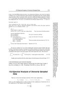
13.2 Correlation and Autocorrelation Using
the FFT
Correlation is the close mathematical cousin of convolution. It is in some
ways simpler, however, because the two functions that go into a correlation are not
as conceptually distinct as were the data and response functions that entered into
convolution. Rather, in correlation, the functions are represented by different, but
generally similar, data sets. We investigate their “correlation,” by comparing them
both directly superposed, and with one of them shifted left or right.
We have already defined in equation (12.0.10) the correlation between two
continuous functions g(t) and h(t), which is denoted Corr(g, h), and is a function
of lag t. We will occasionally show this time dependence explicitly, with the rather
awkward notation Corr(g, h)(t). The correlation will be large at some value of
t if the first function (g) is a close copy of the second (h) but lags it in time by
t, i.e., if the first function is shifted to the right of the second. Likewise, the
correlation will be large for some negative value of t if the first function leads the
second, i.e., is shifted to the left of the second. The relation that holds when the

two functions are interchanged is
Corr(g, h)(t)=Corr(h, g)(−t)(13.2.1)
The discrete correlation of two sampled functions g
k
and h
k
, each periodic
with period N,isdefinedby
Corr(g, h)
j
≡
N−1

k=0
g
j+k
h
k
(13.2.2)
The discrete correlation theorem says that this discrete correlation of two real
functions g and h is one member of the discrete Fourier transform pair
Corr(g, h)
j
⇐⇒ G
k
H
k
*(13.2.3)
where G
k

and H
k
are the discrete Fourier transforms of g
j
and h
j
, and the asterisk
denotes complex conjugation. This theorem makes the same presumptionsabout the
functions as those encountered for the discrete convolution theorem.
We can compute correlations using the FFT as follows: FFT the two data sets,
multiply one resulting transform by the complex conjugate of the other, and inverse
transform the product. The result (call it r
k
) will formally be a complex vector
of length N . However, it will turn out to have all its imaginary parts zero since
the original data sets were both real. The components of r
k
are the values of the
546
Chapter 13. Fourier and Spectral Applications
Sample page from NUMERICAL RECIPES IN C: THE ART OF SCIENTIFIC COMPUTING (ISBN 0-521-43108-5)
Copyright (C) 1988-1992 by Cambridge University Press.Programs Copyright (C) 1988-1992 by Numerical Recipes Software.
Permission is granted for internet users to make one paper copy for their own personal use. Further reproduction, or any copying of machine-
readable files (including this one) to any servercomputer, is strictly prohibited. To order Numerical Recipes books,diskettes, or CDROMs
visit website or call 1-800-872-7423 (North America only),or send email to (outside North America).
correlation at different lags, with positive and negative lags stored in the by now
familiar wrap-around order: The correlation at zero lag is in r
0
, the first component;
the correlation at lag 1 is in r

1
, the second component; the correlation at lag −1
is in r
N−1
, the last component; etc.
Just as in the case of convolution we have to consider end effects, since our
data will not, in general, be periodic as intended by the correlation theorem. Here
again, we can use zero padding. If you are interested in the correlation for lags as
large as ±K, then you must append a buffer zone of K zeros at the end of both
input data sets. If you want all possible lags from N data points (not a usual thing),
then you will need to pad the data with an equal number of zeros; this is the extreme
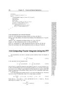
case. So here is the program:
#include "nrutil.h"
void correl(float data1[], float data2[], unsigned long n, float ans[])
Computes the correlation of two real data sets
data1[1 n] and data2[1 n] (including any
user-supplied zero padding).
n MUST be an integer power of two. The answer is returned as
the first
n points in ans[1 2*n] stored in wrap-around order, i.e., correlations at increasingly
negative lags are in
ans[n] on down to ans[n/2+1], while correlations at increasingly positive
lags are in
ans[1] (zerolag)onuptoans[n/2].Notethatans must be supplied in the calling
program with length at least
2*n, since it is also used as working space. Sign convention of
this routine: if
data1 lags data2, i.e., is shifted to the right of it, then ans will show a peak
at positive lags.
{

void realft(float data[], unsigned long n, int isign);
void twofft(float data1[], float data2[], float fft1[], float fft2[],
unsigned long n);
unsigned long no2,i;
float dum,*fft;
fft=vector(1,n<<1);
twofft(data1,data2,fft,ans,n); Transform b oth data vectors at once.
no2=n>>1; Normalization for inverse FFT.
for (i=2;i<=n+2;i+=2) {
ans[i-1]=(fft[i-1]*(dum=ans[i-1])+fft[i]*ans[i])/no2; Multiply to find
FFT of their cor-
relation.
ans[i]=(fft[i]*dum-fft[i-1]*ans[i])/no2;
}
ans[2]=ans[n+1]; Pack first and last into one element.
realft(ans,n,-1); Inverse transform gives correlation.
free_vector(fft,1,n<<1);
}
As in convlv, it would be better to substitute two calls to realft for the one
call to twofft,ifdata1 and data2 have very different magnitudes, to minimize
roundoff error.
The discrete autocorrelation of a sampled function g
j
is just the discrete
correlation of the function with itself. Obviously this is always symmetric with
respect to positive and negative lags. Feel free to use the above routine correl
to obtain autocorrelations, simply calling it with the same data vector in both
arguments. If the inefficiency bothers you, routine realft can,ofcourse,beused
to transform the data vector instead.
CITED REFERENCES AND FURTHER READING:

Brigham, E.O. 1974,
The Fast Fourier Transform
(Englewood Cliffs, NJ: Prentice-Hall), §13–2.
13.3 Optimal (Wiener) Filtering with the FFT
547
Sample page from NUMERICAL RECIPES IN C: THE ART OF SCIENTIFIC COMPUTING (ISBN 0-521-43108-5)
Copyright (C) 1988-1992 by Cambridge University Press.Programs Copyright (C) 1988-1992 by Numerical Recipes Software.
Permission is granted for internet users to make one paper copy for their own personal use. Further reproduction, or any copying of machine-
readable files (including this one) to any servercomputer, is strictly prohibited. To order Numerical Recipes books,diskettes, or CDROMs
visit website or call 1-800-872-7423 (North America only),or send email to (outside North America).
13.3 Optimal (Wiener) Filtering with the FFT
There are a number of other tasks in numerical processing that are routinely
handled with Fourier techniques. One of these is filtering for the removal of noise
from a “corrupted” signal. The particular situationwe consider is this: There is some
underlying, uncorrupted signal u(t) that we want to measure. The measurement
process is imperfect, however, and what comes out of our measurement device is a
corrupted signal c(t). The signal c(t) may be less than perfect in either or both of
two respects. First, the apparatus may not have a perfect “delta-function” response,
so that the true signal u(t) is convolved with (smeared out by) some known response
function r(t) to give a smeared signal s(t),
s(t)=

∞
−∞
r(t − τ)u(τ ) dτ or S(f)=R(f)U(f)(13.3.1)
where S, R, U are the Fourier transforms of s, r, u, respectively. Second, the
measured signal c(t) may contain an additional component of noise n(t),
c(t)=s(t)+n(t)(13.3.2)
We already know how to deconvolve the effects of the response function r in
the absence of any noise (§13.1); we just divide C(f) by R(f) to get a deconvolved

signal. We now want to treat the analogous problem when noise is present. Our
task is to find the optimal filter, φ(t) or Φ(f), which, when applied to the measured
signal c(t) or C(f), and then deconvolved by r(t) or R(f), produces a signal u(t)
or

U(f) that is as close as possible to the uncorrupted signal u(t) or U(f).Inother
words we will estimate the true signal U by

U(f)=
C(f)Φ(f)
R(f)
(13.3.3)
In what sense is

U to be close to U ? We ask that they be close in the
least-square sense

∞
−∞
|u(t) − u(t)|
2
dt =

∞
−∞




U(f) − U(f)




2
df is minimized. (13.3.4)
Substitutingequations (13.3.3) and (13.3.2), the right-hand side of (13.3.4) becomes

∞
−∞




[S(f)+N(f)]Φ(f)
R(f)
−
S(f)
R(f)




2
df
=

∞
−∞
|R(f)|
−2


|S(f)|
2
|1 − Φ(f)|
2
+ |N(f)|
2
|Φ(f)|
2

df
( 13.3.5)
The signal S and the noise N are uncorrelated, so their cross product, when
integrated over frequency f, gave zero. (This is practically the definition of what we
mean by noise!) Obviously (13.3.5) will be a minimum if and only if the integrand