Sensor Fusion and its Applications Part 8 pptx

Sensor Fusion and Its Applications204
4. References
Belongie, S., Malik, J. & Puzicha, J. (2002). Shape matching and object recognition using shape
contexts, IEEE Trans. Pattern Anal. Mach. Intell. Vol. 24(No. 4): 509–522.
Beringer, D. & Hancock, P. (1989). Summary of the various definitions of situation awareness,
Proc. of Fifth Intl. Symp. on Aviation Psychology Vol. 2(No.6): 646 – 651.
Bernardin, K., Ogawara, K., Ikeuchi, K. & Dillmann, R. (2003). A hidden markov model based
sensor fusion approach for recognizing continuous human grasping sequences, Proc.
3rd IEEE International Conference on Humanoid Robots pp. 1 – 13.
Bruckner, D., Sallans, B. & Russ, G. (2007). Hidden markov models for traffic observation,
Proc. 5th IEEE Intl. Conference on Industrial Informatics pp. 23 – 27.
Dalal, N. & Triggs, B. (2005). Histograms of oriented gradients for human detection, IEEE
Computer Society Conference on Computer Vision and Pattern Recognition (CVPR’05) Vol.
1: 886 – 893.
Damarla, T. (2008). Hidden markov model as a framework for situational awareness, Proc. of
Intl. Conference on Information Fusion, Cologne, Germany .
Damarla, T., Kaplan, L. & Chan, A. (2007). Human infrastructure & human activity detection,
Proc. of Intl. Conference on Information Fusion, Quebec City, Canada .
Damarla, T., Pham, T. & Lake, D. (2004). An algorithm for classifying multiple targets using
acoustic signatures, Proc. of SPIE Vol. 5429(No.): 421 – 427.
Damarla, T. & Ufford, D. (2007). Personnel detection using ground sensors, Proc. of SPIE Vol.
6562: 1 – 10.
Endsley, M. R. & Mataric, M. (2000). Situation Awareness Analysis and Measurement, Lawrence
Earlbaum Associates, Inc., Mahwah, New Jersey.
Green, M., Odom, J. & Yates, J. (1995). Measuring situational awareness with the ideal ob-
server, Proc. of the Intl. Conference on Experimental Analysis and Measurement of Situation
Awareness.
Hall, D. & Llinas, J. (2001). Handbook of Multisensor Data Fusion, CRC Press: Boca Raton.
HMM Toolbox (n.d.).
URL: www.cs.ubc.ca/~murphyk/Software/ HMM/hmm.html

Hough, P. V. C. (1962). Method and means for recognizing complex patterns, U.S. Patent
3069654 .
Houston, K. M. & McGaffigan, D. P. (2003). Spectrum analysis techniques for personnel de-
tection using seismic sensors, Proc. of SPIE Vol. 5090: 162 – 173.
Klein, L. A. (2004). Sensor and Data Fusion - A Tool for Information Assessment and Decision
Making, SPIE Press, Bellingham, Washington, USA.
Maj. Houlgate, K. P. (2004). Urban warfare transforms the corps, Proc. of the Naval Institute .
Pearl, J. (1986). Fusion, propagation, and structuring in belief networks, Artificial Intelligence
Vol. 29: 241 – 288.
Pearl, J. (1988). Probabilistic Reasoning in Intelligent Systems: Networks of Plausible Inference,
Morgan Kaufmann Publishers, Inc.
Press, D. G. (1998). Urban warfare: Options, problems and the future, Summary of a conference
sponsored by MIT Security Studies Program .
Rabiner, L. R. (1989). A tutorial on hidden markov models and selected applications in speech
recognition, Proc. of the IEEE Vol. 77(2): 257 – 285.
Sarter, N. B. & Woods, D. (1991). Situation awareness: A critical but ill-defined phenomenon,
Intl. Journal of Aviation Psychology Vol. 1: 45–57.
Singhal, A. & Brown, C. (1997). Dynamic bayes net approach to multimodal sensor fusion,
Proc. of SPIE Vol. 3209: 2 – 10.
Singhal, A. & Brown, C. (2000). A multilevel bayesian network approach to image sensor
fusion, Proc. ISIF, WeB3 pp. 9 – 16.
Smith, D. J. (2003). Situation(al) awareness (sa) in effective command and control, Wales .
Smith, K. & Hancock, P. A. (1995). The risk space representation of commercial airspace, Proc.
of the 8
th
Intl. Symposium on Aviation Psychology pp. 9 – 16.
Wang, L., Shi, J., Song, G. & Shen, I. (2007). Object detection combining recognition and
segmentation, Eighth Asian Conference on Computer Vision (ACCV) .
Hidden Markov Model as a Framework for Situational Awareness 205
4. References

Belongie, S., Malik, J. & Puzicha, J. (2002). Shape matching and object recognition using shape
contexts, IEEE Trans. Pattern Anal. Mach. Intell. Vol. 24(No. 4): 509–522.
Beringer, D. & Hancock, P. (1989). Summary of the various definitions of situation awareness,
Proc. of Fifth Intl. Symp. on Aviation Psychology Vol. 2(No.6): 646 – 651.
Bernardin, K., Ogawara, K., Ikeuchi, K. & Dillmann, R. (2003). A hidden markov model based
sensor fusion approach for recognizing continuous human grasping sequences, Proc.
3rd IEEE International Conference on Humanoid Robots pp. 1 – 13.
Bruckner, D., Sallans, B. & Russ, G. (2007). Hidden markov models for traffic observation,
Proc. 5th IEEE Intl. Conference on Industrial Informatics pp. 23 – 27.
Dalal, N. & Triggs, B. (2005). Histograms of oriented gradients for human detection, IEEE
Computer Society Conference on Computer Vision and Pattern Recognition (CVPR’05) Vol.
1: 886 – 893.
Damarla, T. (2008). Hidden markov model as a framework for situational awareness, Proc. of
Intl. Conference on Information Fusion, Cologne, Germany .
Damarla, T., Kaplan, L. & Chan, A. (2007). Human infrastructure & human activity detection,
Proc. of Intl. Conference on Information Fusion, Quebec City, Canada .
Damarla, T., Pham, T. & Lake, D. (2004). An algorithm for classifying multiple targets using
acoustic signatures, Proc. of SPIE Vol. 5429(No.): 421 – 427.
Damarla, T. & Ufford, D. (2007). Personnel detection using ground sensors, Proc. of SPIE Vol.
6562: 1 – 10.
Endsley, M. R. & Mataric, M. (2000). Situation Awareness Analysis and Measurement, Lawrence
Earlbaum Associates, Inc., Mahwah, New Jersey.
Green, M., Odom, J. & Yates, J. (1995). Measuring situational awareness with the ideal ob-
server, Proc. of the Intl. Conference on Experimental Analysis and Measurement of Situation
Awareness.
Hall, D. & Llinas, J. (2001). Handbook of Multisensor Data Fusion, CRC Press: Boca Raton.
HMM Toolbox (n.d.).
URL: www.cs.ubc.ca/~murphyk/Software/ HMM/hmm.html
Hough, P. V. C. (1962). Method and means for recognizing complex patterns, U.S. Patent
3069654 .

Houston, K. M. & McGaffigan, D. P. (2003). Spectrum analysis techniques for personnel de-
tection using seismic sensors, Proc. of SPIE Vol. 5090: 162 – 173.
Klein, L. A. (2004). Sensor and Data Fusion - A Tool for Information Assessment and Decision
Making, SPIE Press, Bellingham, Washington, USA.
Maj. Houlgate, K. P. (2004). Urban warfare transforms the corps, Proc. of the Naval Institute .
Pearl, J. (1986). Fusion, propagation, and structuring in belief networks, Artificial Intelligence
Vol. 29: 241 – 288.
Pearl, J. (1988). Probabilistic Reasoning in Intelligent Systems: Networks of Plausible Inference,
Morgan Kaufmann Publishers, Inc.
Press, D. G. (1998). Urban warfare: Options, problems and the future, Summary of a conference
sponsored by MIT Security Studies Program .
Rabiner, L. R. (1989). A tutorial on hidden markov models and selected applications in speech
recognition, Proc. of the IEEE Vol. 77(2): 257 – 285.
Sarter, N. B. & Woods, D. (1991). Situation awareness: A critical but ill-defined phenomenon,
Intl. Journal of Aviation Psychology Vol. 1: 45–57.
Singhal, A. & Brown, C. (1997). Dynamic bayes net approach to multimodal sensor fusion,
Proc. of SPIE Vol. 3209: 2 – 10.
Singhal, A. & Brown, C. (2000). A multilevel bayesian network approach to image sensor
fusion, Proc. ISIF, WeB3 pp. 9 – 16.
Smith, D. J. (2003). Situation(al) awareness (sa) in effective command and control, Wales .
Smith, K. & Hancock, P. A. (1995). The risk space representation of commercial airspace, Proc.
of the 8
th
Intl. Symposium on Aviation Psychology pp. 9 – 16.
Wang, L., Shi, J., Song, G. & Shen, I. (2007). Object detection combining recognition and
segmentation, Eighth Asian Conference on Computer Vision (ACCV) .
Sensor Fusion and Its Applications206
Multi-sensorial Active Perception for Indoor Environment Modeling 207
Multi-sensorial Active Perception for Indoor Environment Modeling
Luz Abril Torres-Méndez

X

Multi-sensorial Active Perception
for Indoor Environment Modeling

Luz Abril Torres-Méndez
Research Centre for Advanced Studies - Campus Saltillo
Mexico

1. Introduction
For many applications, the information provided by individual sensors is often incomplete,
inconsistent, or imprecise. For problems involving detection, recognition and reconstruction
tasks in complex environments, it is well known that no single source of information can
provide the absolute solution, besides the computational complexity. The merging of
multisource data can create a more consistent interpretation of the system of interest, in
which the associated uncertainty is decreased.
Multi-sensor data fusion also known simply as sensor data fusion is a process of combining
evidence from different information sources in order to make a better judgment (
Llinas &
Waltz, 1990; Hall, 1992; Klein, 1993)
. Although, the notion of data fusion has always been
around, most multisensory data fusion applications have been developed very recently,
converting it in an area of intense research in which new applications are being explored
constantly. On the surface, the concept of fusion may look to be straightforward but the
design and implementation of fusion systems is an extremely complex task. Modeling,
processing, and integrating of different sensor data for knowledge interpretation and
inference are challenging problems. These problems become even more difficult when the
available data is incomplete, inconsistent or imprecise.

In robotics and computer vision, the rapid advance of science and technology combined

with the reduction in the costs of sensor devices, has caused that these areas together, and
before considered as independent, strength the diverse needs of each. A central topic of
investigation in both areas is the recovery of the tridimensional structure of large-scale
environments. In a large-scale environment the complete scene cannot be captured from a
single referential frame or given position, thus an active way of capturing the information is
needed. In particular, having a mobile robot able to build a 3D map of the environment is
very appealing since it can be applied to many important applications. For example, virtual
exploration of remote places, either for security or efficiency reasons. These applications
depend not only on the correct transmission of visual and geometric information but also on
the quality of the information captured. The latter is closely related to the notion of active
perception as well as the uncertainty associated to each sensor. In particular, the behavior
any artificial or biological system should follow to accomplish certain tasks (e.g., extraction,
9
Sensor Fusion and Its Applications208

simplification and filtering), is strongly influenced by the data supplied by its sensors. This
data is in turn dependent on the perception criteria associated with each sensorial input
(Conde & Thalmann, 2004)
.

A vast body of research on 3D modeling and virtual reality applications has been focused on
the fusion of intensity and range data with promising results (Pulli et al., 1997; Stamos &
Allen, 2000) and recently (Guidi et al., 2009). Most of these works consider the complete
acquisition of 3D points from the object or scene to be modeled, focusing mainly on the
registration and integration problems.

In the area of computer vision, the idea of extracting the shape or structure from an image
has been studied since the end of the 70’s. Scientists in computer vision were mainly
interested in methods that reflect the way the human eye works. These methods, known as
“shape-from-X”, extract depth information by using visual patterns of the images, such as

shading, texture, binocular vision, motion, among others. Because of the type of sensors
used in these methods, they are categorized as passive sensing techniques, i.e., data is
obtained without emitting energy and involve typically mathematical models of the image
formation and how to invert them. Traditionally, these models are based on physical
principles of the light interaction. However, due to the difficulties to invert them, is
necessary to assume several aspects about the physical properties of the objects in the scene,
such as the type of surface (Lambertian, matte) and albedo, which cannot be suitable to real
complex scenes.

In the robotics community, it is common to combine information from different sensors,
even using the same sensors repeatedly over time, with the goal of building a model of the
environment. Depth inference is frequently achieved by using sophisticated, but costly,
hardware solutions. Range sensors, in particular laser rangefinders, are commonly used in
several applications due to its simplicity and reliability (but not its elegance, cost and
physical robustness). Besides of capturing 3D points in a direct and precise manner, range
measurements are independent of external lighting conditions. These techniques are known
as active sensing techniques. Although these techniques are particularly needed in non-
structured environments (e.g., natural outdoors, aquatic environments), they are not
suitable for capturing complete 2.5D maps with a resolution similar to that of a camera. The
reason for this is that these sensors are extremely expensive or, in other way, impractical,
since the data acquisition process may be slow and normally the spatial resolution of the
data is limited. On the other hand, intensity images have a high resolution which allows
precise results in well-defined objectives. These images are easy to acquire and give texture
maps in real color images.

However, although many elegant algorithms based on traditional approaches for depth
recovery have been developed, the fundamental problem of obtaining precise data is still a
difficult task. In particular, achieving geometric correctness and realism may require data
collection from different sensors as well as the correct fusion of all these observations.
Good examples are the stereo cameras that can produce volumetric scans that are

economical. However, these cameras require calibration or produce range maps that are
incomplete or of limited resolution. In general, using only 2D intensity images will provide

sparse measurements of the geometry which are non-reliable unless some simple geometry
about the scene to model is assumed. By fusing 2D intensity images with range finding
sensors, as first demonstrated in (Jarvis, 1992), a solution to 3D vision is realized -
circumventing the problem of inferring 3D from 2D.

One aspect of great importance in the 3D modeling reconstruction is to have a fast, efficient
and simple data acquisition process from the sensors and yet, have a good and robust
reconstruction. This is crucial when dealing with dynamic environments (e.g., people
walking around, illumination variation, etc.) and systems with limited battery-life. We can
simplify the way the data is acquired by capturing only partial but reliable range
information of regions of interest. In previous research work, the problem of tridimensional
scene recovery using incomplete sensorial data was tackled for the first time, specifically, by
using intensity images and a limited number of range data (Torres-Méndez & Dudek, 2003;
Torres-Méndez & Dudek, 2008). The main idea is based on the fact that the underlying
geometry of a scene can be characterized by the visual information and its interaction with
the environment together with its inter-relationships with the available range data. Figure 1
shows an example of how a complete and dense range map is estimated from an intensity
image and the associated partial depth map. These statistical relationships between the
visual and range data were analyzed in terms of small patches or neighborhoods of pixels,
showing that the contextual information of these relationships can provide information to
infer complete and dense range maps. The dense depth maps with their corresponding
intensity images are then used to build 3D models of large-scale man-made indoor
environments (offices, museums, houses, etc.)


Fig. 1. An example of the range synthesis process. The data fusion of intensity and
incomplete range is carried on to reconstruct a 3D model of the indoor scene. Image taken

from (Torres-Méndez, 2008).

In that research work, the sampling strategies for measuring the range data was determined
beforehand and remain fixed (vertical and horizontal lines through the scene) during the
data acquisition process. These sampling strategies sometimes carried on critical limitations
to get an ideal reconstruction as the quality of the input range data, in terms of the
geometric characteristics it represent, did not capture the underlying geometry of the scene
to be modeled. As a result, the synthesis process of the missing range data was very poor.
In the work presented in this chapter, we solve the above mentioned problem by selecting in
an optimal way the regions where the initial (minimal) range data must be captured. Here,
the term optimal refers in particular, to the fact that the range data to be measured must truly
Multi-sensorial Active Perception for Indoor Environment Modeling 209

simplification and filtering), is strongly influenced by the data supplied by its sensors. This
data is in turn dependent on the perception criteria associated with each sensorial input
(Conde & Thalmann, 2004)
.

A vast body of research on 3D modeling and virtual reality applications has been focused on
the fusion of intensity and range data with promising results (Pulli et al., 1997; Stamos &
Allen, 2000) and recently (Guidi et al., 2009). Most of these works consider the complete
acquisition of 3D points from the object or scene to be modeled, focusing mainly on the
registration and integration problems.

In the area of computer vision, the idea of extracting the shape or structure from an image
has been studied since the end of the 70’s. Scientists in computer vision were mainly
interested in methods that reflect the way the human eye works. These methods, known as
“shape-from-X”, extract depth information by using visual patterns of the images, such as
shading, texture, binocular vision, motion, among others. Because of the type of sensors
used in these methods, they are categorized as passive sensing techniques, i.e., data is

obtained without emitting energy and involve typically mathematical models of the image
formation and how to invert them. Traditionally, these models are based on physical
principles of the light interaction. However, due to the difficulties to invert them, is
necessary to assume several aspects about the physical properties of the objects in the scene,
such as the type of surface (Lambertian, matte) and albedo, which cannot be suitable to real
complex scenes.

In the robotics community, it is common to combine information from different sensors,
even using the same sensors repeatedly over time, with the goal of building a model of the
environment. Depth inference is frequently achieved by using sophisticated, but costly,
hardware solutions. Range sensors, in particular laser rangefinders, are commonly used in
several applications due to its simplicity and reliability (but not its elegance, cost and
physical robustness). Besides of capturing 3D points in a direct and precise manner, range
measurements are independent of external lighting conditions. These techniques are known
as active sensing techniques. Although these techniques are particularly needed in non-
structured environments (e.g., natural outdoors, aquatic environments), they are not
suitable for capturing complete 2.5D maps with a resolution similar to that of a camera. The
reason for this is that these sensors are extremely expensive or, in other way, impractical,
since the data acquisition process may be slow and normally the spatial resolution of the
data is limited. On the other hand, intensity images have a high resolution which allows
precise results in well-defined objectives. These images are easy to acquire and give texture
maps in real color images.

However, although many elegant algorithms based on traditional approaches for depth
recovery have been developed, the fundamental problem of obtaining precise data is still a
difficult task. In particular, achieving geometric correctness and realism may require data
collection from different sensors as well as the correct fusion of all these observations.
Good examples are the stereo cameras that can produce volumetric scans that are
economical. However, these cameras require calibration or produce range maps that are
incomplete or of limited resolution. In general, using only 2D intensity images will provide

sparse measurements of the geometry which are non-reliable unless some simple geometry
about the scene to model is assumed. By fusing 2D intensity images with range finding
sensors, as first demonstrated in (Jarvis, 1992), a solution to 3D vision is realized -
circumventing the problem of inferring 3D from 2D.

One aspect of great importance in the 3D modeling reconstruction is to have a fast, efficient
and simple data acquisition process from the sensors and yet, have a good and robust
reconstruction. This is crucial when dealing with dynamic environments (e.g., people
walking around, illumination variation, etc.) and systems with limited battery-life. We can
simplify the way the data is acquired by capturing only partial but reliable range
information of regions of interest. In previous research work, the problem of tridimensional
scene recovery using incomplete sensorial data was tackled for the first time, specifically, by
using intensity images and a limited number of range data (Torres-Méndez & Dudek, 2003;
Torres-Méndez & Dudek, 2008). The main idea is based on the fact that the underlying
geometry of a scene can be characterized by the visual information and its interaction with
the environment together with its inter-relationships with the available range data. Figure 1
shows an example of how a complete and dense range map is estimated from an intensity
image and the associated partial depth map. These statistical relationships between the
visual and range data were analyzed in terms of small patches or neighborhoods of pixels,
showing that the contextual information of these relationships can provide information to
infer complete and dense range maps. The dense depth maps with their corresponding
intensity images are then used to build 3D models of large-scale man-made indoor
environments (offices, museums, houses, etc.)


Fig. 1. An example of the range synthesis process. The data fusion of intensity and
incomplete range is carried on to reconstruct a 3D model of the indoor scene. Image taken
from (Torres-Méndez, 2008).

In that research work, the sampling strategies for measuring the range data was determined
beforehand and remain fixed (vertical and horizontal lines through the scene) during the
data acquisition process. These sampling strategies sometimes carried on critical limitations
to get an ideal reconstruction as the quality of the input range data, in terms of the
geometric characteristics it represent, did not capture the underlying geometry of the scene
to be modeled. As a result, the synthesis process of the missing range data was very poor.
In the work presented in this chapter, we solve the above mentioned problem by selecting in
an optimal way the regions where the initial (minimal) range data must be captured. Here,
the term optimal refers in particular, to the fact that the range data to be measured must truly
Sensor Fusion and Its Applications210

represent relevant information about the geometric structure. Thus, the input range data, in
this case, must be good enough to estimate, together with the visual information, the rest of
the missing range data.

Both sensors (camera and laser) must be fused (i.e., registered and then integrated) in a
common reference frame. The fusion of visual and range data involves a number of aspects
to be considered as the data is not of the same nature with respect to their resolution, type
and scale. The images of real scene, i.e., those that represent a meaningful concept in their
content, depend on the regularities of the environment in which they are captured (Van Der
Schaaf, 1998). These regularities can be, for example, the natural geometry of objects and
their distribution in space; the natural distributions of light; and the regularities that depend
on the viewer’s position. This is particularly difficult considering the fact that at each given
position the mobile robot must capture a number of images and then analyze the optimal
regions where the range data should be measured. This means that the laser should be
directed to those regions with accuracy and then the incomplete range data must be
registered with the intensity images before applying the statistical learning method to
estimate complete and dense depth maps.
The statistical studies of these images can help to understand these regularities, which are
not easily acquired from physical or mathematical models. Recently, there has been some

success when using statistical methods to computer vision problems (Freeman & Torralba,
2002; Srivastava et al., 2003; Torralba & Oliva, 2002). However, more studies are needed in
the analysis of the statistical relationships between intensity and range data. Having
meaningful statistical tendencies could be of great utility in the design of new algorithms to
infer the geometric structure of objects in a scene.

The outline of the chapter is as follows. In Section 2 we present related work to the problem
of 3D environment modeling focusing on approaches that fuse intensity and range images.
Section 3 presents our multi-sensorial active perception framework which statistically
analyzes natural and indoor images to capture the initial range data. This range data
together with the available intensity will be used to efficiently estimate dense range maps.
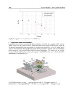
Experimental results under different scenarios are shown in Section 4 together with an
evaluation of the performance of the method.

2. Related Work
For the fundamental problem in computer vision of recovering the geometric structure of
objects from 2D images, different monocular visual cues have been used, such as shading,
defocus, texture, edges, etc. With respect to binocular visual cues, the most common are the
obtained from stereo cameras, from which we can compute a depth map in a fast and
economical way. For example, the method proposed in (Wan & Zhou, 2009), uses stereo
vision as a basis to estimate dense depth maps of large-scale scenes. They generate depth
map mosaics, with different angles and resolutions which are combined later in a single
large depth map. The method presented in (Malik and Choi, 2008) is based in the shape
from focus approach and use a defocus measure based in an optic transfer function
implemented in the Fourier domain. In (Miled & Pesquet, 2009), the authors present a novel
method based on stereo that help to estimate depth maps of scene that are subject to changes

in illumination. Other works propose to combine different methods to obtain the range
maps. For example, in (Scharstein & Szeliski, 2003) a stereo vision algorithm and structured
light are used to reconstruct scenes in 3D. However, the main disadvantage of above

techniques is that the obtained range maps are usually incomplete or of limited resolution
and in most of the cases a calibration is required.

Another way of obtaining a dense depth map is by using range sensors (e.g., laser scanners),
which obtain geometric information in a direct and reliable way. A large number of possible
3D scanners are available on the market. However, cost is still the major concern and the
more economical tend to be slow. An overview of different systems available to 3D shape of
objects is presented in (Blais, 2004), highlighting some of the advantages and disadvantages
of the different methods. Laser Range Finders directly map the acquired data into a 3D
volumetric model thus having the ability to partly avoid the correspondence problem
associated with visual passive techniques. Indeed, scenes with no textural details can be
easily modeled. Moreover, laser range measurements do not depend on scene illumination.

More recently, techniques based on learning statistics have been used to recover the
geometric structure from 2D images. For humans, to interpret the geometric information of
a scene by looking to one image is not a difficult task. However, for a computational
algorithm this is difficult as some a priori knowledge about the scene is needed.
For example, in (Torres-Méndez & Dudek, 2003) it was presented for the first time a method
to estimate dense range map based on the statistical correlation between intensity and
available range as well as edge information. Other studies developed more recently as in
(Saxena & Chung, 2008), show that it is possible to recover the missing range data in the
sparse depth maps using statistical learning approaches together with the appropriate
characteristics of objects in the scene (e.g., edges or cues indicating changes in depth). Other
works combine different types of visual cues to facilitate the recovery of depth information
or the geometry of objects of interest.
In general, no matter what approach is used, the quality of the results will strongly depend
on the type of visual cues used and the preprocessing algorithms applied to the input data.

3. The Multi-sensorial Active Perception Framework
This research work focuses on recovering the geometric (depth) information of a man-made

indoor scene (e.g., an office, a room) by fusing photometric and partial geometric
information in order to build a 3D model of the environment.
Our data fusion framework is based on an active perception technique that captures the
limited range data in regions statistically detected from the intensity images of the same
scene. In order to do that, a perfect registration between the intensity and range data is
required. The registration process we use is briefly described in Section 3.2. After
registering the partial range with the intensity data we apply a statistical learning method to
estimate the unknown range and obtain a dense range map. As the mobile robot moves at
different locations to capture information from the scene, the final step is to integrate all the
dense range maps (together with intensity) and build a 3D map of the environment.

Multi-sensorial Active Perception for Indoor Environment Modeling 211

represent relevant information about the geometric structure. Thus, the input range data, in
this case, must be good enough to estimate, together with the visual information, the rest of
the missing range data.

Both sensors (camera and laser) must be fused (i.e., registered and then integrated) in a
common reference frame. The fusion of visual and range data involves a number of aspects
to be considered as the data is not of the same nature with respect to their resolution, type
and scale. The images of real scene, i.e., those that represent a meaningful concept in their
content, depend on the regularities of the environment in which they are captured (Van Der
Schaaf, 1998). These regularities can be, for example, the natural geometry of objects and
their distribution in space; the natural distributions of light; and the regularities that depend
on the viewer’s position. This is particularly difficult considering the fact that at each given
position the mobile robot must capture a number of images and then analyze the optimal
regions where the range data should be measured. This means that the laser should be
directed to those regions with accuracy and then the incomplete range data must be
registered with the intensity images before applying the statistical learning method to
estimate complete and dense depth maps.

The statistical studies of these images can help to understand these regularities, which are
not easily acquired from physical or mathematical models. Recently, there has been some
success when using statistical methods to computer vision problems (Freeman & Torralba,
2002; Srivastava et al., 2003; Torralba & Oliva, 2002). However, more studies are needed in
the analysis of the statistical relationships between intensity and range data. Having
meaningful statistical tendencies could be of great utility in the design of new algorithms to
infer the geometric structure of objects in a scene.

The outline of the chapter is as follows. In Section 2 we present related work to the problem
of 3D environment modeling focusing on approaches that fuse intensity and range images.
Section 3 presents our multi-sensorial active perception framework which statistically
analyzes natural and indoor images to capture the initial range data. This range data
together with the available intensity will be used to efficiently estimate dense range maps.
Experimental results under different scenarios are shown in Section 4 together with an
evaluation of the performance of the method.

2. Related Work
For the fundamental problem in computer vision of recovering the geometric structure of
objects from 2D images, different monocular visual cues have been used, such as shading,
defocus, texture, edges, etc. With respect to binocular visual cues, the most common are the
obtained from stereo cameras, from which we can compute a depth map in a fast and
economical way. For example, the method proposed in (Wan & Zhou, 2009), uses stereo
vision as a basis to estimate dense depth maps of large-scale scenes. They generate depth
map mosaics, with different angles and resolutions which are combined later in a single
large depth map. The method presented in (Malik and Choi, 2008) is based in the shape
from focus approach and use a defocus measure based in an optic transfer function
implemented in the Fourier domain. In (Miled & Pesquet, 2009), the authors present a novel
method based on stereo that help to estimate depth maps of scene that are subject to changes

in illumination. Other works propose to combine different methods to obtain the range

maps. For example, in (Scharstein & Szeliski, 2003) a stereo vision algorithm and structured
light are used to reconstruct scenes in 3D. However, the main disadvantage of above
techniques is that the obtained range maps are usually incomplete or of limited resolution
and in most of the cases a calibration is required.

Another way of obtaining a dense depth map is by using range sensors (e.g., laser scanners),
which obtain geometric information in a direct and reliable way. A large number of possible
3D scanners are available on the market. However, cost is still the major concern and the
more economical tend to be slow. An overview of different systems available to 3D shape of
objects is presented in (Blais, 2004), highlighting some of the advantages and disadvantages
of the different methods. Laser Range Finders directly map the acquired data into a 3D
volumetric model thus having the ability to partly avoid the correspondence problem
associated with visual passive techniques. Indeed, scenes with no textural details can be
easily modeled. Moreover, laser range measurements do not depend on scene illumination.

More recently, techniques based on learning statistics have been used to recover the
geometric structure from 2D images. For humans, to interpret the geometric information of
a scene by looking to one image is not a difficult task. However, for a computational
algorithm this is difficult as some a priori knowledge about the scene is needed.
For example, in (Torres-Méndez & Dudek, 2003) it was presented for the first time a method
to estimate dense range map based on the statistical correlation between intensity and
available range as well as edge information. Other studies developed more recently as in
(Saxena & Chung, 2008), show that it is possible to recover the missing range data in the
sparse depth maps using statistical learning approaches together with the appropriate
characteristics of objects in the scene (e.g., edges or cues indicating changes in depth). Other
works combine different types of visual cues to facilitate the recovery of depth information
or the geometry of objects of interest.
In general, no matter what approach is used, the quality of the results will strongly depend
on the type of visual cues used and the preprocessing algorithms applied to the input data.

3. The Multi-sensorial Active Perception Framework
This research work focuses on recovering the geometric (depth) information of a man-made
indoor scene (e.g., an office, a room) by fusing photometric and partial geometric
information in order to build a 3D model of the environment.
Our data fusion framework is based on an active perception technique that captures the
limited range data in regions statistically detected from the intensity images of the same
scene. In order to do that, a perfect registration between the intensity and range data is
required. The registration process we use is briefly described in Section 3.2. After
registering the partial range with the intensity data we apply a statistical learning method to
estimate the unknown range and obtain a dense range map. As the mobile robot moves at
different locations to capture information from the scene, the final step is to integrate all the
dense range maps (together with intensity) and build a 3D map of the environment.

Sensor Fusion and Its Applications212

The key role of our active perception process concentrates on capturing range data from
places where the visual cues of the images show depth discontinuities. Man-made indoor
environments have inherent geometric and photometric characteristics that can be exploited
to help in the detection of this type of visual cues.

First, we apply a statistical analysis on an image database to detect regions of interest on
which range data should be acquired. With the internal representation, we can assign
confidence values according to the ternary values obtained. These values will indicate the
filling order of the missing range values. And finally, we use a non-parametric range
synthesis method in (Torres-Méndez & Dudek, 2003) to estimate the missing range values
and obtain a dense depth map. In the following sections, all these stages are explained in
more detail.

3.1 Detecting regions of interest from intensity images
We wish to capture limited range data in order to simplify the data acquisition process.

However, in order to have a good estimation of the unknown range, the quality of this
initial range data is crucial. That is, it should represent the depth discontinuities existing in
the scene. Since we have only information from images, we can apply a statistical analysis
on the images and extract changes in depth.

Given that our method is based on a statistical analysis, the type of images to analyze in the
database must contain characteristics and properties similar to the scenes of interest, as we
focus on man-made scenes, we should have images containing those types of images.
However, we start our experiments using a public available image database, the van
Hateren database, which contains scenes of natural images. As this database contains
important changes in depth in their scenes, this turns out to be the main characteristic to be
considered so that our method can be functional.

The statistical analysis of small patches implemented is based in part on the Feldman and
Yunes algorithm (Feldman & Yunes, 2006). This algorithm extracts characteristics of interest
from an image through the observation of an image database and obtains an internal
representation that concentrates the relevant information in a form of a ternary variable. To
generate the internal representation we follow three steps. First, we reduce (in scale) the
images in the database (see Figure 2). Then, each image is divided in patches of same size
(e.g. 13 x13 pixels), with these patches we make a new database which is decomposed in its
principal components by applying PCA to extract the most representative information,
which is usually contained, in the first five eigenvectors. In Figure 3, the eigenvectors are
depicted. These eigenvectors are the filters that are used to highlight certain characteristics
on the intensity images, specifically the regions with relevant geometric information.
The last step consists on applying a threshold in order to map the images onto a ternary
variable where we assign -1 value to very low values, 1 to high values and 0 otherwise. This
way, we can obtain an internal representation


k

i
G }1,0,1{: 

, (1)


where k represents the number of filters (eigenvectors). G is the set of pixels of the scaled
image.


Fig. 2. Some of the images taken from the van Hateren database. These images are reduced
by a scaled factor of 2.


Fig. 3. The first 5 eigenvectors (zoomed out). These eigenvectors are used as filters to
highlight relevant geometric information.

The internal representation gives information about the changes in depth as it is shown in
Figure 4. It can be observed that, depending on the filter used, the representation gives a
different orientation on the depth discontinuities in the scene. For example, if we use the
first filter, the highlighted changes are the horizontal ones. If we applied the second filter,
the discontinuities obtained are the vertical ones.



Fig. 4. The internal representation after the input image is filtered.

This internal representation is the basis to capture the initial range data from which we can
obtain a dense range map.

3.2 Obtaining the registered sparse depth map
In order to obtain the initial range data we need to register the camera and laser sensors, i.e.,
the corresponding reference frame of the intensity image taken from the camera with the
reference frame of the laser rangefinder. Our data acquisition system consists of a high
resolution digital camera and a 2D laser rangefinder (laser scanner), both mounted on a pan
unit and on top of a mobile robot. Registering different types of sensor data, which have
different projections, resolutions and scaling properties is a difficult task. The simplest and
easiest way to facilitate this sensor-to-sensor registration is to vertically align their center of
projections (optical center for the camera and mirror center for the laser) are aligned to the
center of projection of the pan unit. Thus, both sensors can be registered with respect to a
common reference frame. The laser scanner and camera sensors work with different
coordinate systems and they must be adjusted one to another. The laser scanner delivers
spherical coordinates whereas the camera puts out data in a typical image projection. Once
the initial the range data is collected we apply a post-registration algorithm which uses their
projection types in order to do an image mapping.
Multi-sensorial Active Perception for Indoor Environment Modeling 213

The key role of our active perception process concentrates on capturing range data from
places where the visual cues of the images show depth discontinuities. Man-made indoor
environments have inherent geometric and photometric characteristics that can be exploited
to help in the detection of this type of visual cues.

First, we apply a statistical analysis on an image database to detect regions of interest on
which range data should be acquired. With the internal representation, we can assign
confidence values according to the ternary values obtained. These values will indicate the
filling order of the missing range values. And finally, we use a non-parametric range
synthesis method in (Torres-Méndez & Dudek, 2003) to estimate the missing range values
and obtain a dense depth map. In the following sections, all these stages are explained in
more detail.

3.1 Detecting regions of interest from intensity images
We wish to capture limited range data in order to simplify the data acquisition process.
However, in order to have a good estimation of the unknown range, the quality of this
initial range data is crucial. That is, it should represent the depth discontinuities existing in
the scene. Since we have only information from images, we can apply a statistical analysis
on the images and extract changes in depth.

Given that our method is based on a statistical analysis, the type of images to analyze in the
database must contain characteristics and properties similar to the scenes of interest, as we
focus on man-made scenes, we should have images containing those types of images.
However, we start our experiments using a public available image database, the van
Hateren database, which contains scenes of natural images. As this database contains
important changes in depth in their scenes, this turns out to be the main characteristic to be
considered so that our method can be functional.

The statistical analysis of small patches implemented is based in part on the Feldman and
Yunes algorithm (Feldman & Yunes, 2006). This algorithm extracts characteristics of interest
from an image through the observation of an image database and obtains an internal
representation that concentrates the relevant information in a form of a ternary variable. To
generate the internal representation we follow three steps. First, we reduce (in scale) the
images in the database (see Figure 2). Then, each image is divided in patches of same size
(e.g. 13 x13 pixels), with these patches we make a new database which is decomposed in its
principal components by applying PCA to extract the most representative information,
which is usually contained, in the first five eigenvectors. In Figure 3, the eigenvectors are
depicted. These eigenvectors are the filters that are used to highlight certain characteristics
on the intensity images, specifically the regions with relevant geometric information.
The last step consists on applying a threshold in order to map the images onto a ternary
variable where we assign -1 value to very low values, 1 to high values and 0 otherwise. This
way, we can obtain an internal representation

k
i
G }1,0,1{: 

, (1)


where k represents the number of filters (eigenvectors). G is the set of pixels of the scaled
image.


Fig. 2. Some of the images taken from the van Hateren database. These images are reduced
by a scaled factor of 2.


Fig. 3. The first 5 eigenvectors (zoomed out). These eigenvectors are used as filters to
highlight relevant geometric information.

The internal representation gives information about the changes in depth as it is shown in
Figure 4. It can be observed that, depending on the filter used, the representation gives a
different orientation on the depth discontinuities in the scene. For example, if we use the
first filter, the highlighted changes are the horizontal ones. If we applied the second filter,
the discontinuities obtained are the vertical ones.



Fig. 4. The internal representation after the input image is filtered.

This internal representation is the basis to capture the initial range data from which we can

obtain a dense range map.

3.2 Obtaining the registered sparse depth map
In order to obtain the initial range data we need to register the camera and laser sensors, i.e.,
the corresponding reference frame of the intensity image taken from the camera with the
reference frame of the laser rangefinder. Our data acquisition system consists of a high
resolution digital camera and a 2D laser rangefinder (laser scanner), both mounted on a pan
unit and on top of a mobile robot. Registering different types of sensor data, which have
different projections, resolutions and scaling properties is a difficult task. The simplest and
easiest way to facilitate this sensor-to-sensor registration is to vertically align their center of
projections (optical center for the camera and mirror center for the laser) are aligned to the
center of projection of the pan unit. Thus, both sensors can be registered with respect to a
common reference frame. The laser scanner and camera sensors work with different
coordinate systems and they must be adjusted one to another. The laser scanner delivers
spherical coordinates whereas the camera puts out data in a typical image projection. Once
the initial the range data is collected we apply a post-registration algorithm which uses their
projection types in order to do an image mapping.
Sensor Fusion and Its Applications214

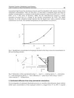
The image-based registration algorithm is similar to that presented in (Torres-Méndez &
Dudek, 2008) and assumes that the optical center of the camera and the mirror center of the
laser scanner are vertically aligned and the orientation of both rotation axes coincide (see
Figure 5). Thus, we only need to transform the panoramic camera data into the laser
coordinate system. Details of the algorithm we use are given in (Torres-Méndez & Dudek,
2008).


Fig. 5. Camera and laser scanner orientation and world coordinate system. Image taken
from (Torres-Méndez & Dudek, 2008).

3.3 The range synthesis method
After obtaining the internal representation and a registered sparse depth map, we can apply
the range synthesis method in (Torres-Méndez & Dudek, 2008). In general, the method
estimates dense depth maps using intensity and partial range information. The Markov
Random Field (MRF) model is trained using the (local) relationships between the observed
range data and the variations in the intensity images and then used to compute the
unknown range values. The Markovianity condition describes the local characteristics of the
pixel values (in intensity and range, called voxels). The range value at a voxel depends only
on neighboring voxels which have direct interactions on each other. We describe the non-
parametric method in general and skip the details of the basis of MRF; the reader is referred
to (Torres-Méndez & Dudek, 2008) for further details.

In order to compute the maximum a posteriori (MAP) for a depth value R
i
of a voxel V
i
, we
need first to build an approximate distribution of the conditional probability P(f
i
 f
Ni
) and
sample from it. For each new depth value R
i
 R to estimate, the samples that correspond to



Fig. 6. A sketch of the neighborhood system definition.

the neighborhood system of voxel i, i.e., N
i
, are taken and the distribution of R
i
is built as a
histogram of all possible values that occur in the sample. The neighborhood system N
i
(see
Figure 6) is an infinite real subset of voxels, denoted by N
real
. Taking the MRF model as a
basis, it is assumed that the depth value R
i
depends only on the intensity and range values
of its immediate neighbors defined in N
i
. If we define a set

},0:{)(
**
 NNNR
ireali
N (2)

that contains all occurrences of N
i
in N
real
, then the conditional probability distribution of R
i

can be estimated through a histogram based on the depth values of voxels representing each
N
i
in (R
i
). Unfortunately, the sample is finite and there exists the possibility that no
neighbor has exactly the same characteristics in intensity and range, for that reason we use
the heuristic of finding the most similar value in the available finite sample ’(R
i
), where
’(R
i
)  (R
i
). Now, let A
p
be a local neighborhood system for voxel p, which is composed
for neighbors that are located within radius r and is defined as:


}.),(dist { rqpNAA
qp

(3)

In the non-parametric approximation, the depth value R
p
of voxel V
p

with neighborhood N
p
,
is synthesized by selecting the most similar neighborhood N
best
to N
p
.


. , minarg
pqpbest
AAANN
q

(4)

All neighborhoods A
q
in A
p
that are similar to N
best
are included in ’(R
p
) as follows:


 
. 1

bestpqp
NNAN 

(5)

The similarity measure between two neighborhoods N
a
and N
b
is described over the partial
data of the two neighborhoods and is calculated as follows:

Multi-sensorial Active Perception for Indoor Environment Modeling 215

The image-based registration algorithm is similar to that presented in (Torres-Méndez &
Dudek, 2008) and assumes that the optical center of the camera and the mirror center of the
laser scanner are vertically aligned and the orientation of both rotation axes coincide (see
Figure 5). Thus, we only need to transform the panoramic camera data into the laser
coordinate system. Details of the algorithm we use are given in (Torres-Méndez & Dudek,
2008).


Fig. 5. Camera and laser scanner orientation and world coordinate system. Image taken
from (Torres-Méndez & Dudek, 2008).

3.3 The range synthesis method
After obtaining the internal representation and a registered sparse depth map, we can apply
the range synthesis method in (Torres-Méndez & Dudek, 2008). In general, the method
estimates dense depth maps using intensity and partial range information. The Markov
Random Field (MRF) model is trained using the (local) relationships between the observed

range data and the variations in the intensity images and then used to compute the
unknown range values. The Markovianity condition describes the local characteristics of the
pixel values (in intensity and range, called voxels). The range value at a voxel depends only
on neighboring voxels which have direct interactions on each other. We describe the non-
parametric method in general and skip the details of the basis of MRF; the reader is referred
to (Torres-Méndez & Dudek, 2008) for further details.

In order to compute the maximum a posteriori (MAP) for a depth value R
i
of a voxel V
i
, we
need first to build an approximate distribution of the conditional probability P(f
i
 f
Ni
) and
sample from it. For each new depth value R
i
 R to estimate, the samples that correspond to



Fig. 6. A sketch of the neighborhood system definition.

the neighborhood system of voxel i, i.e., N
i
, are taken and the distribution of R
i
is built as a

histogram of all possible values that occur in the sample. The neighborhood system N
i
(see
Figure 6) is an infinite real subset of voxels, denoted by N
real
. Taking the MRF model as a
basis, it is assumed that the depth value R
i
depends only on the intensity and range values
of its immediate neighbors defined in N
i
. If we define a set


},0:{)(
**
 NNNR
ireali
N (2)

that contains all occurrences of N
i
in N
real
, then the conditional probability distribution of R
i

can be estimated through a histogram based on the depth values of voxels representing each
N
i

in (R
i
). Unfortunately, the sample is finite and there exists the possibility that no
neighbor has exactly the same characteristics in intensity and range, for that reason we use
the heuristic of finding the most similar value in the available finite sample ’(R
i
), where
’(R
i
)  (R
i
). Now, let A
p
be a local neighborhood system for voxel p, which is composed
for neighbors that are located within radius r and is defined as:


}.),(dist { rqpNAA
qp

(3)

In the non-parametric approximation, the depth value R
p
of voxel V
p
with neighborhood N
p
,
is synthesized by selecting the most similar neighborhood N

best
to N
p
.


. , minarg
pqpbest
AAANN
q

(4)

All neighborhoods A
q
in A
p
that are similar to N
best
are included in ’(R
p
) as follows:


 
. 1
bestpqp
NNAN 

(5)

The similarity measure between two neighborhoods N
a
and N
b
is described over the partial
data of the two neighborhoods and is calculated as follows:

Sensor Fusion and Its Applications216


Fig. 7. The notation diagram. Taken from (Torres-Méndez, 2008).








ba
NNv
ba
DvvGNN
,
0
,





(6)






,
22
b
v
a
v
b
v
a
v
RRIID

 (7)

where
0
v

represents the voxel located in the center of the neighborhood N
a
and N
b

, v

is the
neighboring pixel of
0
v

. I
a
and R
a
are the intensity and range values to be compared. G is a
Gaussian kernel that is applied to each neighborhood so that voxels located near the center
have more weight that those located far from it. In this way we can build a histogram of
depth values R
p
in the center of each neighborhood in ’(R
i
).

3.3.1 Computing the priority values to establish the filling order
To achieve a good estimation for the unknown depth values, it is critical to establish an
order to select the next voxel to synthesize. We base this order on the amount of available
information at each voxel’s neighborhood, so that the voxel with more neighboring voxels
with already assigned intensity and range is synthesized first. We have observed that the
reconstruction in areas with discontinuities is very problematic and a probabilistic inference
is needed in these regions. Fortunately, such regions are identified by our internal
representation (described in Section 3.1) and can be used to assign priority values. For
example, we assign a high priority to voxels which ternary value is 1, so these voxels are
synthesized first; and a lower priority to voxels with ternary value 0 and -1, so they are

synthesized at the end.
The region to be synthesized is indicated by ={w
i
 iA}, where w
i
= R(x
i
,y
i
) is the unknown
depth value located at pixel coordinates (x
i
,y
i
). The input intensity and the known range
value together conform the source region and is indicated by  (see Figure 6). This region is
used to calculate the statistics between the input intensity and range for the reconstruction.
If V
p
is the voxel with an unknown range value, inside  and N
p
is its neighborhood, which

is an nxn window centered at V
p
, then for each voxel V
p
, we calculate its priority value as
follows

,
1
)()(
)(




p
Ni
ii
p
N
VFVC
VP
p
(8)

where

.
 indicates the total number of voxels in N
p
. Initially, the priority value of C(V
i
) for
each voxel V
p
 is assigned a value of 1 if the associated ternary value is 1, 0.8 if its ternary

value is 0 and 0.2 if -1. F(V
i
) is a flag function, which takes value 1 if the intensity and range
values of V
i
are known, and 0 if its range value is unknown. In this way, voxels with greater
priority are synthesized first.

3.4 Integration of dense range maps
We have mentioned that at each position the mobile robot takes an image, computes its
internal representation to direct the laser range finder on the regions detected and capture
range data. In order to produce a complete 3D model or representation of a large
environment, we need to integrate dense panoramas with depth from multiple viewpoints.
The approach taken is based on a hybrid method similar to that in (Torres-Méndez &
Dudek, 2008) (the reader is advised to refer to the article for further details).
In general, the integration algorithm combines a geometric technique, which is a variant of
the ICP algorithm (Besl & McKay, 1992) that matches 3D range scans, and an image-based
technique, the SIFT algorithm (Lowe, 1999), that matches intensity features on the images.
Since dense range maps with its corresponding intensity images are given as an input, their
integration to a common reference frame is easier than having only intensity or range data
separately.

4. Experimental Results
In order to evaluate the performance of the method, we use three databases, two of which
are available on the web. One is the Middlebury database (Hiebert-Treuer, 2008) which
contains intensity and dense range maps of 12 different indoor scenes containing objects
with a great variety of texture. The other is the USF database from the CESAR lab at Oak
Ridge National Laboratory. This database has intensity and dense range maps of indoor
scenes containing regular geometric objects with uniform textures. The third database was
created by capturing images using a stereo vision system in our laboratory. The scenes

contain regular geometric objects with different textures. As we have ground truth range
data from the public databases, we first simulate sparse range maps by eliminating some of
the range information using different sampling strategies that follows different patterns
(squares, vertical and horizontal lines, etc.) The sparse depth maps are then given as an
input to our algorithm to estimate dense range maps. In this way, we can compare the
ground-truth dense range maps with those synthesized by our method and obtain a quality
measure for the reconstruction.
Multi-sensorial Active Perception for Indoor Environment Modeling 217


Fig. 7. The notation diagram. Taken from (Torres-Méndez, 2008).








ba
NNv
ba
DvvGNN
,
0
,





(6)






,
22
b
v
a
v
b
v
a
v
RRIID

 (7)

where
0
v

represents the voxel located in the center of the neighborhood N
a
and N
b
, v


is the
neighboring pixel of
0
v

. I
a
and R
a
are the intensity and range values to be compared. G is a
Gaussian kernel that is applied to each neighborhood so that voxels located near the center
have more weight that those located far from it. In this way we can build a histogram of
depth values R
p
in the center of each neighborhood in ’(R
i
).

3.3.1 Computing the priority values to establish the filling order
To achieve a good estimation for the unknown depth values, it is critical to establish an
order to select the next voxel to synthesize. We base this order on the amount of available
information at each voxel’s neighborhood, so that the voxel with more neighboring voxels
with already assigned intensity and range is synthesized first. We have observed that the
reconstruction in areas with discontinuities is very problematic and a probabilistic inference
is needed in these regions. Fortunately, such regions are identified by our internal
representation (described in Section 3.1) and can be used to assign priority values. For
example, we assign a high priority to voxels which ternary value is 1, so these voxels are
synthesized first; and a lower priority to voxels with ternary value 0 and -1, so they are
synthesized at the end.

The region to be synthesized is indicated by ={w
i
 iA}, where w
i
= R(x
i
,y
i
) is the unknown
depth value located at pixel coordinates (x
i
,y
i
). The input intensity and the known range
value together conform the source region and is indicated by  (see Figure 6). This region is
used to calculate the statistics between the input intensity and range for the reconstruction.
If V
p
is the voxel with an unknown range value, inside  and N
p
is its neighborhood, which

is an nxn window centered at V
p
, then for each voxel V
p
, we calculate its priority value as
follows

,
1
)()(
)(




p
Ni
ii
p
N
VFVC
VP
p
(8)

where

.
 indicates the total number of voxels in N
p
. Initially, the priority value of C(V
i
) for
each voxel V
p
 is assigned a value of 1 if the associated ternary value is 1, 0.8 if its ternary
value is 0 and 0.2 if -1. F(V

i
) is a flag function, which takes value 1 if the intensity and range
values of V
i
are known, and 0 if its range value is unknown. In this way, voxels with greater
priority are synthesized first.

3.4 Integration of dense range maps
We have mentioned that at each position the mobile robot takes an image, computes its
internal representation to direct the laser range finder on the regions detected and capture
range data. In order to produce a complete 3D model or representation of a large
environment, we need to integrate dense panoramas with depth from multiple viewpoints.
The approach taken is based on a hybrid method similar to that in (Torres-Méndez &
Dudek, 2008) (the reader is advised to refer to the article for further details).
In general, the integration algorithm combines a geometric technique, which is a variant of
the ICP algorithm (Besl & McKay, 1992) that matches 3D range scans, and an image-based
technique, the SIFT algorithm (Lowe, 1999), that matches intensity features on the images.
Since dense range maps with its corresponding intensity images are given as an input, their
integration to a common reference frame is easier than having only intensity or range data
separately.

4. Experimental Results
In order to evaluate the performance of the method, we use three databases, two of which
are available on the web. One is the Middlebury database (Hiebert-Treuer, 2008) which
contains intensity and dense range maps of 12 different indoor scenes containing objects
with a great variety of texture. The other is the USF database from the CESAR lab at Oak
Ridge National Laboratory. This database has intensity and dense range maps of indoor
scenes containing regular geometric objects with uniform textures. The third database was
created by capturing images using a stereo vision system in our laboratory. The scenes
contain regular geometric objects with different textures. As we have ground truth range

data from the public databases, we first simulate sparse range maps by eliminating some of
the range information using different sampling strategies that follows different patterns
(squares, vertical and horizontal lines, etc.) The sparse depth maps are then given as an
input to our algorithm to estimate dense range maps. In this way, we can compare the
ground-truth dense range maps with those synthesized by our method and obtain a quality
measure for the reconstruction.
Sensor Fusion and Its Applications218

To evaluate our results we compute a well-know metric, called mean absolute residual
(MAR) error. The MAR error of two matrices R
1
and R
2
is defined as






voxelsrangeunknown #
,
21
,,
MAR



ji
jiRjiR

(9)

In general, just computing the MAR error is not a good mechanism to evaluate the success
of the method. For example, when there are few results with a high MAR error, the average
of the MAR error elevates. For this reason, we also compute the absolute difference at each
pixel and show the result as an image, so we can visually evaluate our performance.
In all the experiments, the size of the neighborhood N is 3x3 pixels for one experimental set
and 5x5 pixels for other. The search window varies between 5 and 10 pixels. The missing
range data in the sparse depth maps varies between 30% and 50% of the total information.

4.1 Range synthesis on sparse depth maps with different sampling strategies
In the following experiments, we have used the two first databases described above. For
each of the input range maps in the databases, we first simulate a sparse depth map by
eliminating a given amount of range data from these dense maps. The areas with missing
depth values follow an arbitrary pattern (vertical, horizontal lines, squares). The size of
these areas depends on the amount of information that is eliminated for the experiment
(from 30% up to 50%). After obtaining a simulated sparse depth map, we apply the
proposed algorithm. The result is a synthesized dense range map. We compare our results
with the ground truth range map computing the MAR error and also an image of the
absolute difference at each pixel.

Figure 8 shows the experimental setup of one of the scenes in the Middlebury database. In
8b the ground truth range map is depicted. Figure 9 shows the synthesized results for
different sampling strategies for the baby scene.


(a) Intensity image. (b) Ground truth dense (c) Ternary variable image.
range map.
Fig. 8. An example of the experimental setup to evaluate the method (Middlebury database).

Input range map Synthesized result Input range map Synthesized result
(a) (b)
Fig. 9. Experimental results after running our range synthesis method on the baby scene.

The first column shows the incomplete depth maps and the second column the synthesized
dense range maps. In the results shown in Figure 9a, most of the missing information is
concentrated in a bigger area compared to 9b. It can be observed that for some cases, it is not
possible to have a good reconstruction as there is little information about the inherent
statistics in the intensity and its relationship with the available range data. In the
synthesized map corresponding to the set in Figure 9a following a sampling strategy of
vertical lines, we can observe that there is no information of the object to be reconstructed
and for that reason it does not appear in the result. However, in the set of images of Figure
9b the same sampling strategies were used and the same amount of range information as of
9a is missing, but in these incomplete depth maps the unknown information is distributed in
four different regions. For this reason, there is much more information about the scene and
the quality of the reconstruction improves considerably as it can be seen. In the set of Figure
8c, the same amount of unknown depth values is shown but with a greater distribution over
the range map. In this set, the variation between the reconstructions is small due to the
amount of available information. A factor that affects the quality of the reconstruction is the
existence of textures in the intensity images as it affects the ternary variable computation.
For the case of the Middlebury database, the images have a great variety of textures, which
affects directly the values in the ternary variable as it can be seen in Figure 8c.

Multi-sensorial Active Perception for Indoor Environment Modeling 219

To evaluate our results we compute a well-know metric, called mean absolute residual
(MAR) error. The MAR error of two matrices R
1
and R
2
is defined as






voxelsrangeunknown #
,
21
,,
MAR



ji
jiRjiR
(9)

In general, just computing the MAR error is not a good mechanism to evaluate the success
of the method. For example, when there are few results with a high MAR error, the average
of the MAR error elevates. For this reason, we also compute the absolute difference at each
pixel and show the result as an image, so we can visually evaluate our performance.

In all the experiments, the size of the neighborhood N is 3x3 pixels for one experimental set
and 5x5 pixels for other. The search window varies between 5 and 10 pixels. The missing
range data in the sparse depth maps varies between 30% and 50% of the total information.

4.1 Range synthesis on sparse depth maps with different sampling strategies
In the following experiments, we have used the two first databases described above. For
each of the input range maps in the databases, we first simulate a sparse depth map by
eliminating a given amount of range data from these dense maps. The areas with missing
depth values follow an arbitrary pattern (vertical, horizontal lines, squares). The size of
these areas depends on the amount of information that is eliminated for the experiment
(from 30% up to 50%). After obtaining a simulated sparse depth map, we apply the
proposed algorithm. The result is a synthesized dense range map. We compare our results
with the ground truth range map computing the MAR error and also an image of the
absolute difference at each pixel.

Figure 8 shows the experimental setup of one of the scenes in the Middlebury database. In
8b the ground truth range map is depicted. Figure 9 shows the synthesized results for
different sampling strategies for the baby scene.


(a) Intensity image. (b) Ground truth dense (c) Ternary variable image.
range map.
Fig. 8. An example of the experimental setup to evaluate the method (Middlebury database).






Input range map Synthesized result Input range map Synthesized result

(a) (b)
Fig. 9. Experimental results after running our range synthesis method on the baby scene.

The first column shows the incomplete depth maps and the second column the synthesized
dense range maps. In the results shown in Figure 9a, most of the missing information is
concentrated in a bigger area compared to 9b. It can be observed that for some cases, it is not
possible to have a good reconstruction as there is little information about the inherent
statistics in the intensity and its relationship with the available range data. In the
synthesized map corresponding to the set in Figure 9a following a sampling strategy of
vertical lines, we can observe that there is no information of the object to be reconstructed
and for that reason it does not appear in the result. However, in the set of images of Figure
9b the same sampling strategies were used and the same amount of range information as of
9a is missing, but in these incomplete depth maps the unknown information is distributed in
four different regions. For this reason, there is much more information about the scene and
the quality of the reconstruction improves considerably as it can be seen. In the set of Figure
8c, the same amount of unknown depth values is shown but with a greater distribution over
the range map. In this set, the variation between the reconstructions is small due to the
amount of available information. A factor that affects the quality of the reconstruction is the
existence of textures in the intensity images as it affects the ternary variable computation.
For the case of the Middlebury database, the images have a great variety of textures, which
affects directly the values in the ternary variable as it can be seen in Figure 8c.



Sensor Fusion and Its Applications220


(a) Intensity image. (b) Ground truth dense (c) Ternary variable image.
range map.
Fig. 10. An example of the experimental setup to evaluate the proposed method (USF

database).

4.2 Range synthesis on sparse depth maps obtained from the internal representation
We conducted experiments where the sparse depth maps contain range data only on regions
indicated by the internal representation. Therefore, apart from greatly reducing the
acquisition time, the initial range would represent all the relevant variations related to depth
discontinuities in the scene. Thus, it is expected that the dense range map will be estimated
more efficiently.

In Figure 10 an image from the USF database is shown with its corresponding ground truth
range map and ternary variable image. In the USF database, contrary to the Middlebury
database, the scenes are bigger and objects are located at different depths and the texture is
uniform. Figure 10c depicts the ternary variable, which represents the initial range given as
an input together with the intensity image to the range synthesis process. It can be seen that
the discontinuities can be better appreciated in objects as they have a uniform texture.
Figure 11 shows the synthesized dense range map. As before, the quality of the
reconstruction depends on the available information. Good results are obtained as the
known range is distributed around the missing range. It is important to determine which
values inside the available information have greater influence on the reconstruction so we
can give to them a high priority.
In general, the experimental results show that the ternary variable influences in the quality
of the synthesis, especially in areas with depth discontinuities.


Fig. 11. The synthesized dense range map of the initial range values indicated in figure 10c.

4.3 Range synthesis on sparse depth maps obtained from stereo
We also test our method by using real sparse depth maps by acquiring pair of images
directly from the stereo vision system, obtaining the sparse depth map, the internal
representation and finally synthesizing the missing depth values in the map using the non-

parametric MRF model. In Figure 12, we show the input data to our algorithm for three
different scenes acquired in our laboratory. The left images of the stereo pair for each scene
are shown in the first column. The sparse range maps depicted on Figure 12b are obtained
from the Shirai’s stereo algorithm (Klette & Schlns, 1998) using the epipolar geometry and
the Harris corner detector (Harris & Stephens, 1988) as constraints. Figure 12c shows the
ternary variable images used to compute the priority values to establish the synthesis order.
In Figure 13, we show the synthesized results for each of the scenes shown in Figure 12.
From top to bottom we show the synthesized results for iterations at different intervals. It
can be seen that the algorithm first synthesizes the voxels with high priority, that is, the
contours where depth discontinuities exists. This gives a better result as the synthesis
process progresses. The results vary depending on the size of the neighborhood N and the
size of the searching window d. On one hand, if N is more than 5x5 pixels, it can be difficult
to find a neighborhood with similar statistics. On the other hand, if d is big, for example, it
considers the neighborhoods in the whole image, then the computing time increases
accordingly.



(a) Left (stereo) image. (b) Ternary variable images. (c) Sparse depth maps.

Fig. 12. Input data for three scenes captured in our laboratory.

Multi-sensorial Active Perception for Indoor Environment Modeling 221


(a) Intensity image. (b) Ground truth dense (c) Ternary variable image.
range map.
Fig. 10. An example of the experimental setup to evaluate the proposed method (USF
database).

4.2 Range synthesis on sparse depth maps obtained from the internal representation
We conducted experiments where the sparse depth maps contain range data only on regions
indicated by the internal representation. Therefore, apart from greatly reducing the
acquisition time, the initial range would represent all the relevant variations related to depth
discontinuities in the scene. Thus, it is expected that the dense range map will be estimated
more efficiently.

In Figure 10 an image from the USF database is shown with its corresponding ground truth
range map and ternary variable image. In the USF database, contrary to the Middlebury
database, the scenes are bigger and objects are located at different depths and the texture is
uniform. Figure 10c depicts the ternary variable, which represents the initial range given as
an input together with the intensity image to the range synthesis process. It can be seen that
the discontinuities can be better appreciated in objects as they have a uniform texture.
Figure 11 shows the synthesized dense range map. As before, the quality of the
reconstruction depends on the available information. Good results are obtained as the
known range is distributed around the missing range. It is important to determine which
values inside the available information have greater influence on the reconstruction so we
can give to them a high priority.
In general, the experimental results show that the ternary variable influences in the quality
of the synthesis, especially in areas with depth discontinuities.


Fig. 11. The synthesized dense range map of the initial range values indicated in figure 10c.

4.3 Range synthesis on sparse depth maps obtained from stereo
We also test our method by using real sparse depth maps by acquiring pair of images
directly from the stereo vision system, obtaining the sparse depth map, the internal
representation and finally synthesizing the missing depth values in the map using the non-
parametric MRF model. In Figure 12, we show the input data to our algorithm for three
different scenes acquired in our laboratory. The left images of the stereo pair for each scene

are shown in the first column. The sparse range maps depicted on Figure 12b are obtained
from the Shirai’s stereo algorithm (Klette & Schlns, 1998) using the epipolar geometry and
the Harris corner detector (Harris & Stephens, 1988) as constraints. Figure 12c shows the
ternary variable images used to compute the priority values to establish the synthesis order.
In Figure 13, we show the synthesized results for each of the scenes shown in Figure 12.
From top to bottom we show the synthesized results for iterations at different intervals. It
can be seen that the algorithm first synthesizes the voxels with high priority, that is, the
contours where depth discontinuities exists. This gives a better result as the synthesis
process progresses. The results vary depending on the size of the neighborhood N and the
size of the searching window d. On one hand, if N is more than 5x5 pixels, it can be difficult
to find a neighborhood with similar statistics. On the other hand, if d is big, for example, it
considers the neighborhoods in the whole image, then the computing time increases
accordingly.



(a) Left (stereo) image. (b) Ternary variable images. (c) Sparse depth maps.

Fig. 12. Input data for three scenes captured in our laboratory.

Sensor Fusion and Its Applications222


(a) Scene 1 (b) Scene 2 (c) Scene 3

Fig. 13. Experimental results of the three different scenes shown in Figure 11. Each row
shows the results at different steps of the range synthesis algorithm.

5. Conclusion
We have presented an approach to recover dense depth maps based on the statistical

analysis of visual cues. The visual cues extracted represent regions indicating depth
discontinuities in the intensity images. These are the regions where range data should be
captured and represent the range data given as an input together with the intensity map to
the range estimation process. Additionally, the internal representation of the intensity map
is used to assign priority values to the initial range data. The range synthesis is improved as
the orders in which the voxels are synthesized are established from these priority values.

The quality of the results depends on the amount and type of the initial range information,
in terms of the variations captured on it. In other words, if the correlation between the
intensity and range data available represents (although partially) the correlation of the
intensity near regions with missing range data, we can establish the statistics to be looked
for in such available input data.
Also, as in many non-deterministic methods, we have seen that the results depend on the
suitable selection of some parameters. One is the neighborhood size (N) and the other the
radius of search (r). With the method here proposed the synthesis near the edges (indicated
by areas that present depth discontinuities) is improved compared to prior work in the
literature.

While a broad variety of problems have been covered with respect to the automatic 3D
reconstruction of unknown environments, there remain several open problems and
unanswered questions. With respect to the data collection, a key issue in our method is the
quality of the observable range data. In particular, with the type of the geometric
characteristics that can be extracted in relation to the objects or scene that the range data
represent. If the range data do not capture the inherent geometry of the scene to be modeled,
then the range synthesis process on the missing range values will be poor. The experiments
presented in this chapter were based on acquiring the initial range data in a more directed
way such that the regions captured reflect important changes in the geometry.

6. Acknowledgements
The author gratefully acknowledges financial support from CONACyT (CB-2006/55203).

7. References
Besl, P.J. & McKay, N.D. (1992). A method for registration of 3D shapes. IEEE Transactions on
Pattern Analysis and Machine Intelligence, Vol. 4, No. 2, 239-256, 1992.
Blais, F. (2004). A review of 20 years of range sensor development. Journal of Electronic
Imaging, Vol. 13, No. 1, 231–240, 2004.
Conde, T. & Thalmann, D. (2004). An artificial life environment for autonomous virtual
agents with multi-sensorial and multi-perceptive features. Computer Animation
and Virtual Worlds, Vol. 15, 311-318, ISSN: 1546-4261.

Feldman, T. & Younes, L. (2006). Homeostatic image perception: An artificial system.
Computer Vision and Image Understanding, Vol. 102, No. 1, 70–80, ISSN:1077-3142.
Freeman, W.T. & Torralba, A. (2002). Shape recipes: scene representations that refer to the
image. Adv. In Neural Information Processing Systems 15 (NIPS).
Guidi, G. & Remondino, F. & Russo, M. & Menna, F. & Rizzi, A. & Ercoli, S. (2009). A Multi-
Resolution Methodology for the 3D Modeling of Large and Complex Archeological
Areas. Internation Journal of Architectural Computing, Vol. 7, No. 1, 39-55, Multi
Science Publishing.
Hall, D. (1992). Mathematical Techniques in Multisensor Data Fusion. Boston, MA: Artech House.
Harris, C. & Stephens, M. (1988). A combined corner and edge detector. In Fourth Alvey
Vision Conference, Vol. 4, pp. 147–151, 1988, Manchester, UK.
Hiebert-Treuer, B. (2008). Stereo datasets with ground truth.
Multi-sensorial Active Perception for Indoor Environment Modeling 223


(a) Scene 1 (b) Scene 2 (c) Scene 3

Fig. 13. Experimental results of the three different scenes shown in Figure 11. Each row
shows the results at different steps of the range synthesis algorithm.

5. Conclusion
We have presented an approach to recover dense depth maps based on the statistical
analysis of visual cues. The visual cues extracted represent regions indicating depth
discontinuities in the intensity images. These are the regions where range data should be
captured and represent the range data given as an input together with the intensity map to
the range estimation process. Additionally, the internal representation of the intensity map
is used to assign priority values to the initial range data. The range synthesis is improved as
the orders in which the voxels are synthesized are established from these priority values.

The quality of the results depends on the amount and type of the initial range information,
in terms of the variations captured on it. In other words, if the correlation between the
intensity and range data available represents (although partially) the correlation of the
intensity near regions with missing range data, we can establish the statistics to be looked
for in such available input data.
Also, as in many non-deterministic methods, we have seen that the results depend on the
suitable selection of some parameters. One is the neighborhood size (N) and the other the
radius of search (r). With the method here proposed the synthesis near the edges (indicated
by areas that present depth discontinuities) is improved compared to prior work in the
literature.

While a broad variety of problems have been covered with respect to the automatic 3D
reconstruction of unknown environments, there remain several open problems and
unanswered questions. With respect to the data collection, a key issue in our method is the
quality of the observable range data. In particular, with the type of the geometric
characteristics that can be extracted in relation to the objects or scene that the range data
represent. If the range data do not capture the inherent geometry of the scene to be modeled,
then the range synthesis process on the missing range values will be poor. The experiments
presented in this chapter were based on acquiring the initial range data in a more directed
way such that the regions captured reflect important changes in the geometry.

6. Acknowledgements
The author gratefully acknowledges financial support from CONACyT (CB-2006/55203).

7. References
Besl, P.J. & McKay, N.D. (1992). A method for registration of 3D shapes. IEEE Transactions on
Pattern Analysis and Machine Intelligence, Vol. 4, No. 2, 239-256, 1992.
Blais, F. (2004). A review of 20 years of range sensor development. Journal of Electronic
Imaging, Vol. 13, No. 1, 231–240, 2004.
Conde, T. & Thalmann, D. (2004). An artificial life environment for autonomous virtual
agents with multi-sensorial and multi-perceptive features. Computer Animation
and Virtual Worlds, Vol. 15, 311-318, ISSN: 1546-4261.

Feldman, T. & Younes, L. (2006). Homeostatic image perception: An artificial system.
Computer Vision and Image Understanding, Vol. 102, No. 1, 70–80, ISSN:1077-3142.
Freeman, W.T. & Torralba, A. (2002). Shape recipes: scene representations that refer to the
image. Adv. In Neural Information Processing Systems 15 (NIPS).
Guidi, G. & Remondino, F. & Russo, M. & Menna, F. & Rizzi, A. & Ercoli, S. (2009). A Multi-
Resolution Methodology for the 3D Modeling of Large and Complex Archeological
Areas. Internation Journal of Architectural Computing, Vol. 7, No. 1, 39-55, Multi
Science Publishing.
Hall, D. (1992). Mathematical Techniques in Multisensor Data Fusion. Boston, MA: Artech House.
Harris, C. & Stephens, M. (1988). A combined corner and edge detector. In Fourth Alvey
Vision Conference, Vol. 4, pp. 147–151, 1988, Manchester, UK.
Hiebert-Treuer, B. (2008). Stereo datasets with ground truth.
Sensor Fusion and Its Applications224


Jarvis, R.A. (1992). 3D shape and surface colour sensor fusion for robot vision. Robotica, Vol.
10, 389–396.
Klein, L.A. (1993). Sensor and Data Fusion Concepts and Applications. SPIE Opt. Engineering Press,

Tutorial Texts, Vol. 14.

Klette, R. & Schlns, K. (1998). Computer vision: three-dimensional data from images. Springer-
Singapore. ISBN: 9813083719, 1998.

Llinas, J. & Waltz, E. (1990). Multisensor Data Fusion. Boston, MA: Artech House.
Lowe, D.G. (1999). Object recognition from local scale-invariant features. In Proceedings of the
International Conference on Computer Vision ICCV, 1150–1157.
Malik, A.S. & Choi, T S. (2007). Application of passive techniques for three dimensional
cameras. IEEE Transactions on Consumer Electronics, Vol. 53, No. 2, 258–264, 2007.
Malik, A. S. & Choi, T S. (2008). A novel algorithm for estimation of depth map using image
focus for 3D shape recovery in the presence of noise. Pattern Recognition, Vol. 41,
No. 7, July 2008, 2200-2225.
Miled, W. & Pesquet, J C. (2009). A convex optimization approach for depth estimation
under illumination variation. IEEE Transactions on image processing, Vol. 18, No. 4,
2009, 813-830.
Pulli, K. & Cohen, M. & Duchamp, M. & Hoppe, H. & McDonald, J. & Shapiro, L. & Stuetzle,
W. (1997). Surface modeling and display from range and color data. Lectures Notes
in Computer Science 1310: 385-397, ISBN: 978-3-540-63507-9, Springer Berlin.
Saxena, A. & Chung, S. H. (2008). 3D depth reconstruction from a single still image.
International journal of computer vision, Vol. 76, No. 1, 2008, 53-69.
Scharstein, D. & Szeliski, R. (2003). High-accuracy stereo depth maps using structured light.
IEEE Computer Society Conference on Computer Vision and Pattern Recognition, Vol. 1,
pp. 195–202.
Stamos, I. & Allen, P.K. (2000). 3D model construction using range and image data. In
Proceedings of the International Conference on Vision and Pattern Recognition, 2000.
Srivastava, A., Lee, A.B., Simoncelli, E.P. & Zhu, S.C. (2003). On advances in statistical
modeling of natural images. Journal of the Optical Society of America, Vol. 53, No. 3,
375–385, 2003.
Torralba, A. & Oliva, A. (2002). Depth estimation from image structure. IEEE Trans. Pattern

Analysis and Machine Intelligence, Vol. 24, No. 9, 1226–1238, 2002.
Torres-Méndez, L. A. & Dudek, G. (2003). Statistical inference and synthesis in the image
domain for mobile robot environment modeling. In Proc. of the IEEE/RSJ Conference
on Intelligent Robots and Systems, Vol. 3, pp. 2699–2706, October, Las Vegas, USA.
Torres-Méndez, L. A. & Dudek, G. (2008). Inter-Image Statistics for 3D Environment
Modeling. International Journal of Computer Vision, Vol. 79, No. 2, 137-158, 2008.
ISSN: 0920-5691.
Torres-Méndez, L. A. (2008). Inter-Image Statistics for Mobile Robot Environment Modeling.
VDM Verlag Dr. Muller, 2008, ISBN: 3639068157.
Van Der Schaaf, A. (1998). Natural Image Statistics and Visual Processing. PhD thesis,
Rijksuniversiteit Groningen, 1998.
Wan, D. & Zhou, J. (2009). Multiresolution and wide-scope depth estimation using a dual-
PTZ-camera system. IEEE Transactions on Image Processing, Vol. 18, No. 3, 677–682.
Mathematical Basis of Sensor Fusion in Intrusion Detection Systems 225
Mathematical Basis of Sensor Fusion in Intrusion Detection Systems
Ciza Thomas and Balakrishnan Narayanaswamy
1
Mathematical Basis of Sensor Fusion
in Intrusion Detection Systems
Ciza Thomas
Assistant Professor, College of Engineering, Trivandrum
India
Balakrishnan Narayanaswamy
Associate Director, Indian Institute of Science, Bangalore
India
1. Introduction
Intrusion Detection Systems (IDS) gather information from a computer or a network, and ana-
lyze this information to identify possible security breaches against the system or the network.
The network traffic (with embedded attacks) is often complex because of multiple communi-
cation modes with deformable nature of user traits, evasion of attack detection and network

monitoring tools, changes in users’ and attackers’ behavior with time, and sophistication of
the attacker’s attempts in order to avoid detection. This affects the accuracy and the relia-
bility of any IDS. An observation of various IDSs available in the literature shows distinct
preferences for detecting a certain class of attack with improved accuracy, while performing
moderately on other classes. The availability of enormous computing power has made it pos-
sible for developing and implementing IDSs of different types on the same network. With
the advances in sensor fusion, it has become possible to obtain a more reliable and accurate
decision for a wider class of attacks, by combining the decisions of multiple IDSs.
Clearly, sensor fusion for performance enhancement of IDSs requires very complex observa-
tions, combinations of decisions and inferences via scenarios and models. Although, fusion
in the context of enhancing the intrusion detection performance has been discussed earlier
in literature, there is still a lack of theoretical analysis and understanding, particularly with
respect to correlation of detector decisions. The theoretical study to justify why and how the
sensor fusion algorithms work, when one combines the decisions from multiple detectors has
been undertaken in this chapter. With a precise understanding as to why, when, and how
particular sensor fusion methods can be applied successfully, progress can be made towards
a powerful new tool for intrusion detection: the ability to automatically exploit the strengths
and weaknesses of different IDSs. The issue of performance enhancement using sensor fusion
is therefore a topic of great draw and depth, offering wide-ranging implications and a fasci-
nating community of researchers to work within.
10
Sensor Fusion and Its Applications226
The mathematical basis for sensor fusion that provides enough support for the acceptability
of sensor fusion in performance enhancement of IDSs is introduced in this chapter. This chap-
ter justifies the novelties and the supporting proof for the Data-dependent Decision (DD) fu-
sion architecture using sensor fusion. The neural network learner unit of the Data-dependent
Decision fusion architecture aids in improved intrusion detection sensitivity and false alarm
reduction. The theoretical model is undertaken, initially without any knowledge of the avail-
able detectors or the monitoring data. The empirical evaluation to augment the mathematical
analysis is illustrated using the DARPA data set as well as the real-world network taffic. The

experimental results confirm the analytical findings in this chapter.
2. Related Work
Krogh & Vedelsby (1995) prove that at a single data point the quadratic error of the ensemble
estimator is guaranteed to be less than or equal to the average quadratic error of the compo-
nent estimators. Hall & McMullen (2000) state that if the tactical rules of detection require
that a particular certainty threshold must be exceeded for attack detection, then the fused de-
cision result provides an added detection up to 25% greater than the detection at which any
individual IDS alone exceeds the threshold. This added detection equates to increased tactical
options and to an improved probability of true negatives Hall & McMullen (2000). Another
attempt to illustrate the quantitative benefit of sensor fusion is provided by Nahin & Pokoski
(1980). Their work demonstrates the benefits of multisensor fusion and their results also pro-
vide some conceptual rules of thumb.
Chair & Varshney (1986) present an optimal data fusion structure for distributed sensor net-
work, which minimizes the cumulative average risk. The structure weights the individual
decision depending on the reliability of the sensor. The weights are functions of probability of
false alarm and the probability of detection. The maximum a posteriori (MAP) test or the Like-
lihood Ratio (L-R) test requires either exact knowledge of the a priori probabilities of the tested
hypotheses or the assumption that all the hypotheses are equally likely. This limitation is over-
come in the work of Thomopoulos et al. (1987). Thomopoulos et al. (1987) use the Neyman-
Pearson test to derive an optimal decision fusion. Baek & Bommareddy (1995) present optimal
decision rules for problems involving n distributed sensors and m target classes.
Aalo & Viswanathan (1995) perform numerical simulations of the correlation problems to
study the effect of error correlation on the performance of a distributed detection systems.
The system performance is shown to deteriorate when the correlation between the sensor
errors is positive and increasing, while the performance improves considerably when the cor-
relation is negative and increasing. Drakopoulos & Lee (1995) derive an optimum fusion rule
for the Neyman-Pearson criterion, and uses simulation to study its performance for a specific
type of correlation matrix. Kam et al. (1995) considers the case in which the class-conditioned
sensor-to-sensor correlation coefficient are known, and expresses the result in compact form.
Their approach is a generalization of the method adopted by Chair & Varshney (1986) for

solving the data fusion problem for fixed binary local detectors with statistically independent
decisions. Kam et al. (1995) uses Bahadur-Lazarsfeld expansion of the probability density
functions. Blum et al. (1995) study the problem of locally most powerful detection for corre-
lated local decisions.
The next section attempts a theoretical modeling of sensor fusion applied to intrusion detec-
tion, with little or no knowledge regarding the detectors or the network traffic.
3. Theoretical Analysis
The choice of when to perform the fusion depends on the types of sensor data available and
the types of preprocessing performed by the sensors. The fusion can occur at the various lev-
els like, 1) input data level prior to feature extraction, 2) feature vector level prior to identity
declaration, and 3) decision level after each sensor has made an independent declaration of
identity.
Sensor fusion is expected to result in both qualitative and quantitative benefits for the intru-
sion detection application. The primary aim of sensor fusion is to detect the intrusion and to
make reliable inferences, which may not be possible from a single sensor alone. The particu-
lar quantitative improvement in estimation that results from using multiple IDSs depends on
the performance of the specific IDSs involved, namely the observational accuracy. Thus the
fused estimate takes advantage of the relative strengths of each IDS, resulting in an improved
estimate of the intrusion detection. The error analysis techniques also provide a means for de-
termining the specific quantitative benefits of sensor fusion in the case of intrusion detection.
The quantitative benefits discover the phenomena that are likely rather than merely chance of
occurrences.
3.1 Mathematical Model
A system of n sensors IDS
1
, IDS
2
, , IDS
n
is considered; corresponding to an observation

with parameter x; x
∈ 
m
. Consider the sensor IDS
i
to yield an output s
i
; s
i
∈ 
m
according
to an unknown probability distribution p
i
. The decision of the individual IDSs that take part
in fusion is expected to be dependent on the input and hence the output of IDS
i
in response to
the input x
j
can be written more specifically as s
i
j
. A successful operation of a multiple sensor
system critically depends on the methods that combine the outputs of the sensors, where the
errors introduced by various individual sensors are unknown and not controllable. With such
a fusion system available, the fusion rule for the system has to be obtained. The problem is to
estimate a fusion rule f :

nm

→ 
m
, independent of the sample or the individual detectors
that take part in fusion, such that the expected square error is minimized over a family of
fusion rules.
To perform the theoretical analysis, it is necessary to model the process under consideration.
Consider a simple fusion architecture as given in Fig. 1 with n individual IDSs combined by
means of a fusion unit. To start with, consider a two dimensional problem with the detectors
responding in a binary manner. Each of the local detector collects an observation x
j
∈ 
m
and transforms it to a local decision s
i
j
∈ {0, 1}, i = 1, 2, , n, where the decision is 0 when the
traffic is detected normal or else 1. Thus s
i
j
is the response of the ith detector to the network
connection belonging to class j
= {0, 1}, where the classes correspond to normal traffic and
the attack traffic respectively. These local decisions s
i
j
are fed to the fusion unit to produce an
unanimous decision y
= s
j
, which is supposed to minimize the overall cost of misclassification

and improve the overall detection rate.
Mathematical Basis of Sensor Fusion in Intrusion Detection Systems 227
The mathematical basis for sensor fusion that provides enough support for the acceptability
of sensor fusion in performance enhancement of IDSs is introduced in this chapter. This chap-
ter justifies the novelties and the supporting proof for the Data-dependent Decision (DD) fu-
sion architecture using sensor fusion. The neural network learner unit of the Data-dependent
Decision fusion architecture aids in improved intrusion detection sensitivity and false alarm
reduction. The theoretical model is undertaken, initially without any knowledge of the avail-
able detectors or the monitoring data. The empirical evaluation to augment the mathematical
analysis is illustrated using the DARPA data set as well as the real-world network taffic. The
experimental results confirm the analytical findings in this chapter.
2. Related Work
Krogh & Vedelsby (1995) prove that at a single data point the quadratic error of the ensemble
estimator is guaranteed to be less than or equal to the average quadratic error of the compo-
nent estimators. Hall & McMullen (2000) state that if the tactical rules of detection require
that a particular certainty threshold must be exceeded for attack detection, then the fused de-
cision result provides an added detection up to 25% greater than the detection at which any
individual IDS alone exceeds the threshold. This added detection equates to increased tactical
options and to an improved probability of true negatives Hall & McMullen (2000). Another
attempt to illustrate the quantitative benefit of sensor fusion is provided by Nahin & Pokoski
(1980). Their work demonstrates the benefits of multisensor fusion and their results also pro-
vide some conceptual rules of thumb.
Chair & Varshney (1986) present an optimal data fusion structure for distributed sensor net-
work, which minimizes the cumulative average risk. The structure weights the individual
decision depending on the reliability of the sensor. The weights are functions of probability of
false alarm and the probability of detection. The maximum a posteriori (MAP) test or the Like-
lihood Ratio (L-R) test requires either exact knowledge of the a priori probabilities of the tested
hypotheses or the assumption that all the hypotheses are equally likely. This limitation is over-
come in the work of Thomopoulos et al. (1987). Thomopoulos et al. (1987) use the Neyman-
Pearson test to derive an optimal decision fusion. Baek & Bommareddy (1995) present optimal

decision rules for problems involving n distributed sensors and m target classes.
Aalo & Viswanathan (1995) perform numerical simulations of the correlation problems to
study the effect of error correlation on the performance of a distributed detection systems.
The system performance is shown to deteriorate when the correlation between the sensor
errors is positive and increasing, while the performance improves considerably when the cor-
relation is negative and increasing. Drakopoulos & Lee (1995) derive an optimum fusion rule
for the Neyman-Pearson criterion, and uses simulation to study its performance for a specific
type of correlation matrix. Kam et al. (1995) considers the case in which the class-conditioned
sensor-to-sensor correlation coefficient are known, and expresses the result in compact form.
Their approach is a generalization of the method adopted by Chair & Varshney (1986) for
solving the data fusion problem for fixed binary local detectors with statistically independent
decisions. Kam et al. (1995) uses Bahadur-Lazarsfeld expansion of the probability density
functions. Blum et al. (1995) study the problem of locally most powerful detection for corre-
lated local decisions.
The next section attempts a theoretical modeling of sensor fusion applied to intrusion detec-
tion, with little or no knowledge regarding the detectors or the network traffic.
3. Theoretical Analysis
The choice of when to perform the fusion depends on the types of sensor data available and
the types of preprocessing performed by the sensors. The fusion can occur at the various lev-
els like, 1) input data level prior to feature extraction, 2) feature vector level prior to identity
declaration, and 3) decision level after each sensor has made an independent declaration of
identity.
Sensor fusion is expected to result in both qualitative and quantitative benefits for the intru-
sion detection application. The primary aim of sensor fusion is to detect the intrusion and to
make reliable inferences, which may not be possible from a single sensor alone. The particu-
lar quantitative improvement in estimation that results from using multiple IDSs depends on
the performance of the specific IDSs involved, namely the observational accuracy. Thus the
fused estimate takes advantage of the relative strengths of each IDS, resulting in an improved
estimate of the intrusion detection. The error analysis techniques also provide a means for de-
termining the specific quantitative benefits of sensor fusion in the case of intrusion detection.

The quantitative benefits discover the phenomena that are likely rather than merely chance of
occurrences.
3.1 Mathematical Model
A system of n sensors IDS
1
, IDS
2
, , IDS
n
is considered; corresponding to an observation
with parameter x; x
∈ 
m
. Consider the sensor IDS
i
to yield an output s
i
; s
i
∈ 
m
according
to an unknown probability distribution p
i
. The decision of the individual IDSs that take part
in fusion is expected to be dependent on the input and hence the output of IDS
i
in response to
the input x
j

can be written more specifically as s
i
j
. A successful operation of a multiple sensor
system critically depends on the methods that combine the outputs of the sensors, where the
errors introduced by various individual sensors are unknown and not controllable. With such
a fusion system available, the fusion rule for the system has to be obtained. The problem is to
estimate a fusion rule f :

nm
→ 
m
, independent of the sample or the individual detectors
that take part in fusion, such that the expected square error is minimized over a family of
fusion rules.
To perform the theoretical analysis, it is necessary to model the process under consideration.
Consider a simple fusion architecture as given in Fig. 1 with n individual IDSs combined by
means of a fusion unit. To start with, consider a two dimensional problem with the detectors
responding in a binary manner. Each of the local detector collects an observation x
j
∈ 
m
and transforms it to a local decision s
i
j
∈ {0, 1}, i = 1, 2, , n, where the decision is 0 when the
traffic is detected normal or else 1. Thus s
i
j
is the response of the ith detector to the network

connection belonging to class j
= {0, 1}, where the classes correspond to normal traffic and
the attack traffic respectively. These local decisions s
i
j
are fed to the fusion unit to produce an
unanimous decision y
= s
j
, which is supposed to minimize the overall cost of misclassification
and improve the overall detection rate.