Wireless Sensor Networks Application Centric Design Part 11 doc

MAC & Mobility In Wireless Sensor Networks 289
0
0.5
1
1.5
2
2.5
3
3.5
4
0 100 200 300 400 500 600 700
Time(s)
Avg. Message Delay
S-MAC-PP
SEA-MAC-PP

Fig. 9-C: PP+S-MAC vs. PP+SEA-MAC Delay effeciny at 5% Duty-Cycle.

0
0.1
0.2
0.3
0.4
0.5
0.6
0.7
0.8
0 100 200 300 400 500 600 700
Time(s)
Avg. Message Delay
S-MAC-PP

SEA-MAC-PP

Fig. 9-D: PP+S-MAC vs. PP+SEA-MAC Delay comparison at 25% Duty-Cycle.

To summerize the result show above, The proposed scheme gave the effect on S-MAC and
made the consumption in terms of energy at low Duty-Cycle operation better than the
original scheme of S-MAC.
The proposed approach provided better operation in terms of energy consumption at high
Duty-Cycle operation than the original SEA-MAC scheme.
Both protocols provided better throughput for most of the scenarios after adding the
proposed scheme to the original scheme of the protocols.

4.2 The proposed Scheme effect for the second scenario
The second scenario has a new factor that gave an effect on the operation of both protocols
S-MAC and SEA-MAC (with or without the implementation of the proposed theory). This is
represented by the number of the deployed nodes. Increasing the number of the nodes can
give a positive effect on the network operation as it will help to conduct the inquiry
collection of the phenomena in a more fast paced operation. Figure 10-A,B &C shows the
energy consumption, Delay and collisions occurrences. This effect is observed in Figure 10-
A, where we can see the gap of consumption between SEA-MAC and S-MAC.

93000
94000
95000
96000
97000
98000
99000
100000
101000

0 1000 2000 3000 4000 5000 6000 7000
Time(s)
E nerg y(m J)
S-MAC
SEA-MAC

Fig. 10-A: S-MAC vs. SEA-MAC energy consumption at 5% Duty-Cycle.

0
0.5
1
1.5
2
2.5
3
3.5
4
4.5
0 1000 2000 3000 4000 5000 6000 7000
Time(s)
Avg. Message Delay(s)
S-MAC
SEA-MAC

Fig. 10-B: S-MAC vs. SEA-MAC Delay average at 5% Duty-Cycle.

Wireless Sensor Networks: Application-Centric Design290
0
20
40

60
80
100
120
0 1000 2000 3000 4000 5000 6000 7000
Time(s)
No. of collision
s
S-MAC
SEA-MAC

Fig. 10-C: S-MAC vs. SEA-MAC collisions ocurrances at 5% Duty-Cycle.

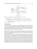
Adding the proposed approach to both protocols resulted in a different operation than the
original ones. Figure 11-A,B&C shows that, it is observed that S-MAC was improved over
SEA-MAC operation at low Duty-Cycle. This is due to the fact that S-MAC goes through
four stages of operation (SYNC+RTS+CST+ACK) while SEA-MAC has
(TONE+SYNC+RTS+CTS+ACK) which leads to a longer operation even with the
compression of two control packets (SYNC&RTS), SEA-MAC has longer operation time than
S-MAC at shorter duty-cycle.

98800
99000
99200
99400
99600
99800
100000
100200
0 1000 2000 3000 4000 5000 6000 7000

Time(s)
E n ergy(m J)
S-MAC-PP
SEA-MAC-PP

Fig. 11-A: PP+S-MAC vs. PP+SEA-MAC energy consumption at 5% Duty-Cycle.



0
0.5
1
1.5
2
2.5
3
3.5
0 1000 2000 3000 4000 5000 6000 7000
Time(s)
Avg. Message Delay(s)
S-MAC-PP
SEA-MAC-PP

Fig. 11-B: S-MAC-PP vs. SEA-MAC-PP average Delay at 5% Duty-Cycle.

0
10
20
30
40

50
60
0 1000 2000 3000 4000 5000 6000 7000
Time(s)
No. of collisions
S-MAC-PP
SEA-MAC-PP

Fig. 11-C: S-MAC-PP vs. SEA-MAC-PP collisions at 5% Duty-Cycles.

4.3 Pros and Cons of the proposed theory
Overall, the proposed approached satisfied the quest as it does improve the operation of
both protocols at different ranges of duty-cycle (we must note SEA-MAC with the proposed
approach offered better energy consumption and delay operation at higher duty-cycles than
S-MAC also implemented with the approach). Increasing the number of nodes result in
collision occurance rather than the situation with the straight line deployment. Overall
message delay is in favor of S-MAC at shorter duty-cycles and the advantage is to SEA-
MAC at longer duty-cycle.
In the next section we will discuss breifly the mobility issues in WSN as it is considered an
important part of this research area.

5. Mobility in WSN
Wireless sensor networks (WSN) offers a wide range of applications and it is also an intense
area of research. However, current research in wireless sensor networks focuses on
MAC & Mobility In Wireless Sensor Networks 291
0
20
40
60
80

100
120
0 1000 2000 3000 4000 5000 6000 7000
Time(s)
No. of collision
s
S-MAC
SEA-MAC

Fig. 10-C: S-MAC vs. SEA-MAC collisions ocurrances at 5% Duty-Cycle.

Adding the proposed approach to both protocols resulted in a different operation than the
original ones. Figure 11-A,B&C shows that, it is observed that S-MAC was improved over
SEA-MAC operation at low Duty-Cycle. This is due to the fact that S-MAC goes through
four stages of operation (SYNC+RTS+CST+ACK) while SEA-MAC has
(TONE+SYNC+RTS+CTS+ACK) which leads to a longer operation even with the
compression of two control packets (SYNC&RTS), SEA-MAC has longer operation time than
S-MAC at shorter duty-cycle.

98800
99000
99200
99400
99600
99800
100000
100200
0 1000 2000 3000 4000 5000 6000 7000
Time(s)
E n ergy(m J)

S-MAC-PP
SEA-MAC-PP

Fig. 11-A: PP+S-MAC vs. PP+SEA-MAC energy consumption at 5% Duty-Cycle.



0
0.5
1
1.5
2
2.5
3
3.5
0 1000 2000 3000 4000 5000 6000 7000
Time(s)
Avg. Message Delay(s)
S-MAC-PP
SEA-MAC-PP

Fig. 11-B: S-MAC-PP vs. SEA-MAC-PP average Delay at 5% Duty-Cycle.

0
10
20
30
40
50
60

0 1000 2000 3000 4000 5000 6000 7000
Time(s)
No. of collisions
S-MAC-PP
SEA-MAC-PP

Fig. 11-C: S-MAC-PP vs. SEA-MAC-PP collisions at 5% Duty-Cycles.

4.3 Pros and Cons of the proposed theory
Overall, the proposed approached satisfied the quest as it does improve the operation of
both protocols at different ranges of duty-cycle (we must note SEA-MAC with the proposed
approach offered better energy consumption and delay operation at higher duty-cycles than
S-MAC also implemented with the approach). Increasing the number of nodes result in
collision occurance rather than the situation with the straight line deployment. Overall
message delay is in favor of S-MAC at shorter duty-cycles and the advantage is to SEA-
MAC at longer duty-cycle.
In the next section we will discuss breifly the mobility issues in WSN as it is considered an
important part of this research area.

5. Mobility in WSN
Wireless sensor networks (WSN) offers a wide range of applications and it is also an intense
area of research. However, current research in wireless sensor networks focuses on
Wireless Sensor Networks: Application-Centric Design292
stationary WSN where they are deployed in a stationary position providing the base station
with information about the subject under observation. However, a mobile sensor network is
a collection of WSN nodes. Each of these nodes is capable of sensing, communication and
moving around. It is the mobility capabilities that distinguish a mobile sensor network from
the conventional ‘fixed’ WSN (Motari'c et al, 2002).
Mobile sensor networks offer many opportunities for research as these sensors involves: the
estimate location of the node in a movement scenario, an efficient DATA and information

processing schemes that can cope with the mobility measurements and requirements (this
includes the routing theory and the potential MAC Protocol Used).
Most of the discussed approaches interms of routing theory, MAC and also allocation the
location of the sensors are ment for stationary sensor nodes. Mobile sensor networks
requiers extra care when it comes to design and implementing a network related protocols
the conserns includes ad not exclusive to: energy consumption, message delay, location
estimation accuracy and scurity of information traveled between the nodes to the base
station.
To list some of the aspects that effects on designing an operapable Mobile sensor networks,
the next sections will give a brief explination about routing theory, MAC approaches and
Localaization scheme aimed for mobility applications.

5.1 Routing theory
Routing protocols are protocols aimed to offer transmitting the DATA through the network
by utilizing the best available routes (not always the shortest ones) to the destination. When
it comes to design routing protocols for mobile Sensor nodes, extra care should be taken in
terms of timing the transportation between the nodes. Most of the routing protocol that are
used and implemented for Wireless sensor networks (e.g. Ad hoc on demand Distance
Vector (AODV) and Dynamic Source Routing (DSR)) are originally designed and optimized
for ad hoc networks which utilizes devices like (Laptop computers and mobile phones)
which has much powerful energy sources than the ones available in sensor nodes. And to
the power issue mobility make the task even tougher.

5.2 MAC approaches
Even the approach discussed in this chapter does not satisfy the mobility issues in MAC
protocols aimed for mobile sensor networks. The results from the current work suggest that
the CSMA based MAC protocols has a better chance in overcoming this issue than TDMA
based MAC protocols because of the time slotting issues that comes along with TDMA
based systems. IEEE802.15.4 or best known as (Zigbee) is a MAC layer standard provided
by IEEE organization aimed for low power miniatures. Still, it cannot be considered yet as a

standard MAC protocols for mobile sensor networks as it is still in the development stages
for such applications.

5.3 Localization Issues
Locating the sensor is an important task in WSN as it provides information about the
phenomena monitored and what action should be taken at the occurrence of an action.
Proposed localization schemes are aimed manly for stationary networks and partially for
mobile networks. Some of the examples of localization techniques are (Boukerche et al,
2007):

RSSI: Received Signal Strength Indicator, which is the cheapest technique to establish a
node location as the medium used is wireless medium and most of the wireless adapter are
capable of capturing such information. The disadvantage of such approach is the accuracy
of the information calculated by such approach.

GPS: Geo- Positioning System, the most used approach mobile nodes application and in
some cases considered the easiest. The disadvantage of GPS systems is that it adds extra cost
to systems in terms of financial cost and energy consumption costs and also accuracy issues.

TOA: Time On Arrival systems, the most accurate approach to achieve the location of the
nodes. However there are some cons for this technique: first of all the cost is higher than
GPS systems. Second the accuracy issue is dependent on how violent the environment being
applied on as it requires a line-of-sight connection to capture the required information. And
the last issue, because it is a mounted platform so it will consume energy like the issue with
the GPS systems.

6. Future Research goals
The future research goal is to devise a template Network Model aimed for Mobile Wireless
Sensor Networks. The template will take in consideration the concerns discussed in section
five of this chapter. It is envisage that the proposed approach provided in this chapter can

assist to devise a MAC approach that can be applied for various applications in WSN. The
proposed template is designed for Habitat monitoring applications as they share some
similarities in terms of the configurations and crucial guarantees. Future work would to
utilize a Signal – to – noise Ratio estimator (Kamel, Jeoti, 2007) as a metric to define which
route is the best to chose and on which nodes signal can estimate the location of the node.
Cross-layer approach a definite approach and consideration that we aim utilize in our
template.

7. Acknowledgments
We are greateful to both Dr. Brahim Belhaouari Samir, department of Electrical and
Electronic Engineering in Universiti Teknologi PETRONAS, 31750 Tronoh, Perak for helping
us with proposed scheme mathmatical analysis. and Mr. Megual A. Erazo, Computer
science department in Florida international University for helping us to develop SEA-MAC
protocol. Our thanks goes also to Universiti Teknologi PETRONAS for funding this research
and achieve the aimed results.




MAC & Mobility In Wireless Sensor Networks 293
stationary WSN where they are deployed in a stationary position providing the base station
with information about the subject under observation. However, a mobile sensor network is
a collection of WSN nodes. Each of these nodes is capable of sensing, communication and
moving around. It is the mobility capabilities that distinguish a mobile sensor network from
the conventional ‘fixed’ WSN (Motari'c et al, 2002).
Mobile sensor networks offer many opportunities for research as these sensors involves: the
estimate location of the node in a movement scenario, an efficient DATA and information
processing schemes that can cope with the mobility measurements and requirements (this
includes the routing theory and the potential MAC Protocol Used).
Most of the discussed approaches interms of routing theory, MAC and also allocation the

location of the sensors are ment for stationary sensor nodes. Mobile sensor networks
requiers extra care when it comes to design and implementing a network related protocols
the conserns includes ad not exclusive to: energy consumption, message delay, location
estimation accuracy and scurity of information traveled between the nodes to the base
station.
To list some of the aspects that effects on designing an operapable Mobile sensor networks,
the next sections will give a brief explination about routing theory, MAC approaches and
Localaization scheme aimed for mobility applications.

5.1 Routing theory
Routing protocols are protocols aimed to offer transmitting the DATA through the network
by utilizing the best available routes (not always the shortest ones) to the destination. When
it comes to design routing protocols for mobile Sensor nodes, extra care should be taken in
terms of timing the transportation between the nodes. Most of the routing protocol that are
used and implemented for Wireless sensor networks (e.g. Ad hoc on demand Distance
Vector (AODV) and Dynamic Source Routing (DSR)) are originally designed and optimized
for ad hoc networks which utilizes devices like (Laptop computers and mobile phones)
which has much powerful energy sources than the ones available in sensor nodes. And to
the power issue mobility make the task even tougher.

5.2 MAC approaches
Even the approach discussed in this chapter does not satisfy the mobility issues in MAC
protocols aimed for mobile sensor networks. The results from the current work suggest that
the CSMA based MAC protocols has a better chance in overcoming this issue than TDMA
based MAC protocols because of the time slotting issues that comes along with TDMA
based systems. IEEE802.15.4 or best known as (Zigbee) is a MAC layer standard provided
by IEEE organization aimed for low power miniatures. Still, it cannot be considered yet as a
standard MAC protocols for mobile sensor networks as it is still in the development stages
for such applications.

5.3 Localization Issues
Locating the sensor is an important task in WSN as it provides information about the
phenomena monitored and what action should be taken at the occurrence of an action.
Proposed localization schemes are aimed manly for stationary networks and partially for
mobile networks. Some of the examples of localization techniques are (Boukerche et al,
2007):

RSSI: Received Signal Strength Indicator, which is the cheapest technique to establish a
node location as the medium used is wireless medium and most of the wireless adapter are
capable of capturing such information. The disadvantage of such approach is the accuracy
of the information calculated by such approach.

GPS: Geo- Positioning System, the most used approach mobile nodes application and in
some cases considered the easiest. The disadvantage of GPS systems is that it adds extra cost
to systems in terms of financial cost and energy consumption costs and also accuracy issues.

TOA: Time On Arrival systems, the most accurate approach to achieve the location of the
nodes. However there are some cons for this technique: first of all the cost is higher than
GPS systems. Second the accuracy issue is dependent on how violent the environment being
applied on as it requires a line-of-sight connection to capture the required information. And
the last issue, because it is a mounted platform so it will consume energy like the issue with
the GPS systems.

6. Future Research goals
The future research goal is to devise a template Network Model aimed for Mobile Wireless
Sensor Networks. The template will take in consideration the concerns discussed in section
five of this chapter. It is envisage that the proposed approach provided in this chapter can
assist to devise a MAC approach that can be applied for various applications in WSN. The
proposed template is designed for Habitat monitoring applications as they share some
similarities in terms of the configurations and crucial guarantees. Future work would to

utilize a Signal – to – noise Ratio estimator (Kamel, Jeoti, 2007) as a metric to define which
route is the best to chose and on which nodes signal can estimate the location of the node.
Cross-layer approach a definite approach and consideration that we aim utilize in our
template.

7. Acknowledgments
We are greateful to both Dr. Brahim Belhaouari Samir, department of Electrical and
Electronic Engineering in Universiti Teknologi PETRONAS, 31750 Tronoh, Perak for helping
us with proposed scheme mathmatical analysis. and Mr. Megual A. Erazo, Computer
science department in Florida international University for helping us to develop SEA-MAC
protocol. Our thanks goes also to Universiti Teknologi PETRONAS for funding this research
and achieve the aimed results.




Wireless Sensor Networks: Application-Centric Design294
8. References
Kazem Sohraby, Daniel Minoli and Taieb Znati “WIRELESS SENSOR NETWORKS
Technology, Protocols, and Applications”, 2007 by John Wiley & Sons, Inc.
Yang Yu, Viktor K Prasanna and Bhaskar Krishnamachari “Information processing and
routing in wireless sensor networks”, 2006 by World Scientific Publishing Co. Pte.
Ltd.
Bhaskar Krishnamachari “Networking Wireless Sensors”, Cambridge University Press 2005.
Alan Mainwaring, Joseph Polastre, Robert Szewczyk, David Culler and John Anderson
“Wireless Sensor Networks for Habitat Monitoring”,
WSNA’02, September 28, 2002,
Atlanta, Georgia, USA, ACM.
Vijay Raghunathan, Curt Schurgers, Sung Park, and Mani B. Srivastava “Energy Aware
Wireless Sensor Networks”, IEEE Signal Processing Magazine, 2002.

Azzedine Boukerche, Fernando H. S. Silva, Regina B. Araujo and Richard W. N. Pazzi “A
Low Latency and Energy Aware Event Ordering Algorithm for Wireless Actor and
Sensor Networks”, MSWiM’05,
October 10–13, 2005, Montreal, Quebec, Canada,
ACM.
Rebecca Braynard, Adam Silberstein and Carla Ellis “Extending Network Lifetime Using an
Automatically Tuned Energy-Aware MAC Protocol”, Proceedings of the 2006
European Workshop on Wireless Sensor Networks, Zurich, Switzerland (2006).
Lodewijk van Hoesel and Paul J.M. Havinga “MAC Protocol for WSNs”, SenSys'04,

November 3-5, 2004, Baltimore, Maryland, USA, ACM.
Yee Wei Law, Lodewijk van Hoesel, Jeroen Doumen, Pieter Hartel and Paul Havinga
“Energy Efficient Link Layer Jamming Attacks against Wireless Sensor Network
MAC Protocols”, SASN’05
, November 7, 2005, Alexandria, Virginia, USA, ACM.
Ioannis Mathioudakis, Neil M.White, Nick R. Harris, Geoff V. Merrett, “Wireless Sensor
Networks: A Case Study for Energy Efficient Environmental Monitoring”,
Eurosensors Conference 2008, 7-11 September 2008, Dresden, Germany.
Marwan Ihsan Shukur, Lee Sheng Chyan and Vooi Voon Yap “Wireless Sensor Networks:
Delay Guarentee and Energy Efficient MAC Protocols”, Proceedings of World
Academy of Science, Engineering and Technology, WCSET 2009, 25-27 Feb. 2009,
Penang, Malaysia.
Wei Ye, John Heidemann and Deborah Estrin “An Energy-Efficient MAC protocol for
Wireless Sensor Networks”, USC/ISI Technical Report ISI-TR-543, September 2001.
Tijs Van Dam and Keon Langendoen “An Adaptive Energy-Efficeint MAC Protocol for
Wireless Sensor Networks”, SenSys’03, November 5-7, 2003, ACM.
Shu Du, Amit Kumar Saha and David B. Johnson, “RMAC: A Routing-Enhanced Duty-
Cycle MAC Protocol for Wireless Sensor Networks”, INFOCOM 2007. 26th IEEE
International Conference on Computer Communications. IEEE.
Jin Kyung PARK, Woo Cheol Shin and Jun HA “Energy-Aware Pure ALOHA for Wireless

Sensor Networks”, IEIC Trans. Fundamentals, VOL.E89-A, No.6 June 2006.
Changsu Suh and Young-Bae Ko, “A Traffic Aware, Energy Efficient MAC protocol for
Wireless Sensor Networks”, Proceeding of the IEEE international symposium on
circuits and systems (IS CAS’05), May. 2005.
Sangheon Pack, Jaeyoung Choi, Taekyoung Kwon and Yanghee Choi, “TA-MAC: Task
Aware MAC Protocol for Wireless Sensor Networks”, Vehicular Technology
Conference, 2006. VTC 2006-Spring. IEEE 63rd.
Miguel A. Erazo, Yi Qian, “SEA-MAC: A Simple Energy Aware MAC Protocol for Wireless
Sensor Networks for Environmental Monitoring Applications”, Wireless Pervasive
Computing, 2007. ISWPC '07. IEEE 2
nd
international symposium 2007.
Rajgopal Kannan, Ram Kalidini and S. S. Iyengar “Energy and rate based MAC protocol for
Wireless Sensor Networks” SIGMOD Record, Vol.32, No.4, December 2003.
Anirudha Sahoo and Prashant Baronia “An Energy Efficient MAC in Wireless Sensor
Networks to Provide Delay Guarantee”, Local & Metropolitan Area Networks,
2007. LANMAN 2007. 15th IEEE Workshop on.
Saurabh Ganeriwal, Ram Kumar and Mani B. Srivastava “Timing-sync Protocol for Sensor
Networks”, SenSys ’03, November 5-7, 2003, Los Angeles, California, USA, ACM.
Esteban Egea-L´opez, Javier Vales-Alonso, Alejandro S. Mart´nez-Sala, Joan Garc´a-Haro,
Pablo Pav´on-Mari˜no, and M. Victoria Bueno-Delgado “A Real-Time MAC
Protocol for Wireless Sensor Networks: Virtual TDMA for Sensors (VTS)”, ARCS
2006, LNCS 3894, pp. 382–396, 2006, Springer-Verlag Berlin Heidelberg 2006.
Teerawat Issariyakul and Ekram Hossain “Introduction to Network Simulator NS2”,
SpringerLink publications-Springer US 2008.
Marwan Ihsan Shukur and Vooi Voon Yap “An Approach for efficient energy consumption
and delay guarantee MAC Protocol for Wireless Sensor Networks”, Proceedings of
International Conference on Computing and Informatics, ICOCI 2009, 24-25 June
2009, Kuala Lumpur, Malaysia, a.
Marwan Ihsan Shukur and Vooi Voon Yap “Enhanced SEA-MAC: An Efficient MAC

Protocol for Wireless Sensor Networks for Environmental Monitoring
Applications”, Conference on Innovative Technologies in Intelligent Systems and
Industrial Applications, IEEE CITISIA 2009, 25 July 2009, MONASH University
Sunway Campus, Malaysia, b.
Howard, A, Matari´c, M.J., and Sukhatme, G.S., “Mobile Sensor Network Deployment using
Potential Fields: A Distributed, Scalable Solution to the Area Coverage Problem”,
Proceedings of the 6th International Symposium on Distributed Autonomous Robotics
Systems (DARS02) Fukuoka, Japan, June 25-27, 2002.
Azzedine Boukerche, Horacio A. B. F. Oliveira and Eduardo F. Nakamura “Localization
Systems For Wireless Sensor Networks”, IEEE Wireless Communications Mag. Dec.
2007.
Nidal S. Kamel and Varun Jeoti “A Linear Prediction Based Estimation of Signal-to-Noise
Ratio in AWGN Channel”, ETRI journal, Volume 29, Number 5, October 2007.

MAC & Mobility In Wireless Sensor Networks 295
8. References
Kazem Sohraby, Daniel Minoli and Taieb Znati “WIRELESS SENSOR NETWORKS
Technology, Protocols, and Applications”, 2007 by John Wiley & Sons, Inc.
Yang Yu, Viktor K Prasanna and Bhaskar Krishnamachari “Information processing and
routing in wireless sensor networks”, 2006 by World Scientific Publishing Co. Pte.
Ltd.
Bhaskar Krishnamachari “Networking Wireless Sensors”, Cambridge University Press 2005.
Alan Mainwaring, Joseph Polastre, Robert Szewczyk, David Culler and John Anderson
“Wireless Sensor Networks for Habitat Monitoring”,
WSNA’02, September 28, 2002,
Atlanta, Georgia, USA, ACM.
Vijay Raghunathan, Curt Schurgers, Sung Park, and Mani B. Srivastava “Energy Aware
Wireless Sensor Networks”, IEEE Signal Processing Magazine, 2002.
Azzedine Boukerche, Fernando H. S. Silva, Regina B. Araujo and Richard W. N. Pazzi “A
Low Latency and Energy Aware Event Ordering Algorithm for Wireless Actor and

Sensor Networks”, MSWiM’05,
October 10–13, 2005, Montreal, Quebec, Canada,
ACM.
Rebecca Braynard, Adam Silberstein and Carla Ellis “Extending Network Lifetime Using an
Automatically Tuned Energy-Aware MAC Protocol”, Proceedings of the 2006
European Workshop on Wireless Sensor Networks, Zurich, Switzerland (2006).
Lodewijk van Hoesel and Paul J.M. Havinga “MAC Protocol for WSNs”, SenSys'04,

November 3-5, 2004, Baltimore, Maryland, USA, ACM.
Yee Wei Law, Lodewijk van Hoesel, Jeroen Doumen, Pieter Hartel and Paul Havinga
“Energy Efficient Link Layer Jamming Attacks against Wireless Sensor Network
MAC Protocols”, SASN’05
, November 7, 2005, Alexandria, Virginia, USA, ACM.
Ioannis Mathioudakis, Neil M.White, Nick R. Harris, Geoff V. Merrett, “Wireless Sensor
Networks: A Case Study for Energy Efficient Environmental Monitoring”,
Eurosensors Conference 2008, 7-11 September 2008, Dresden, Germany.
Marwan Ihsan Shukur, Lee Sheng Chyan and Vooi Voon Yap “Wireless Sensor Networks:
Delay Guarentee and Energy Efficient MAC Protocols”, Proceedings of World
Academy of Science, Engineering and Technology, WCSET 2009, 25-27 Feb. 2009,
Penang, Malaysia.
Wei Ye, John Heidemann and Deborah Estrin “An Energy-Efficient MAC protocol for
Wireless Sensor Networks”, USC/ISI Technical Report ISI-TR-543, September 2001.
Tijs Van Dam and Keon Langendoen “An Adaptive Energy-Efficeint MAC Protocol for
Wireless Sensor Networks”, SenSys’03, November 5-7, 2003, ACM.
Shu Du, Amit Kumar Saha and David B. Johnson, “RMAC: A Routing-Enhanced Duty-
Cycle MAC Protocol for Wireless Sensor Networks”, INFOCOM 2007. 26th IEEE
International Conference on Computer Communications. IEEE.
Jin Kyung PARK, Woo Cheol Shin and Jun HA “Energy-Aware Pure ALOHA for Wireless
Sensor Networks”, IEIC Trans. Fundamentals, VOL.E89-A, No.6 June 2006.
Changsu Suh and Young-Bae Ko, “A Traffic Aware, Energy Efficient MAC protocol for

Wireless Sensor Networks”, Proceeding of the IEEE international symposium on
circuits and systems (IS CAS’05), May. 2005.
Sangheon Pack, Jaeyoung Choi, Taekyoung Kwon and Yanghee Choi, “TA-MAC: Task
Aware MAC Protocol for Wireless Sensor Networks”, Vehicular Technology
Conference, 2006. VTC 2006-Spring. IEEE 63rd.
Miguel A. Erazo, Yi Qian, “SEA-MAC: A Simple Energy Aware MAC Protocol for Wireless
Sensor Networks for Environmental Monitoring Applications”, Wireless Pervasive
Computing, 2007. ISWPC '07. IEEE 2
nd
international symposium 2007.
Rajgopal Kannan, Ram Kalidini and S. S. Iyengar “Energy and rate based MAC protocol for
Wireless Sensor Networks” SIGMOD Record, Vol.32, No.4, December 2003.
Anirudha Sahoo and Prashant Baronia “An Energy Efficient MAC in Wireless Sensor
Networks to Provide Delay Guarantee”, Local & Metropolitan Area Networks,
2007. LANMAN 2007. 15th IEEE Workshop on.
Saurabh Ganeriwal, Ram Kumar and Mani B. Srivastava “Timing-sync Protocol for Sensor
Networks”, SenSys ’03, November 5-7, 2003, Los Angeles, California, USA, ACM.
Esteban Egea-L´opez, Javier Vales-Alonso, Alejandro S. Mart´nez-Sala, Joan Garc´a-Haro,
Pablo Pav´on-Mari˜no, and M. Victoria Bueno-Delgado “A Real-Time MAC
Protocol for Wireless Sensor Networks: Virtual TDMA for Sensors (VTS)”, ARCS
2006, LNCS 3894, pp. 382–396, 2006, Springer-Verlag Berlin Heidelberg 2006.
Teerawat Issariyakul and Ekram Hossain “Introduction to Network Simulator NS2”,
SpringerLink publications-Springer US 2008.
Marwan Ihsan Shukur and Vooi Voon Yap “An Approach for efficient energy consumption
and delay guarantee MAC Protocol for Wireless Sensor Networks”, Proceedings of
International Conference on Computing and Informatics, ICOCI 2009, 24-25 June
2009, Kuala Lumpur, Malaysia, a.
Marwan Ihsan Shukur and Vooi Voon Yap “Enhanced SEA-MAC: An Efficient MAC
Protocol for Wireless Sensor Networks for Environmental Monitoring
Applications”, Conference on Innovative Technologies in Intelligent Systems and

Industrial Applications, IEEE CITISIA 2009, 25 July 2009, MONASH University
Sunway Campus, Malaysia, b.
Howard, A, Matari´c, M.J., and Sukhatme, G.S., “Mobile Sensor Network Deployment using
Potential Fields: A Distributed, Scalable Solution to the Area Coverage Problem”,
Proceedings of the 6th International Symposium on Distributed Autonomous Robotics
Systems (DARS02) Fukuoka, Japan, June 25-27, 2002.
Azzedine Boukerche, Horacio A. B. F. Oliveira and Eduardo F. Nakamura “Localization
Systems For Wireless Sensor Networks”, IEEE Wireless Communications Mag. Dec.
2007.
Nidal S. Kamel and Varun Jeoti “A Linear Prediction Based Estimation of Signal-to-Noise
Ratio in AWGN Channel”, ETRI journal, Volume 29, Number 5, October 2007.


X

Hybrid Optical and Wireless Sensor Networks

Lianshan Yan, Xiaoyin Li, Zhen Zhang, Jiangtao Liu and Wei Pan
Southwest Jiaotong University
Chengdu, Sichuan, China

1. Introduction
Wireless sensor network (WSN) has attracted considerable attentions during the last few
years due to characteristics such as feasibility of rapid deployment, self-organization
(different from ad hoc networks though) and fault tolerance, as well as rapid development
of wireless communications and integrated electronics [1]. Such networks are constructed by
randomly but densely scattered tiny sensor nodes (Fig. 1). As sensor nodes are prone to
failures and the network topology changes very frequently, different protocols have been
proposed to save the overall energy dissipation in WSNs [2-5]. Among them, Low-Energy-
Adaptive-Clustering-Hierarchy (LEACH), first proposed by researchers from Massachusetts

Institute of Technology [5], is considered to be one of the most effective protocols in terms of
energy efficiency [6-7]. Another protocol, called Power-Efficient Gathering in Sensor
Information Systems (PEGASIS), is a near optimal chain-based protocol [8].

WSN
WSN Nodes
SINK
WSN
WSN Nodes
SINK

Fig. 1. Illustration of a wireless sensor network (WSN) with randomly scattered nodes (sink
node: no energy restriction; WSN nodes: with energy restriction);

On the other hand, distributed fiber sensors (DFS) have been intensively studied or even
deployed for analyzing loss, external pressure and temperature or birefringence distribution
along the fiber link, ranging from hundreds of meters to tens of kilometers [9-13].
Mechanisms include Rayleigh, Brillouin or Raman scattering or polarization effects, through
either time or frequency-domain analysis. Compared with conventional sensors including
Hybrid Optical and Wireless Sensor Networks 297
Hybrid Optical and Wireless Sensor Networks
Lianshan Yan, Xiaoyin Li, Zhen Zhang, Jiangtao Liu and Wei Pan
16

wireless ones, optical fiber sensors have intrinsic advantages such as high sensitivity, the
immunity to electromagnetic interference (EMI), superior endurance in harsh environments
and much longer lifetime.
Apparently it would be highly desirable to have integrated sensor networks that can take
advantages of both WSNs and fiber sensor networks (FSNs). Such hybrid sensor networks
can find major applications including monitoring inaccessible terrains (military, high-

voltage electricity facilities, etc.), long-term observation of earthquake activity and large area
environmental control with tunnels, and so on. So far hybrid sensor networks have been
studied as well [14-16], while optical sensors in these networks are generally point-like (e.g.
fiber-Bragg-grating based), and such nodes can be regarded as normal WSN nodes after
optical to wireless signal conversion.
In this chapter, we first review typical WSN protocols, mainly about LEACH and PEGASIS,
then evaluate the performance of LEACH protocols for different topologies, especially the
rectangle one. We propose an improved algorithm based on LEACH and PEGASIS for the
WSN, finally and most importantly, we propose an O-LEACH protocol for the hybrid
sensor network that is composed of a DFS link and two separated WSNs. Most analyses
about performance are done in terms of lifetime of the sensor networks.

2. Overview of WSN protocols
Wireless sensor networks (WSNs) generally are composed of small or tiny nodes with
sensing, computation, and communication capabilities. Various routing, power
management, and data dissemination protocols have been specifically designed for WSNs
where energy awareness is an essential design issue. Among them, routing protocols might
differ depending on the applications and network architectures. In general, routing
protocols for the wireless sensor networks can be divided into flat-based, hierarchical-based,
and location-based in terms of the underlying network structures [17-19]. As some protocols
may be discussed intensively in other chapters of this book, here we give a brief review
about major protocols.
(1) Flat-based routing protocol
Sensor nodes in flat-based routing protocols have the same role and collaborate together to
perform the sensing task and multi-hop communication. Since the flat routing is based on
flooding, it has several demerits, such as large routing overhead and high energy
dissipation. Flat-based routing protocol is used in the early stage of WSNs, such as Flooding,
Gossiping, SPIN, and Rumor.
(2) Hierarchical-based routing protocol
Hierarchical-based routing protocol is the main trend for WSN’s routing protocols. In

hierarchical-based routing protocols, the network is divided into several logical groups
within a fixed area. The logical groups are called clusters. Sensor nodes collect the
information in a cluster and a head node aggregates the information. Each sensor node
delivers the sensing data to the head node in the cluster and the head node delivers the
aggregated data to the base station which is located outside of the sensor network. Contrary
to flat routing protocols, only a head node aggregates the collected information and sends it
to the base station. Due to these advantages, sensor nodes can remarkably save their own
s

energy. In general, a hierarchical routing technique is regarded as superior to flat routing
approaches. The classical Hierarchical-based routing protocols are LEACH, PEGASIS, H-
PEGASIS, TEEN, and APTEEN. We will discuss the LEACH and PEGASIS protocols in
more details later.
(3) Location-based routing protocol
Such protocol is based on the location information of senor nodes in WSNs. It assumes that
each node would know its own location and its neighbor sensor nodes’ location before
sensor nodes sensing and collecting the peripheral information. The distance between
neighbouring sensor nodes can be computed based on the incoming signal strength [17-18].

2.1 LEACH
Low Energy Adaptive Clustering Hierarchy (LEACH) was first introduced by Heinzelman,
et al. in [5, 20] with advantages such as energy efficiency, simplicity and load balancing
ability. LEACH is a cluster-based protocol, therefore the numbers of cluster heads and
cluster members generated by LEACH are important parameters for achieving better
performance.
In LEACH protocol, the sensor nodes in the network are divided into a number of clusters,
the nodes organize themselves into preferred local clusters, a sensor node is selected
randomly as the cluster head (CH) in each cluster and this role is rotated to evenly distribute
the energy load among nodes of the network. The CH nodes compress data arriving from
nodes that belong to the respective cluster, and send an aggregated packet to the BS in order

to further reduce the amount of information that must be transmitted to the BS, thus
reducing energy dissipation and enhancing system lifetime. After a given interval of time,
randomized rotation of the role of CH is conducted to maximize the uniformity of energy
dissipation of the network. Sensors elect themselves to be local cluster heads at any time
with a certain probability. Generally only ~ 5% of nodes need to act as CHs based on
simulation results. LEACH uses a TDMA/CDMA MAC to reduce intercluster and
intracluster collisions. As data collection is centralized and performed periodically, this
protocol is most appropriate when there is a need for constant monitoring by the sensor
network.
The operation of LEACH is broken up into rounds, where each round begins with a set-up
phase followed by a steady-state phase. In order to minimize overhead, the steady-state
phase takes longer time compared to the set-up phase. In the setup phase, the clusters are
organized and CHs are selected. In the steady state phase, the actual data transfer to the BS
takes place. During the setup phase, each node decides whether or not to become a cluster
head for the current round. A predetermined fraction of nodes, p, elect themselves as CHs.
A sensor node chooses a random number between 0 and 1. If this random number is less
than a threshold value T(n), , the node becomes a cluster head for the current round. The
threshold value is calculated based on Eq. (2-1):


1
1 *( mod )
( )
0
p
if n G
p r
T n
p
otherwise











(2-1)

Wireless Sensor Networks: Application-Centric Design298

wireless ones, optical fiber sensors have intrinsic advantages such as high sensitivity, the
immunity to electromagnetic interference (EMI), superior endurance in harsh environments
and much longer lifetime.
Apparently it would be highly desirable to have integrated sensor networks that can take
advantages of both WSNs and fiber sensor networks (FSNs). Such hybrid sensor networks
can find major applications including monitoring inaccessible terrains (military, high-
voltage electricity facilities, etc.), long-term observation of earthquake activity and large area
environmental control with tunnels, and so on. So far hybrid sensor networks have been
studied as well [14-16], while optical sensors in these networks are generally point-like (e.g.
fiber-Bragg-grating based), and such nodes can be regarded as normal WSN nodes after
optical to wireless signal conversion.
In this chapter, we first review typical WSN protocols, mainly about LEACH and PEGASIS,
then evaluate the performance of LEACH protocols for different topologies, especially the
rectangle one. We propose an improved algorithm based on LEACH and PEGASIS for the
WSN, finally and most importantly, we propose an O-LEACH protocol for the hybrid
sensor network that is composed of a DFS link and two separated WSNs. Most analyses

about performance are done in terms of lifetime of the sensor networks.

2. Overview of WSN protocols
Wireless sensor networks (WSNs) generally are composed of small or tiny nodes with
sensing, computation, and communication capabilities. Various routing, power
management, and data dissemination protocols have been specifically designed for WSNs
where energy awareness is an essential design issue. Among them, routing protocols might
differ depending on the applications and network architectures. In general, routing
protocols for the wireless sensor networks can be divided into flat-based, hierarchical-based,
and location-based in terms of the underlying network structures [17-19]. As some protocols
may be discussed intensively in other chapters of this book, here we give a brief review
about major protocols.
(1) Flat-based routing protocol
Sensor nodes in flat-based routing protocols have the same role and collaborate together to
perform the sensing task and multi-hop communication. Since the flat routing is based on
flooding, it has several demerits, such as large routing overhead and high energy
dissipation. Flat-based routing protocol is used in the early stage of WSNs, such as Flooding,
Gossiping, SPIN, and Rumor.
(2) Hierarchical-based routing protocol
Hierarchical-based routing protocol is the main trend for WSN’s routing protocols. In
hierarchical-based routing protocols, the network is divided into several logical groups
within a fixed area. The logical groups are called clusters. Sensor nodes collect the
information in a cluster and a head node aggregates the information. Each sensor node
delivers the sensing data to the head node in the cluster and the head node delivers the
aggregated data to the base station which is located outside of the sensor network. Contrary
to flat routing protocols, only a head node aggregates the collected information and sends it
to the base station. Due to these advantages, sensor nodes can remarkably save their own
s

energy. In general, a hierarchical routing technique is regarded as superior to flat routing

approaches. The classical Hierarchical-based routing protocols are LEACH, PEGASIS, H-
PEGASIS, TEEN, and APTEEN. We will discuss the LEACH and PEGASIS protocols in
more details later.
(3) Location-based routing protocol
Such protocol is based on the location information of senor nodes in WSNs. It assumes that
each node would know its own location and its neighbor sensor nodes’ location before
sensor nodes sensing and collecting the peripheral information. The distance between
neighbouring sensor nodes can be computed based on the incoming signal strength [17-18].

2.1 LEACH
Low Energy Adaptive Clustering Hierarchy (LEACH) was first introduced by Heinzelman,
et al. in [5, 20] with advantages such as energy efficiency, simplicity and load balancing
ability. LEACH is a cluster-based protocol, therefore the numbers of cluster heads and
cluster members generated by LEACH are important parameters for achieving better
performance.
In LEACH protocol, the sensor nodes in the network are divided into a number of clusters,
the nodes organize themselves into preferred local clusters, a sensor node is selected
randomly as the cluster head (CH) in each cluster and this role is rotated to evenly distribute
the energy load among nodes of the network. The CH nodes compress data arriving from
nodes that belong to the respective cluster, and send an aggregated packet to the BS in order
to further reduce the amount of information that must be transmitted to the BS, thus
reducing energy dissipation and enhancing system lifetime. After a given interval of time,
randomized rotation of the role of CH is conducted to maximize the uniformity of energy
dissipation of the network. Sensors elect themselves to be local cluster heads at any time
with a certain probability. Generally only ~ 5% of nodes need to act as CHs based on
simulation results. LEACH uses a TDMA/CDMA MAC to reduce intercluster and
intracluster collisions. As data collection is centralized and performed periodically, this
protocol is most appropriate when there is a need for constant monitoring by the sensor
network.
The operation of LEACH is broken up into rounds, where each round begins with a set-up

phase followed by a steady-state phase. In order to minimize overhead, the steady-state
phase takes longer time compared to the set-up phase. In the setup phase, the clusters are
organized and CHs are selected. In the steady state phase, the actual data transfer to the BS
takes place. During the setup phase, each node decides whether or not to become a cluster
head for the current round. A predetermined fraction of nodes, p, elect themselves as CHs.
A sensor node chooses a random number between 0 and 1. If this random number is less
than a threshold value T(n), , the node becomes a cluster head for the current round. The
threshold value is calculated based on Eq. (2-1):


1
1 *( mod )
( )
0
p
if n G
p r
T n
p
otherwise











(2-1)

Hybrid Optical and Wireless Sensor Networks 299

Where p is the desired percentage of the cluster heads (e.g. p=0.05), r is the current round,
and G is the set of nodes that have not been cluster heads in the last 1/p rounds. Using this
threshold, each node may be a cluster head sometime within 1/p rounds. All elected CHs
broadcast an advertisement message to the rest of nodes in the network that they are the
new CHs. After receiving the advertisement, all non-CH nodes decide on the cluster to
which they want to belong based on the signal strength of the advertisement. The non-CH
nodes then inform the appropriate CHs to be a member of the cluster. After receiving all the
messages from the nodes that would like to be included in the cluster and based on the
number of nodes in the cluster, the CH node creates a TDMA schedule and assigns each
node a time slot when it can transmit information. This schedule is broadcast to all the
nodes in the cluster. During the steady state phase, the sensor nodes can begin sensing and
transmitting data to the CHs. The CH node must keep its receiver on to receive all the data
from the nodes in the cluster. Each cluster communicates using different CDMA codes to
reduce interference from nodes belonging to other clusters. After receiving all the data, the
CH aggregates the data before sending it to the BS. This ends a typical round.
Advantages of LEACH include: (i) by using adaptive clusters and rotating cluster heads,
LEACH allows the energy requirements of the system to be distributed among all the
sensors; (ii) LEACH is able to perform local computation in each cluster to reduce the
amount of data that must be transmitted to the base station. On the other hand, there are
still some drawbacks about LEACH: (i) LEACH assumes that each node could communicate
with the sink and each node has computational power to support different MAC protocols,
which limits its application to networks deployed in large regions. (ii) LEACH does not
determine how to distribute the CHs uniformly through the network. Therefore, there is the
possibility that the elected CHs will be concentrated in one part of the network. (iii) LEACH
assumes that all nodes begin with the same amount of energy capacity in each election
round, assuming that being a CH consumes approximately the same amount of energy for

each node. Hence LEACH is not appropriate for non-uniform energy nodes [17, 20].

2.2 PEGASIS
In [8], an enhancement over the LEACH protocol called Power-Efficient Gathering in Sensor
Information Systems (PEGASIS) was proposed. The basic idea of the protocol is that nodes
only receive from and transmit to the closest neighbours, and they take turns being the
leader for communicating with the BS. This reduces the power required to transmit data per
round as the power draining is spread uniformly over all nodes. Hence, PEGASIS has two
main objectives: (i) to increase the lifetime of each node by using collaborative techniques; (ii)
to allow only local coordination between nodes that are close together so that the bandwidth
consumed in communication is reduced.
PEGASIS adopts a homogenous topology. In this topology, the BS lies far from sensors with
the fixed position. The data is collected and compressed before sent to the next node. Hence
the messages maintain ideally a fixed size when they are transmitted between sensors. To
locate the closest neighbour node in PEGASIS, each node uses the signal strength to
measure the distance to all neighbouring nodes and then adjusts the signal strength so that
only one node can be heard. The chain in PEGASIS consists of those nodes that are closest to
each other and form a path to the BS. The following describes the protocol briefly:
s

1) The chain starts with the furthest node from the BS to make sure that nodes father
from the BS have close neighbours. Based on the greedy algorithm, the neighbour
node joins into the chain with its distance increases gradually. When a node dies, the
chain is reconstructed in the same manner to bypass the dead node.
2) To gather data in each round, a token is generated by the BS to set the aggregating
direction after the token sent from the BS to an end node. Each node receives data
from one neighbour, fuses with its own data, and transmits to the other neighbour on
the chain.
3) Only one node transmits data to the BS in certain rounds, the leader is the node
whose number is (i mod N) where N represents the number of the nodes in round i.

PEGASIS is better than LEACH in terms of energy saving due to following facts: (i) During
the data localization, the distances that most of the nodes transmit information are much
shorter compared to that in LEACH. (ii) The amount of data for the leader to receive is much
less than LEACH. (iii) only one node transmits to the BS in each round.
Though PEGASIS has obvious advantages, it has some shortcomings. Firstly, though most
sensors are joined on a chain to form a basically homogenous structure, a sensor with too
much branches may perform many times of data receiving in a certain round thereby
resulting in unbalanced energy problem. Secondly, all the nodes must keep active before the
token arriving. This means there will be a large percentage of active nodes with nothing to
do from the beginning, meaning a waste of energy and time. Thirdly, once a sensor on the
chain was captured the whole net may be under the control by the attackers. The weak
security could be a great threat [17, 20].
LEACH that is a cluster-based protocol and PEGASIS that is a chain-based protocol are the
most classical Hierarchical-based routing protocols. They both have attracted intensive
attention, and lots of routing protocols are based on these two. Next we will investigate
some issues in details.

3. WSN Topologies
3.1 Shapes of different topologies
According to the shape of WSN monitoring area, application requirements and monitoring
of different targets, different topologies should be chosen for deploying the WSN: circular
topology is preferred for applications such as harbour, stadium etc. [21]; square topology is
suitable for irrigation in agriculture, nature reserve area etc.; rectangular topology can be
chosen for highway, railway, mine and other areas [22].
Here we study the life time of WSN in round, square, rectangular shapes of topology, and
the three topologies are shown in Figs. 3.1 (a-c). In Fig. 3.1(a), the circular area is 10,000m
2

(same as square, rectangular areas) with the radius R= 56.419m and the base station is
located at the center of the circle, i.e. (0, 0). In Fig. 3.1(b), the size of the square area is

100x100m
2
with the base station located on (0, 50) or (50, 175). In Fig.3.1(c), the size of the
rectangular area is 50*200m with the base station located on (0, 25) or (100, 150).

Wireless Sensor Networks: Application-Centric Design300

Where p is the desired percentage of the cluster heads (e.g. p=0.05), r is the current round,
and G is the set of nodes that have not been cluster heads in the last 1/p rounds. Using this
threshold, each node may be a cluster head sometime within 1/p rounds. All elected CHs
broadcast an advertisement message to the rest of nodes in the network that they are the
new CHs. After receiving the advertisement, all non-CH nodes decide on the cluster to
which they want to belong based on the signal strength of the advertisement. The non-CH
nodes then inform the appropriate CHs to be a member of the cluster. After receiving all the
messages from the nodes that would like to be included in the cluster and based on the
number of nodes in the cluster, the CH node creates a TDMA schedule and assigns each
node a time slot when it can transmit information. This schedule is broadcast to all the
nodes in the cluster. During the steady state phase, the sensor nodes can begin sensing and
transmitting data to the CHs. The CH node must keep its receiver on to receive all the data
from the nodes in the cluster. Each cluster communicates using different CDMA codes to
reduce interference from nodes belonging to other clusters. After receiving all the data, the
CH aggregates the data before sending it to the BS. This ends a typical round.
Advantages of LEACH include: (i) by using adaptive clusters and rotating cluster heads,
LEACH allows the energy requirements of the system to be distributed among all the
sensors; (ii) LEACH is able to perform local computation in each cluster to reduce the
amount of data that must be transmitted to the base station. On the other hand, there are
still some drawbacks about LEACH: (i) LEACH assumes that each node could communicate
with the sink and each node has computational power to support different MAC protocols,
which limits its application to networks deployed in large regions. (ii) LEACH does not
determine how to distribute the CHs uniformly through the network. Therefore, there is the

possibility that the elected CHs will be concentrated in one part of the network. (iii) LEACH
assumes that all nodes begin with the same amount of energy capacity in each election
round, assuming that being a CH consumes approximately the same amount of energy for
each node. Hence LEACH is not appropriate for non-uniform energy nodes [17, 20].

2.2 PEGASIS
In [8], an enhancement over the LEACH protocol called Power-Efficient Gathering in Sensor
Information Systems (PEGASIS) was proposed. The basic idea of the protocol is that nodes
only receive from and transmit to the closest neighbours, and they take turns being the
leader for communicating with the BS. This reduces the power required to transmit data per
round as the power draining is spread uniformly over all nodes. Hence, PEGASIS has two
main objectives: (i) to increase the lifetime of each node by using collaborative techniques; (ii)
to allow only local coordination between nodes that are close together so that the bandwidth
consumed in communication is reduced.
PEGASIS adopts a homogenous topology. In this topology, the BS lies far from sensors with
the fixed position. The data is collected and compressed before sent to the next node. Hence
the messages maintain ideally a fixed size when they are transmitted between sensors. To
locate the closest neighbour node in PEGASIS, each node uses the signal strength to
measure the distance to all neighbouring nodes and then adjusts the signal strength so that
only one node can be heard. The chain in PEGASIS consists of those nodes that are closest to
each other and form a path to the BS. The following describes the protocol briefly:
s

1) The chain starts with the furthest node from the BS to make sure that nodes father
from the BS have close neighbours. Based on the greedy algorithm, the neighbour
node joins into the chain with its distance increases gradually. When a node dies, the
chain is reconstructed in the same manner to bypass the dead node.
2) To gather data in each round, a token is generated by the BS to set the aggregating
direction after the token sent from the BS to an end node. Each node receives data
from one neighbour, fuses with its own data, and transmits to the other neighbour on

the chain.
3) Only one node transmits data to the BS in certain rounds, the leader is the node
whose number is (i mod N) where N represents the number of the nodes in round i.
PEGASIS is better than LEACH in terms of energy saving due to following facts: (i) During
the data localization, the distances that most of the nodes transmit information are much
shorter compared to that in LEACH. (ii) The amount of data for the leader to receive is much
less than LEACH. (iii) only one node transmits to the BS in each round.
Though PEGASIS has obvious advantages, it has some shortcomings. Firstly, though most
sensors are joined on a chain to form a basically homogenous structure, a sensor with too
much branches may perform many times of data receiving in a certain round thereby
resulting in unbalanced energy problem. Secondly, all the nodes must keep active before the
token arriving. This means there will be a large percentage of active nodes with nothing to
do from the beginning, meaning a waste of energy and time. Thirdly, once a sensor on the
chain was captured the whole net may be under the control by the attackers. The weak
security could be a great threat [17, 20].
LEACH that is a cluster-based protocol and PEGASIS that is a chain-based protocol are the
most classical Hierarchical-based routing protocols. They both have attracted intensive
attention, and lots of routing protocols are based on these two. Next we will investigate
some issues in details.

3. WSN Topologies
3.1 Shapes of different topologies
According to the shape of WSN monitoring area, application requirements and monitoring
of different targets, different topologies should be chosen for deploying the WSN: circular
topology is preferred for applications such as harbour, stadium etc. [21]; square topology is
suitable for irrigation in agriculture, nature reserve area etc.; rectangular topology can be
chosen for highway, railway, mine and other areas [22].
Here we study the life time of WSN in round, square, rectangular shapes of topology, and
the three topologies are shown in Figs. 3.1 (a-c). In Fig. 3.1(a), the circular area is 10,000m
2

(same as square, rectangular areas) with the radius R= 56.419m and the base station is
located at the center of the circle, i.e. (0, 0). In Fig. 3.1(b), the size of the square area is
100x100m
2
with the base station located on (0, 50) or (50, 175). In Fig.3.1(c), the size of the
rectangular area is 50*200m with the base station located on (0, 25) or (100, 150).

Hybrid Optical and Wireless Sensor Networks 301

-60 -30 0 30 60
-60
-30
0
30
60
m
m

0 25 50 75 100
0
25
50
75
100
m
m

(a) Circular topology (b) Square topology

0 50 100 150 200
0
25
50
m
m
Zone 1
Zone 2
Zone 3
Zone 4

(c) Rectangle topology
Fig 3.1 Three different types of WSN’s topology:
Sink (a):(0,0); (b):(0,50) or (50,175); (c):(0,25) or (100,150)

The probability of cluster head node in the LEACH protocol has a certain impact on the
WSN’s lifetime. In our analysis, we divides the rectangle area into four smaller square areas,
with the communication distance of nodes keeping short (d
B
<d
0
, where d
B
is the
broadcasting distance of the cluster head). From the first-order radio model, we can get the
optimal cluster head probability formula as follows:

2
opt
toBS

N M
k
d

 
(3-1)

Where N is the number of sensor nodes. In the rectangular region 100 nodes are scattered
randomly, and the region is divided into four regions. In order to verify the difference of the
number of nodes distributed in different regions, we simulate 100 independent iterations of
the nodes’ number in each region, and get the averages in the four regions as zone1(25.32)、
zone2(24.83)、zone3(24.87) and zone4(24.98). It can be seen that the number of nodes in
each region are around 25, there’re almost no difference in the average nodes’ numbers for
the four regions, so in the text, the nodes are uniform distributed in the four regions, i.e.
N=25. M is the side length of each small square region, here M=50. d
toBS
is the distance
between the sink and the node. As the distance of a node to the base station is different, we
can change the percentage of cluster heads in different regions to reach the optimal value so
that the lifetime of the whole WSN can be prolonged.
For the topology with a rectangular shape, we propose an improved LEACH algorithm. The
main idea is described as follows:
s

(1) Divide the rectangular area into several small square areas with the same size;
(2) Elect the cluster heads separately in each region, and the optimal probabilities of the
cluster heads for each region can be obtained from Eq. (3-1), i.e. the values are
p
1
=0.02，p

2
=0.03, p
3
=0.03, p
4
=0.02；
(3) After the cluster heads in each region are selected, the rest of the protocol is similar
to LEACH.
The improved algorithm elects cluster heads in each region according to its probability of
the cluster heads. In this way, it can make sure that there are clusters in every region and
ensure the clusters distributed more uniformly in every region, which reduces the energy
dissipation and improves the lifetime of the network.

3.2 Simulation results
We simulate the three shapes of topology that use (improved) LEACH as the routing
protocol. Parameters used in simulation are listed in table 3.1. There are 100 sensor nodes
randomly scattered with fixed position in each shape. We measure the round number when
the first node died, 20% of nodes died and 50% of nodes died respectively as the criterion to
estimate the lifetime of WSN.

Parameter Value
Number of nodes 100
Initial energy (J) 0.5
Data packet length (bit) 4000
Control packet length(bit) 200
Energy dissipation of one Tx (nJ) 50
Energy dissipation of one Rx (nJ) 50
Energy aggregation energy (nJ) 5
Energy loss-free space (pJ/bit/m
2

) 10
Energy loss-multipass fading (pJ/bit/m
4
) 0.0013
Table 3.1 Parameters used in simulation

Table 3.2 shows the round numbers (the lifetime) of WSN for different BS locations and
different percentage of dead nodes in circle, square and rectangular shapes of topology. As
the sensor nodes distributed randomly in WSN that may statistically vary, we simulate
every case for 100 iterations to get more accurate results. The percentage of the cluster heads
is set to 5% in three shapes of topology. It can be seen from Table 3.2 that the longest lifetime
of WSN is the circle shape of topology. The BS located in the center of the circle that is
symmetric, so that the energy dissipation of nodes are more even and the lifetime of the
network is prolonged. For the rectangle shape, the lifetime is different as the position of BS
changes. Simulation results indicate that the lifetime for the BS in (0, 50) is longer that in
(50,175). As the BS in (0, 50) is nearer to the sensor area, the energy for transmitting data to
the BS is reduced.


Wireless Sensor Networks: Application-Centric Design302

-60 -30 0 30 60
-60
-30
0
30
60
m
m

0 25 50 75 100
0
25
50
75
100
m
m

(a) Circular topology (b) Square topology

0 50 100 150 200
0
25
50
m
m
Zone 1
Zone 2
Zone 3
Zone 4

(c) Rectangle topology
Fig 3.1 Three different types of WSN’s topology:
Sink (a):(0,0); (b):(0,50) or (50,175); (c):(0,25) or (100,150)

The probability of cluster head node in the LEACH protocol has a certain impact on the
WSN’s lifetime. In our analysis, we divides the rectangle area into four smaller square areas,
with the communication distance of nodes keeping short (d
B

<d
0
, where d
B
is the
broadcasting distance of the cluster head). From the first-order radio model, we can get the
optimal cluster head probability formula as follows:

2
opt
toBS
N M
k
d

 
(3-1)

Where N is the number of sensor nodes. In the rectangular region 100 nodes are scattered
randomly, and the region is divided into four regions. In order to verify the difference of the
number of nodes distributed in different regions, we simulate 100 independent iterations of
the nodes’ number in each region, and get the averages in the four regions as zone1(25.32)、
zone2(24.83)、zone3(24.87) and zone4(24.98). It can be seen that the number of nodes in
each region are around 25, there’re almost no difference in the average nodes’ numbers for
the four regions, so in the text, the nodes are uniform distributed in the four regions, i.e.
N=25. M is the side length of each small square region, here M=50. d
toBS
is the distance
between the sink and the node. As the distance of a node to the base station is different, we
can change the percentage of cluster heads in different regions to reach the optimal value so

that the lifetime of the whole WSN can be prolonged.
For the topology with a rectangular shape, we propose an improved LEACH algorithm. The
main idea is described as follows:
s

(1) Divide the rectangular area into several small square areas with the same size;
(2) Elect the cluster heads separately in each region, and the optimal probabilities of the
cluster heads for each region can be obtained from Eq. (3-1), i.e. the values are
p
1
=0.02，p
2
=0.03, p
3
=0.03, p
4
=0.02；
(3) After the cluster heads in each region are selected, the rest of the protocol is similar
to LEACH.
The improved algorithm elects cluster heads in each region according to its probability of
the cluster heads. In this way, it can make sure that there are clusters in every region and
ensure the clusters distributed more uniformly in every region, which reduces the energy
dissipation and improves the lifetime of the network.

3.2 Simulation results
We simulate the three shapes of topology that use (improved) LEACH as the routing
protocol. Parameters used in simulation are listed in table 3.1. There are 100 sensor nodes
randomly scattered with fixed position in each shape. We measure the round number when
the first node died, 20% of nodes died and 50% of nodes died respectively as the criterion to
estimate the lifetime of WSN.

Parameter Value
Number of nodes 100
Initial energy (J) 0.5
Data packet length (bit) 4000
Control packet length(bit) 200
Energy dissipation of one Tx (nJ) 50
Energy dissipation of one Rx (nJ) 50
Energy aggregation energy (nJ) 5
Energy loss-free space (pJ/bit/m
2
) 10
Energy loss-multipass fading (pJ/bit/m
4
) 0.0013
Table 3.1 Parameters used in simulation

Table 3.2 shows the round numbers (the lifetime) of WSN for different BS locations and
different percentage of dead nodes in circle, square and rectangular shapes of topology. As
the sensor nodes distributed randomly in WSN that may statistically vary, we simulate
every case for 100 iterations to get more accurate results. The percentage of the cluster heads
is set to 5% in three shapes of topology. It can be seen from Table 3.2 that the longest lifetime
of WSN is the circle shape of topology. The BS located in the center of the circle that is
symmetric, so that the energy dissipation of nodes are more even and the lifetime of the
network is prolonged. For the rectangle shape, the lifetime is different as the position of BS
changes. Simulation results indicate that the lifetime for the BS in (0, 50) is longer that in
(50,175). As the BS in (0, 50) is nearer to the sensor area, the energy for transmitting data to
the BS is reduced.

Hybrid Optical and Wireless Sensor Networks 303

Topology

Circle Square Rectangle
Sink (0, 0) (0,50)

(50, 175)

(0, 25)

(100,150)
1% 757 740 639 470 555
20% 854 846 715 644 652
50% 923 919 788 785 717
Table 3.2 Lifetime comparisons of different shapes of topology

It can be seen form Table 3.2 that the lifetimes of the rectangular are poor for the BS both
near and far away from the sensor area using conventional LEACH protocol. Then we use
the improved LEACH algorithm that divides the rectangle region into four equal square
regions. The cluster heads are elected separately in each region to make sure the cluster
heads distribute uniformly in four regions.

1 10 20 30 40 50 60 70 80 90
550
650
750
850
950
1000

Perecentage of dead nodes(%)
Round
Proposed
LEACH

Fig 3.2 The relationship between percentage of dead nodes and number of rounds

Fig. 3.2 shows the improvement using the modified LEACH algorithm in terms of the
lifetime of the network. It can be seen from the figure that the surviving round number of
improved algorithm is increased under the same percentage of dead nodes, corresponding
to the lifetime improvement of 19% (for the case of the first died node) compared with the
conventional LEACH algorithm. This is due to the fact that the improved algorithm reduces
the energy dissipation by dividing the rectangle region into sub-regions.
From the above analysis, when sensor nodes within a monitoring area can be manually
deployed, one can select the circle topology of the WSN to maximize the lifetime. When the
topology area is square and the base station location is variable, one can make the base
station close to the WSN area to save energy and extend the network lifetime. When the
monitoring area is a rectangular one, one can use the idea of partition to extend the
lifetime.

s

4. LEACH & PEGASIS
4.1 Introduction of LEACH & PEGASIS algorithm
Brief introductions about LEACH and PEGASIS have been given in section 2. As pointed,
there are three shortcomings for the LEACH protocol:
(1) The number of cluster heads is uncertain. If the number of cluster heads is large,
cluster heads that need communicate directly with the base station will consume
more energy. If the number of cluster heads is small, common nodes that need
communicate with the remote cluster heads will consume more energy.

(2) When cluster heads are selected, the remaining energy of cluster heads is not
considered. After a node is elected as the cluster head, maybe the remaining energy
is not enough for the next round of communication, therefore may lead to failure of
the entire cluster, and member nodes of the cluster will lose data. A blind spot will
appear within the monitoring area.
(3) Many cluster heads communicate directly with the base station. Especially the cluster
heads are far away from the base station. Transmission of data consumes a lot of
energy. As the cluster head dies prematurely, the total energy of network consumes
excessively.
To overcome the shortcomings of LEACH, we take the advantages of PEGASIS to construct
a chain using greedy algorithm which only uses a node as the cluster head to communicate
with the base station. Studies show that the approach of data fusion and multi-hop based on
cluster can save the energy of nodes even better [23]. Here we propose an improved routing
protocol called LEACH-P.
(1) The optimal number of cluster head is defined by Eq. (4-1).


2
2
fs
mp toBS
N M
m
d




(4-1)

Where m is the optimal number of cluster heads; N is the number of nodes; 
fs
is signal
amplification factor in free space; 
amp
is signal amplification factor of the multipath
fading channel; M is the side length; d
toBS
is the distance between the cluster head and
the base station.
(2) Cluster heads are decided by Eq. (2-1) in the LEACH algorithm without taking into
account the residual energy of nodes. The new algorithm detects the residual energy
of the cluster head to meet the required energy threshold E(r), i.e. the minimum
energy to complete one round communication, which is sum of the energy for
broadcasting information, receiving data packets and confirming messages from
cluster members to, as well as communicating with its neighboring cluster heads.
In our simulation (parameters and definitions of acronyms are listed in Table. 4.1. We
assume that the coverage of broadcasting is half of the diagonal of the field, which is
less than d
0
. Energy consumed through broadcasting is:

2
* * *
fs
ETX cPL cPL DB


(4-2)

Wireless Sensor Networks: Application-Centric Design304

Topology

Circle Square Rectangle
Sink (0, 0) (0,50)

(50, 175)

(0, 25)

(100,150)
1% 757 740 639 470 555
20% 854 846 715 644 652
50% 923 919 788 785 717
Table 3.2 Lifetime comparisons of different shapes of topology

It can be seen form Table 3.2 that the lifetimes of the rectangular are poor for the BS both
near and far away from the sensor area using conventional LEACH protocol. Then we use
the improved LEACH algorithm that divides the rectangle region into four equal square
regions. The cluster heads are elected separately in each region to make sure the cluster
heads distribute uniformly in four regions.

1 10 20 30 40 50 60 70 80 90
550
650
750
850
950
1000

Perecentage of dead nodes(%)
Round
Proposed
LEACH

Fig 3.2 The relationship between percentage of dead nodes and number of rounds

Fig. 3.2 shows the improvement using the modified LEACH algorithm in terms of the
lifetime of the network. It can be seen from the figure that the surviving round number of
improved algorithm is increased under the same percentage of dead nodes, corresponding
to the lifetime improvement of 19% (for the case of the first died node) compared with the
conventional LEACH algorithm. This is due to the fact that the improved algorithm reduces
the energy dissipation by dividing the rectangle region into sub-regions.
From the above analysis, when sensor nodes within a monitoring area can be manually
deployed, one can select the circle topology of the WSN to maximize the lifetime. When the
topology area is square and the base station location is variable, one can make the base
station close to the WSN area to save energy and extend the network lifetime. When the
monitoring area is a rectangular one, one can use the idea of partition to extend the
lifetime.

s

4. LEACH & PEGASIS
4.1 Introduction of LEACH & PEGASIS algorithm
Brief introductions about LEACH and PEGASIS have been given in section 2. As pointed,
there are three shortcomings for the LEACH protocol:
(1) The number of cluster heads is uncertain. If the number of cluster heads is large,
cluster heads that need communicate directly with the base station will consume
more energy. If the number of cluster heads is small, common nodes that need
communicate with the remote cluster heads will consume more energy.

(2) When cluster heads are selected, the remaining energy of cluster heads is not
considered. After a node is elected as the cluster head, maybe the remaining energy
is not enough for the next round of communication, therefore may lead to failure of
the entire cluster, and member nodes of the cluster will lose data. A blind spot will
appear within the monitoring area.
(3) Many cluster heads communicate directly with the base station. Especially the cluster
heads are far away from the base station. Transmission of data consumes a lot of
energy. As the cluster head dies prematurely, the total energy of network consumes
excessively.
To overcome the shortcomings of LEACH, we take the advantages of PEGASIS to construct
a chain using greedy algorithm which only uses a node as the cluster head to communicate
with the base station. Studies show that the approach of data fusion and multi-hop based on
cluster can save the energy of nodes even better [23]. Here we propose an improved routing
protocol called LEACH-P.
(1) The optimal number of cluster head is defined by Eq. (4-1).


2
2
fs
mp toBS
N M
m
d




(4-1)

Where m is the optimal number of cluster heads; N is the number of nodes; 
fs
is signal
amplification factor in free space; 
amp
is signal amplification factor of the multipath
fading channel; M is the side length; d
toBS
is the distance between the cluster head and
the base station.
(2) Cluster heads are decided by Eq. (2-1) in the LEACH algorithm without taking into
account the residual energy of nodes. The new algorithm detects the residual energy
of the cluster head to meet the required energy threshold E(r), i.e. the minimum
energy to complete one round communication, which is sum of the energy for
broadcasting information, receiving data packets and confirming messages from
cluster members to, as well as communicating with its neighboring cluster heads.
In our simulation (parameters and definitions of acronyms are listed in Table. 4.1. We
assume that the coverage of broadcasting is half of the diagonal of the field, which is
less than d
0
. Energy consumed through broadcasting is:

2
* * *
fs
ETX cPL cPL DB


(4-2)

Hybrid Optical and Wireless Sensor Networks 305

The energy that each cluster head needs to receive confirmation and data packets
from its cluster members is:

19*(( )* *
DA
ERX E PL ERX cPL  (4-3)

In each cluster, the average number of nodes that the cluster head needs to receive
the information is 19.
The energy that the cluster head needs to send information to its neighboring cluster
head is:
2
( )* * *
DA fs
E
TX E PL PL DB

 
(4-4)

The distance between cluster heads is random, and we assume it as the broadcasting
distance between nodes.
From above, we can obtain that the energy threshold value is ~0.0048J.
(3) The new algorithm (LEACH-P) randomly selects five cluster heads linked as a chain.
The one with maximum residual energy is chosen to transfer information to the sink.
Other cluster heads reduce energy dissipation through data fusion. LEACH-P uses
the wireless communication model described in [24]. The energy dissipation that
transmits K-bit data to the receiver over a certain distance d is:


2
0
4
0
( , )
elec fs
elec mp
kE k d
d d
t d d
kE k d
E k d







(4-5)

Where E
elec
is the energy dissipation of the transmitter; 
fs
and 
mp

are the energy
dissipations of the power amplifiers; d
0
is the constant. The energy that a node needs to
receive K-bit data is:

( )
r elec
E k kE
(4-6)

The energy to fuse a number (L) of K-bit packets is:


( , )
f
DA
E L k LkE (4-7)

Where E
DA
is the energy dissipation of fusing 1-bit data.

The advantage of the PEGASIS link performance has been described and proved in [25]. The
topology of the improved algorithm is shown in Fig 4.1. In the figure, the nodes within a
cluster have the same symbol. There are five cluster heads with 5 symbols, one of them is
elected as the leading cluster head that is responsible for the information exchange with the
base station.

s

Parameter Value
Sink location (50, 175)
Sensing region 100x100
The number of nodes(N) 100
Initial energy(E
0
) (J) 0.5
Data packet length(PL) (bit) 4000
Control packet length(cPL) (bit) 200
Energy dissipation of one (ETX) (nJ) 50
Energy dissipation of one (ERX) (nJ) 50
Energy aggregation energy(EDA) (nJ) 5
Energy loss-free space(Efs) (pJ/bit/m
2
) 10
Energy loss-multipass fading (Emp) (pJ/bit/m
4
) 0.0013
Table 4.1 Parameters used in simulation

0 20 40 60 80 100
0
20
40
60
80
100
120

140
160
180
Length/m
Width/m
Sink(50,175)
Cluter head
Leading cluster head
Data transmission direction

Fig. 4.1 Topology of the improved algorithm

The new algorithm not only solves the problem in the LEACH protocol that multiple cluster
heads communicate directly with the base station to introduce more energy dissipation, but
also overcomes the shortcoming of the long delay in the PEGASIS protocol. The flowchart of
the algorithm is shown in Fig 4.2. In each round of communication, the improved algorithm
is still divided into two stages：the setup stage and the stable stage.
In the setup stage, the election of cluster head depends on whether there is any dead node
and the residual energy of cluster heads must be greater than E(r). After the election of
cluster heads, the cluster heads broadcast information (advertisement message, ADV). Non-
cluster head node chooses the cluster according to the signal strength after receiving the

Wireless Sensor Networks: Application-Centric Design306

The energy that each cluster head needs to receive confirmation and data packets
from its cluster members is:

19*(( )* *
DA
ERX E PL ERX cPL


 (4-3)

In each cluster, the average number of nodes that the cluster head needs to receive
the information is 19.
The energy that the cluster head needs to send information to its neighboring cluster
head is:
2
( )* * *
DA fs
E
TX E PL PL DB

 
(4-4)

The distance between cluster heads is random, and we assume it as the broadcasting
distance between nodes.
From above, we can obtain that the energy threshold value is ~0.0048J.
(3) The new algorithm (LEACH-P) randomly selects five cluster heads linked as a chain.
The one with maximum residual energy is chosen to transfer information to the sink.
Other cluster heads reduce energy dissipation through data fusion. LEACH-P uses
the wireless communication model described in [24]. The energy dissipation that
transmits K-bit data to the receiver over a certain distance d is:



2
0
4

0
( , )
elec fs
elec mp
kE k d
d d
t d d
kE k d
E k d







(4-5)

Where E
elec
is the energy dissipation of the transmitter; 
fs
and 
mp
are the energy
dissipations of the power amplifiers; d
0
is the constant. The energy that a node needs to
receive K-bit data is:

( )
r elec
E k kE
(4-6)

The energy to fuse a number (L) of K-bit packets is:


( , )
f
DA
E L k LkE

(4-7)

Where E
DA
is the energy dissipation of fusing 1-bit data.

The advantage of the PEGASIS link performance has been described and proved in [25]. The
topology of the improved algorithm is shown in Fig 4.1. In the figure, the nodes within a
cluster have the same symbol. There are five cluster heads with 5 symbols, one of them is
elected as the leading cluster head that is responsible for the information exchange with the
base station.


s

Parameter Value
Sink location (50, 175)

Sensing region 100x100
The number of nodes(N) 100
Initial energy(E
0
) (J) 0.5
Data packet length(PL) (bit) 4000
Control packet length(cPL) (bit) 200
Energy dissipation of one (ETX) (nJ) 50
Energy dissipation of one (ERX) (nJ) 50
Energy aggregation energy(EDA) (nJ) 5
Energy loss-free space(Efs) (pJ/bit/m
2
) 10
Energy loss-multipass fading (Emp) (pJ/bit/m
4
) 0.0013
Table 4.1 Parameters used in simulation

0 20 40 60 80 100
0
20
40
60
80
100
120
140
160
180
Length/m

Width/m
Sink(50,175)
Cluter head
Leading cluster head
Data transmission direction

Fig. 4.1 Topology of the improved algorithm

The new algorithm not only solves the problem in the LEACH protocol that multiple cluster
heads communicate directly with the base station to introduce more energy dissipation, but
also overcomes the shortcoming of the long delay in the PEGASIS protocol. The flowchart of
the algorithm is shown in Fig 4.2. In each round of communication, the improved algorithm
is still divided into two stages：the setup stage and the stable stage.
In the setup stage, the election of cluster head depends on whether there is any dead node
and the residual energy of cluster heads must be greater than E(r). After the election of
cluster heads, the cluster heads broadcast information (advertisement message, ADV). Non-
cluster head node chooses the cluster according to the signal strength after receiving the

Hybrid Optical and Wireless Sensor Networks 307

information, and sends a request that includes the cluster ID, its own ID, as well as its
remaining energy state to join the cluster. Cluster heads are connected into a chain after the
establishment of clusters, and the cluster head with maximum residual energy is assigned as
the leading cluster head to communicate with the BS directly.

In the stable stage, common nodes of the cluster send information to the cluster head
according to the TDMA time slot table. The cluster head receives data and integrates data
into a packet. The packets are transmitted along the chain to the leading cluster head
according to the Token. The leading cluster head receives and fuses data packets, then sends
to the base station.

Fig. 4.2 Flow chart of proposed LEACH-P algorithm
s

4.2 Simulation results and analysis
The performance of improved algorithm (LEACH-P) is evaluated in terms of the lifetime of
the network and data transmission delay. 100 sensor nodes are randomly distributed in the
sensing area of 100x100m
2
. Most simulation parameters are the same as those of the LEACH
algorithm, with specific parameters listed in Table 4.1.
The lifetime in terms of rounds corresponding to 1%, 20%, 50%of nodes died are simulated
for both the LEACH and improved algorithm. The results are compared in Table 4.2. The
lifetime of the new algorithm improves by 17% for the case with 1% dead nodes. The
numbers of rounds when 20% and 50% of nodes died are also improved compared with the
LEACH protocol. Similar to previous simulation, we take 100 iterations for each case to
reduce the statistical fluctuation.

Percentage of dead nodes LEACH LEACH-P
1% 639 751
20% 715 848
50% 788 919
100% 1296 1276
Table 4.2 Lifetime comparisons of different algorithms

Fig 4.3 also shows the lifetime comparison for the LEACH and improved algorithm. It can
be seen that the round number corresponding to the first dead node and all dead nodes is
~ 639 and 1240 for the LEACH protocol, respectively. These two numbers are improved to
~751 and 1300 using the new algorithm. The Lower part of Fig 4.3 shows the variation of the

cluster head number in the new algorithm with a fixed number as 5 until ~ 800 rounds
(dead nodes appear). Compared with LEACH, the proposed algorithm can prolong the
network lifetime and balance the energy dissipation of network nodes as well.

0 200 400 600 800 1000 1200 1400
0
50
100
Round
Number of survival nodes
0 200 400 600 800 1000 1200 1400
0
5
10
Round
Number of cluster heads
LEACH-P
LEACH-P
LEACH

Fig. 4.3 Relationship between rounds and number of survival nodes

Wireless Sensor Networks: Application-Centric Design308

information, and sends a request that includes the cluster ID, its own ID, as well as its
remaining energy state to join the cluster. Cluster heads are connected into a chain after the
establishment of clusters, and the cluster head with maximum residual energy is assigned as
the leading cluster head to communicate with the BS directly.

In the stable stage, common nodes of the cluster send information to the cluster head

according to the TDMA time slot table. The cluster head receives data and integrates data
into a packet. The packets are transmitted along the chain to the leading cluster head
according to the Token. The leading cluster head receives and fuses data packets, then sends
to the base station.


Fig. 4.2 Flow chart of proposed LEACH-P algorithm
s

4.2 Simulation results and analysis
The performance of improved algorithm (LEACH-P) is evaluated in terms of the lifetime of
the network and data transmission delay. 100 sensor nodes are randomly distributed in the
sensing area of 100x100m
2
. Most simulation parameters are the same as those of the LEACH
algorithm, with specific parameters listed in Table 4.1.
The lifetime in terms of rounds corresponding to 1%, 20%, 50%of nodes died are simulated
for both the LEACH and improved algorithm. The results are compared in Table 4.2. The
lifetime of the new algorithm improves by 17% for the case with 1% dead nodes. The
numbers of rounds when 20% and 50% of nodes died are also improved compared with the
LEACH protocol. Similar to previous simulation, we take 100 iterations for each case to
reduce the statistical fluctuation.

Percentage of dead nodes LEACH LEACH-P
1% 639 751
20% 715 848
50% 788 919
100% 1296 1276
Table 4.2 Lifetime comparisons of different algorithms

Fig 4.3 also shows the lifetime comparison for the LEACH and improved algorithm. It can
be seen that the round number corresponding to the first dead node and all dead nodes is
~ 639 and 1240 for the LEACH protocol, respectively. These two numbers are improved to
~751 and 1300 using the new algorithm. The Lower part of Fig 4.3 shows the variation of the
cluster head number in the new algorithm with a fixed number as 5 until ~ 800 rounds
(dead nodes appear). Compared with LEACH, the proposed algorithm can prolong the
network lifetime and balance the energy dissipation of network nodes as well.

0 200 400 600 800 1000 1200 1400
0
50
100
Round
Number of survival nodes
0 200 400 600 800 1000 1200 1400
0
5
10
Round
Number of cluster heads
LEACH-P
LEACH-P
LEACH

Fig. 4.3 Relationship between rounds and number of survival nodes

Hybrid Optical and Wireless Sensor Networks 309

WSNs are generally deployed in harsh environments, where the base station is far away
from the sensor field. The location of the base station has a great effect on the lifetime of the

sensor network. When the distance between the base station and the monitored region is too
large, some cluster heads will lead to excessive energy dissipation in the LEACH, shortening
the lifetime of the network. On the other hand, the leading cluster head transmits data to the
base station gathered from other cluster heads using multi-hop in the new algorithm.
Therefore, the increasing distance between the base station and the monitored regions has
less effect on the network lifetime. In Fig. 4.4, the network lifetime of LEACH and proposed
algorithm are calculated as we vary the distance between the BS and sensor field. It can be
seen from Fig. 4.4 that:
(1) When the base station location changes from 100 to 250, the lifetime of WSN for the
LEACH-P algorithm keeps almost constant (~760). When using the LEACH
algorithm, the lifetime is reduced from 737 to 328.
(2) When the base station location changes from 250 to 400, the lifetime of LEACH-P
algorithm and LEACH algorithm are both reduced, but LEACH-P algorithm is still
better than the conventional LEACH.

100 150 200 250 300 350 400
0
100
200
300
400
500
600
700
800
Vertical coordinate of Sink
Round of first dead node
LEACH
LEACH-P

Fig. 4.4 Relationship between the sink location and the round of first dead node

Furthermore, Fig. 4.5 shows the numbers of live nodes using LEACH-P and LEACH
protocols with the position of sink fixed at (50,300). Now the number of the first dead node
for LEACH is only 187, but it is improved to 658 for the LEACH-P algorithm. Compared
with LEACH, LEACH-P can prolong the network lifetime by 351%. Figs. 4.4 and 4.5 further
indicate that LEACH-P is superior to LEACH with more evenly energy distribution among
nodes even the sink location is far away from the sensor field.

s

0 200 400 600 800 1000 1200 1400
0
20
40
60
80
100
Round
Number o
f
survival nodes
LEACH
LEACH-P

Fig. 4.5 Comparison of two algorithms for the sink location at (50,300)

Another significant advantage of LEACH-P is that it not only overcomes the issue of long delay
of PEGASIS, but also inherits the idea of greedy into a chain. In order to verify the improvement
of the transmission delay of the WSN, we calculate and compare the maximum distance that the

data should be transmitted for every round in LEACH, PEGASIS and LEACH-P.
(1) When data is transmitted according to LEACH, all common nodes of the cluster
send data to the cluster head in accordance with the TDMA time slots. The cluster
head will fuse the data and send it to the sink. The longest distance of transmitting
data in each round corresponds to the maximum distance of the sum of both
common nodes to the cluster head and the cluster head to the sink.
(2) When data is transmitted using the token mechanism in PEGASIS, there is only one
token which goes through the whole chain. The longest distance of transmitting
data in each round corresponds to the sum of the distances of both the length of the
entire chain and the leading cluster head to the sink.
(3) When data is transmitted using the TDMA and token mechanism in LEACH-P, in
each cluster, the cluster head allocates TDMA time slot to common nodes. Common
nodes send the data to the cluster head. Between cluster heads, the cluster heads are
linked into chains and then transfer the data to the leading cluster head according to
the token mechanism. The leading cluster head fuses the data and sends it to the sink.
The longest distance of transmitting data in each round corresponds to the sum of the
maximum distance of common nodes to cluster heads in two ends of the chain, the
length of the chain and the distance between the leading cluster head and the sink.
Again, we simulate all cases with 100 iterations to get the statistical average value. The
performance (network delay) is evaluated in terms of the average distance before the first
dead node appearing in wireless sensor network.

Wireless Sensor Networks: Application-Centric Design310

WSNs are generally deployed in harsh environments, where the base station is far away
from the sensor field. The location of the base station has a great effect on the lifetime of the
sensor network. When the distance between the base station and the monitored region is too
large, some cluster heads will lead to excessive energy dissipation in the LEACH, shortening
the lifetime of the network. On the other hand, the leading cluster head transmits data to the
base station gathered from other cluster heads using multi-hop in the new algorithm.

Therefore, the increasing distance between the base station and the monitored regions has
less effect on the network lifetime. In Fig. 4.4, the network lifetime of LEACH and proposed
algorithm are calculated as we vary the distance between the BS and sensor field. It can be
seen from Fig. 4.4 that:
(1) When the base station location changes from 100 to 250, the lifetime of WSN for the
LEACH-P algorithm keeps almost constant (~760). When using the LEACH
algorithm, the lifetime is reduced from 737 to 328.
(2) When the base station location changes from 250 to 400, the lifetime of LEACH-P
algorithm and LEACH algorithm are both reduced, but LEACH-P algorithm is still
better than the conventional LEACH.

100 150 200 250 300 350 400
0
100
200
300
400
500
600
700
800
Vertical coordinate of Sink
Round of first dead node
LEACH
LEACH-P

Fig. 4.4 Relationship between the sink location and the round of first dead node

Furthermore, Fig. 4.5 shows the numbers of live nodes using LEACH-P and LEACH
protocols with the position of sink fixed at (50,300). Now the number of the first dead node

for LEACH is only 187, but it is improved to 658 for the LEACH-P algorithm. Compared
with LEACH, LEACH-P can prolong the network lifetime by 351%. Figs. 4.4 and 4.5 further
indicate that LEACH-P is superior to LEACH with more evenly energy distribution among
nodes even the sink location is far away from the sensor field.

s

0 200 400 600 800 1000 1200 1400
0
20
40
60
80
100
Round
Number o
f
survival nodes
LEACH
LEACH-P

Fig. 4.5 Comparison of two algorithms for the sink location at (50,300)

Another significant advantage of LEACH-P is that it not only overcomes the issue of long delay
of PEGASIS, but also inherits the idea of greedy into a chain. In order to verify the improvement
of the transmission delay of the WSN, we calculate and compare the maximum distance that the
data should be transmitted for every round in LEACH, PEGASIS and LEACH-P.
(1) When data is transmitted according to LEACH, all common nodes of the cluster
send data to the cluster head in accordance with the TDMA time slots. The cluster
head will fuse the data and send it to the sink. The longest distance of transmitting

data in each round corresponds to the maximum distance of the sum of both
common nodes to the cluster head and the cluster head to the sink.
(2) When data is transmitted using the token mechanism in PEGASIS, there is only one
token which goes through the whole chain. The longest distance of transmitting
data in each round corresponds to the sum of the distances of both the length of the
entire chain and the leading cluster head to the sink.
(3) When data is transmitted using the TDMA and token mechanism in LEACH-P, in
each cluster, the cluster head allocates TDMA time slot to common nodes. Common
nodes send the data to the cluster head. Between cluster heads, the cluster heads are
linked into chains and then transfer the data to the leading cluster head according to
the token mechanism. The leading cluster head fuses the data and sends it to the sink.
The longest distance of transmitting data in each round corresponds to the sum of the
maximum distance of common nodes to cluster heads in two ends of the chain, the
length of the chain and the distance between the leading cluster head and the sink.
Again, we simulate all cases with 100 iterations to get the statistical average value. The
performance (network delay) is evaluated in terms of the average distance before the first
dead node appearing in wireless sensor network.

Hybrid Optical and Wireless Sensor Networks 311

0 20 40 60 80 100
200
400
600
800
1000
1200
Number of Rounds
Average distance/Round
LEACH

LEACH-P
PEGASIS

Fig. 4.6 Comparison of transmission delay in terms of maximum distance for three protocols

Fig. 4.6 illustrates the simulation results. In PEGASIS algorithm, the distribution of nodes
and the chain length are quite different from round to round, so the average value is still
fluctuating greatly. The average longest distances of transmitting data in each round for
PEGASIS, LEACH and LEACH-P are 1026.7m, 209.9m and 357.33m, respectively. The real-
time of LEACH-P is slightly lower than LEACH. However, compared with PEGASIS,
LEACH-P increases by a dramatic value, i.e. ~290%.
Therefore, we can conclude for this section that LEACH-P combines the advantages of both
LEACH and PEGASIS. It can not only reduce the energy dissipation of cluster heads
compared to the LEACH algorithm in large-scale sensor networks, but also overcome the
issue of poor real-time in the PEGASIS algorithm.

5. O-LEACH
Above sections are mainly about randomly scattered WSN nodes with different topologies.
However, in some particular areas that are difficult to place wireless sensor nodes, we can
lay distributed fiber sensor (DFS) along. DFS can achieve measurements such as
temperature, strain /stress and so on, which associates with wireless sensor nodes to
construct a new hybrid optical wireless sensor network. Incorporating distributed optical
fiber sensor in rectangular topological region makes the WSN more suitable to work in
harsh and large-scale regions. Meanwhile, the reliability and security of system and data are
further protected.

5.1 O-LEACH algorithm description
We investigate an infrastructure of hybrid sensor network which is composed of a DFS link
and two separated WSNs, as shown in Fig 5.1. The DFS link is located at the center of the
whole sensor field and can cover a certain area. The two WSN fields are filled with

s

randomly scattered nodes as usual. These nodes can communicate with each others. Unlike
simple WSNs, since the DFS has to be powered on for data processing, we use one end of
the DFS as the sink or the base station for all WSN nodes. We specially propose a new
energy efficient communication protocol, optical LEACH (O-LEACH), based on the WSN
LEACH protocol.
WSN
Field I
WSN
Field II
Distributed Fiber Sensor Link
DFS
Coverage
Area
WSN Nodes
SINK
Width
D
WSN
Field I
WSN
Field II
Distributed Fiber Sensor Link
DFS
Coverage
Area
WSN Nodes
SINK
Width

D

Fig. 5.1 Sensor field consisting of a distributed fiber sensor (DFS) link and two WSN fields
(I and II), the sink node is located at one end of the DFS and the width of the DFS coverage
area is D.

As a more general topology, Fig. 5.2 shows such hybrid sensor networks that have potential
to cover much more broad areas under certain guidelines: (1) cascade of multiple
rectangular regions in which the base station location of sensor node is (100,150), (2) the DFS
is located in the monitor area with massive volume of data, harsh environment and poor
security (located in the middle of the rectangular region for this paper) to link the
rectangular region and the location of fiber’s base station is (0, 25). The DFS can cover a
certain area, for example 10m (vertical axis), to monitor the pressure or temperature
information within the coverage area, and give the data back to the fiber base station.

0 50 100 150 200
0
10
20
30
40
50
Rectangular topology N Length/m
Width/m
Sink N(100,150)
0 50 100 150 200
0
10
20
30

40
50
Rectangular topology1 Length/m
Width/m
Sink 1(100,150)
Fiber's
sink
Distributed optical
fiber sensor
Distributed optical
fiber sensor


Fig. 5.2 The topology incorporating distributed optical fiber sensors

As nodes of two WSNs are power limited, the protocol is mainly dealing with these nodes.
The flowchart of the O-LEACH protocol is shown in Fig. 5.3. As the operation of the
standard LEACH protocol is separated into the setup phase and the steady phase, we also

Wireless Sensor Networks: Application-Centric Design312

0 20 40 60 80 100
200
400
600
800
1000
1200
Number of Rounds
Average distance/Round

LEACH
LEACH-P
PEGASIS

Fig. 4.6 Comparison of transmission delay in terms of maximum distance for three protocols

Fig. 4.6 illustrates the simulation results. In PEGASIS algorithm, the distribution of nodes
and the chain length are quite different from round to round, so the average value is still
fluctuating greatly. The average longest distances of transmitting data in each round for
PEGASIS, LEACH and LEACH-P are 1026.7m, 209.9m and 357.33m, respectively. The real-
time of LEACH-P is slightly lower than LEACH. However, compared with PEGASIS,
LEACH-P increases by a dramatic value, i.e. ~290%.
Therefore, we can conclude for this section that LEACH-P combines the advantages of both
LEACH and PEGASIS. It can not only reduce the energy dissipation of cluster heads
compared to the LEACH algorithm in large-scale sensor networks, but also overcome the
issue of poor real-time in the PEGASIS algorithm.

5. O-LEACH
Above sections are mainly about randomly scattered WSN nodes with different topologies.
However, in some particular areas that are difficult to place wireless sensor nodes, we can
lay distributed fiber sensor (DFS) along. DFS can achieve measurements such as
temperature, strain /stress and so on, which associates with wireless sensor nodes to
construct a new hybrid optical wireless sensor network. Incorporating distributed optical
fiber sensor in rectangular topological region makes the WSN more suitable to work in
harsh and large-scale regions. Meanwhile, the reliability and security of system and data are
further protected.

5.1 O-LEACH algorithm description
We investigate an infrastructure of hybrid sensor network which is composed of a DFS link
and two separated WSNs, as shown in Fig 5.1. The DFS link is located at the center of the

whole sensor field and can cover a certain area. The two WSN fields are filled with
s

randomly scattered nodes as usual. These nodes can communicate with each others. Unlike
simple WSNs, since the DFS has to be powered on for data processing, we use one end of
the DFS as the sink or the base station for all WSN nodes. We specially propose a new
energy efficient communication protocol, optical LEACH (O-LEACH), based on the WSN
LEACH protocol.
WSN
Field I
WSN
Field II
Distributed Fiber Sensor Link
DFS
Coverage
Area
WSN Nodes
SINK
Width
D
WSN
Field I
WSN
Field II
Distributed Fiber Sensor Link
DFS
Coverage
Area
WSN Nodes
SINK

Width
D

Fig. 5.1 Sensor field consisting of a distributed fiber sensor (DFS) link and two WSN fields
(I and II), the sink node is located at one end of the DFS and the width of the DFS coverage
area is D.

As a more general topology, Fig. 5.2 shows such hybrid sensor networks that have potential
to cover much more broad areas under certain guidelines: (1) cascade of multiple
rectangular regions in which the base station location of sensor node is (100,150), (2) the DFS
is located in the monitor area with massive volume of data, harsh environment and poor
security (located in the middle of the rectangular region for this paper) to link the
rectangular region and the location of fiber’s base station is (0, 25). The DFS can cover a
certain area, for example 10m (vertical axis), to monitor the pressure or temperature
information within the coverage area, and give the data back to the fiber base station.

0 50 100 150 200
0
10
20
30
40
50
Rectangular topology N Length/m
Width/m
Sink N(100,150)
0 50 100 150 200
0
10
20

30
40
50
Rectangular topology1 Length/m
Width/m
Sink 1(100,150)
Fiber's
sink
Distributed optical
fiber sensor
Distributed optical
fiber sensor


Fig. 5.2 The topology incorporating distributed optical fiber sensors

As nodes of two WSNs are power limited, the protocol is mainly dealing with these nodes.
The flowchart of the O-LEACH protocol is shown in Fig. 5.3. As the operation of the
standard LEACH protocol is separated into the setup phase and the steady phase, we also

Hybrid Optical and Wireless Sensor Networks 313