báo cáo hóa học:" Decomposition of sources of income-related health inequality applied on SF-36 summary scores: a Danish health survey" pptx
Bạn đang xem bản rút gọn của tài liệu. Xem và tải ngay bản đầy đủ của tài liệu tại đây (254.07 KB, 7 trang )
BioMed Central
Page 1 of 7
(page number not for citation purposes)
Health and Quality of Life Outcomes
Open Access
Research
Decomposition of sources of income-related health inequality
applied on SF-36 summary scores: a Danish health survey
Jens Gundgaard*
1
and Jørgen Lauridsen
2
Address:
1
Institute of Public Health – Health Economics, University of Southern Denmark, JB Winsløws Vej 9, 5000 Odense C, Denmark and
2
Department of Economics and Business, University of Southern Denmark, Campusvej 55, 5230 Odense M, Denmark
Email: Jens Gundgaard* - ; Jørgen Lauridsen -
* Corresponding author
Abstract
Background: If the SF-36 summary scores are used as health status measures for the purpose of
measuring health inequality it is relevant to be informed about the sources of the inequality in order
to be able to target the specific aspects of health with the largest impact.
Methods: Data were from a Danish health survey on health status, health behaviour and socio-
economic background. Decompositions of concentration indices were carried out to examine the
sources of income-related inequality in physical and mental health, using the physical and mental
health summary scores from SF-36.
Results: The analyses show how the different subscales from SF-36 and various explanatory
variables contribute to overall inequality in physical and mental health. The decompositions
contribute with information about the importance of the different aspects of health and off-setting
effects that would otherwise be missed in the aggregate summary scores. However, the
complicated scoring mechanism of the summary scores with negative coefficients makes it difficult
to interpret the contributions and to draw policy implications.
Conclusion: Decomposition techniques provide insights to how subscales contribute to income-
related inequality when SF-36 summary scores are used.
Background
Equality in health is among the main objectives of health
policy in many countries [1-3]. The present study consid-
ers the SF-36 instrument which is frequently used in
health assessments or in health surveys to monitor health
outcome as health-related quality of life (HRQoL). SF-36
has become one of the most widely used measures of
health status [4,5], and has also been used in studies of
health inequalities [6-10]. The SF-36 consists of 8 scales
for different dimensions of health. The 8 scales can be
summarised into two summary scores for physical and
mental health, respectively. If the summary scores are
used as health status measures for the purpose of measur-
ing inequality indices, it is relevant to be informed about
the sources of health and inequality in health in order to
be able to target the specific aspects of health with the larg-
est potential impacts. The objective of this paper is to
apply decomposition techniques to the two summary
scores from SF-36 when concentration indices are used as
measures for income-related inequality in health.
Published: 22 August 2006
Health and Quality of Life Outcomes 2006, 4:53 doi:10.1186/1477-7525-4-53
Received: 21 June 2006
Accepted: 22 August 2006
This article is available from: />© 2006 Gundgaard and Lauridsen; licensee BioMed Central Ltd.
This is an Open Access article distributed under the terms of the Creative Commons Attribution License ( />),
which permits unrestricted use, distribution, and reproduction in any medium, provided the original work is properly cited.
Health and Quality of Life Outcomes 2006, 4:53 />Page 2 of 7
(page number not for citation purposes)
The analyses of the study follow the lines of Clarke et al.
[11], Wagstaff et al. [12] and Lauridsen et al. [13]. Clarke
et al. [11] decompose a concentration index by dimension
and subgroup separately. In Wagstaff et al. [12] a multi-
variate regression approach is used for a decomposition of
background characteristics. The regression approach
assists a decomposition of a single characteristic's impact
on inequality in a health component into 1) its regressive
impact on the variation in the health component, and 2)
the impact due to income-related inequality in the charac-
teristic itself. In Lauridsen et al. [13] the decomposition by
dimension from Clarke et al. [11] is merged with the
regression approach from Wagstaff et al. [12]. The concen-
tration indices are each decomposed into the different
dimensions of health summing up to the respective index
and the effect on health from different socio-economic
characteristics. Lauridsen et al. [13] apply the decomposi-
tion on 15D summary scores from a Finnish survey. The
analysis shows that the different components of health
contribute to health and inequality in health to varying
degree, and that relationships to socio-economic and
socio-demographic characteristics vary considerably.
To summarise, the present study adds to the literature by
showing how to apply the methodology of Lauridsen et al.
[13] to Physical Component Score (PCS) and Mental
Component Score (MCS) values of the SF-36. The method
reveals how the different HRQoL dimensions and back-
ground characteristics contribute to overall inequality in
physical and mental health-related quality of life.
Methods
Study participants
Five thousand people living in Funen County, Denmark
aged 16–80 were drawn from The Centralised Civil Regis-
ter to participate in a health survey on health status,
health behaviour and socio-economic background. The
sample was stratified with respect to municipalities and
the data have been weighted by the reciprocals of the
selection probabilities (taking unit-nonresponse into
account). The data were gathered in the period from Octo-
ber 2000 through April 2001. An external response rate of
68 percent was obtained [14]. A number of the respond-
ents had to be excluded due to item-nonresponse, leaving
a final working sample of 2,767, or 55 percent. Gund-
gaard & Sørensen [14] performed a descriptive response/
nonresponse analysis and found that the number of
women and men are approximately equal in the working
sample. The participants are on average slightly younger
than the nonparticipants. Middle-aged are slightly more
prone to participate than the younger or older groups
[14].
Income was defined as previous year's gross income (gross
of tax and deductibles) and measured as a categorical var-
iable with 17 categories. The respondents were ranked
according to their income category taking the sample
weights into account. Within the categories the respond-
ents were ranked randomly.
Health status was measured using the PCS and the MCS
from SF-36, respectively [4,15-21]. The PCS and MCS
were each calculated by standardising each of the eight
dimensions from the Danish SF-36, multiplying each
dimension by its respective factor score coefficient, sum-
ming and standardising to the American norm of a mean
of 50 and a standard deviation of 10 as recommended in
Ware et al. [22] and Bjorner et al. [15].
Statistical analysis
Income-related inequality in health was measured by the
concentration index. The concentration index is a general-
ised Gini coefficient and is a measure of how equal one
variable (HRQoL) is distributed with respect to the rank-
ing of another variable (income) [23-25]. The concentra-
tion index ranges between -1 and 1, and if it is positive
then good health is concentrated among the higher
income groups and vice versa. The concentration index
can be estimated by ordinary least squares (OLS) regres-
sion and approximate standard errors and t-statistics are
easily obtained [23].
Concentration indices were estimated for PCS and MCS
respectively. To explain the sources of income-related ine-
quality in health these two indices were decomposed into
components from the different dimensions of SF-36 and
from explanatory background variables. The decomposi-
tion into dimension were carried out as expressing the
concentration indices for PCS and MCS as a weighted sum
of concentration indices for the dimensions with the rela-
tive share of the HRQoL as weights [11]. The decomposi-
tion into explanatory variables was carried out by a
multivariate regression approach as in Wagstaff et al. [12],
where the concentration indices for PCS and MCS were
expressed as weighted sums of the concentration indices
for the explanatory variables with the health elasticities
with respect to the explanatory variables as weights [12].
The two decomposition techniques were merged together
as in Lauridsen et al. [13] The concentration indices were
then each decomposed into the different dimensions of
health summing up to the respective indices PCS and MCS
and the effect on health from different socio-demo-
graphic, socio-economic, and life-style characteristics. The
technical details of the decomposition can be found in the
appendix.
Results
Table 1 shows descriptive statistics and concentration
indices with t-statistics for each of the eight individual
scales and the overall score for PCS and MCS, respectively.
Health and Quality of Life Outcomes 2006, 4:53 />Page 3 of 7
(page number not for citation purposes)
The overall PCS is 51.80 with a standard deviation of 7.92
indicating that physical health status is slightly better than
the American norm of 50. Furthermore the variation is
also smaller as the American norm is a standard deviation
of 10. The concentration index of physical health using
PCS with respect to income is 0.013. However, the con-
centration indices of the different scales present a large
variation. All indices are statistically significant. The larg-
est contributors to the overall concentration for PCS index
are Physical Functioning, Role-Physical, and Bodily Pain.
The MCS of 56.08 is somewhat better than the American
norm of 50. The differential is bigger than half the stand-
ard deviation of 10 which is often considered to be the
minimally important difference in HRQoL studies [26].
The variation is also smaller than the American counter-
part. The income-related inequality in mental health sta-
tus is lower than that of physical health status, as the
overall concentration index for MCS is 0.008. The largest
contributors to the overall concentration index for MCS
are Role-Emotional and Mental Health.
Table 2 shows the contribution from each subscale to the
concentration index. The predicted concentration indices
for PCS and MCS constitute 86.3 and 74.9 percent, respec-
tively, of the observed concentration indices. The different
subscales contribute according to the sign of their coeffi-
cient. This means that for most subscales the contribu-
tions to overall health point in opposite directions for
PCS and MCS.
The contributions from the different explanatory variables
are shown in Tables 3 and 4 for PCS and MCS, respec-
tively. As the contributions are rather small in absolute
numbers, the contributions are shown in percentages of
the overall predicted concentration indices. The different
regressors contribute to the overall concentration index
with various magnitudes and signs. For PCS the largest
contributors are income and being retired. Also, the male
31–45 and 46–60 states are large contributors, however
with negative signs. Furthermore, the educational regres-
sors seem to play a role in the contribution to the overall
inequality. Of the lifestyle variables, only a lifestyle with
no exercises has a considerable contribution to the con-
centration index. For MCS, the largest contributors are
being retired, being a white-collar worker (diminishes the
inequality), being a young female (aged 16–30), and
Table 2: Decompositions of PCS and MCS concentration indices into contributions from dimensions
PF RP BP GH VT SF RE MH Sum
PCS Predicted C 0.00522 0.00382 0.00319 0.00221 0.00028 -0.00004 -0.00141 -0.00220 0.01108
Observed C 0.00570 0.00454 0.00403 0.00271 0.00037 -0.00004 -0.00180 -0.00267 0.01284
Error CG 0.00048 0.00073 0.00084 0.00050 0.00009 -0.00001 -0.00039 -0.00048 0.00176
MCS Predicted C -0.00262 -0.00124 -0.00090 -0.00013 0.00211 0.00121 0.00294 0.00447 0.00585
Observed C -0.00286 -0.00147 -0.00114 -0.00016 0.00281 0.00142 0.00376 0.00544 0.00781
Error CG -0.00024 -0.00024 -0.00024 -0.00003 0.00070 0.00021 0.00082 0.00097 0.00196
N = 2767; PCS – Physical component score; MCS – Mental component score; PF – Physical Function; RP – Role-Physical; BP – Bodily Pain; GH –
General Health Perception; VT – Vitality Scale; SF – Social Function; RE – Role-Emotional; MH – Mental Health (N = 2767).
Table 1: Descriptive statistics and concentration indices of PCS and MCS and each of its dimensions
PCS MCS
Mean SD C
i
t* Weight Contr Contr (%) Weight Contr Contr (%)
Physical Function (PF) 93.24 14.55 0.017 9.56 0.333 0.006 44.4 -0.167 -0.003 -36.6
Role-Physical (RP) 87.47 28.65 0.026 6.84 0.175 0.005 35.4 -0.057 -0.001 -18.9
Bodily Pain (BP) 83.18 24.42 0.019 5.37 0.216 0.004 31.4 -0.061 -0.001 -14.6
General Health Perception (GH) 75.63 15.39 0.015 6.16 0.181 0.003 21.1 -0.011 0.000 -2.0
Vitality Scale (VT) 74.40 20.23 0.019 6.10 0.020 0.000 2.9 0.150 0.003 36.0
Social Function (SF) 95.57 13.74 0.007 4.25 -0.006 0.000 -0.3 0.205 0.001 18.2
Role-Emotional (RE) 91.49 24.09 0.018 5.89 -0.103 -0.002 -14.0 0.214 0.004 48.2
Mental Health (MH) 86.88 15.29 0.013 6.55 -0.205 -0.003 -20.8 0.418 0.005 69.7
PCS 51.80 7.92 0.013 7.10 1.000 0.013 100.0
MCS 56.08 8.12 0.008 4.73 1.000 0.008 100.0
N = 2767; Contr – Contribution; PCS – Physical component score; MCS – Mental component score; *Heteroskedasticity-robust standard errors
obtained to calculate t-statistics.
Health and Quality of Life Outcomes 2006, 4:53 />Page 4 of 7
(page number not for citation purposes)
income. Also for MCS, the variable for no exercises plays
a role in explaining inequality in health.
Discussion
The study reproduced the methods of Lauridsen et al. [13]
in order to carry out decompositions of health status
measures using the PCS and the MCS from SF-36, while
Lauridsen et al. [13] applied 15D as health status measure.
The findings in Lauridsen et al. [13] were confirmed
herein. That is, health status is a diversified matter, and an
overall index may be too crude to health status for specific
purposes. Policies combating inequalities in health might
not produce any changes in the overall index if decreases
in inequality in one type of health are offset by increases
in another. Therefore, it is important to know the sources
of health status and health inequality. For the specific
dimensions of health the policies can be directed towards
the distribution of the explanatory variables, modifying
the relationship between the explanatory variables and
health (with, for example, more health care or preventive
measures targeted specific groups), or redistributing
income between groups. It is important to note that the
distribution of some of the explanatory variables are not
modifiable (e.g. age, gender), and the estimated health
effects of some characteristics are not necessarily applica-
Table 3: Contribution from each regressor and each dimension to C of PCS (in percent of predicted C)
PF RP BP GH VT SF RE MH PCS
ln(income) 25.07 8.62 22.81 14.17 1.58 -0.02 -6.62 -7.44 58.17
Male (31–45) -3.21 -4.38 -9.16 -5.68 -0.53 0.04 0.72 3.63 -18.58
Male (46–60) -7.62 -5.66 -7.98 -8.29 -0.19 0.02 1.23 0.09 -28.43
Male (61–70) -0.44 -0.60 -0.58 -0.24 -0.08 0.01 0.16 0.51 -1.26
Male (71–80) 1.17 0.14 -0.53 -0.16 -0.12 0.01 0.66 1.05 2.23
Female (16–30) -0.18 0.44 1.90 1.22 0.57 -0.07 -2.86 -4.49 -3.46
Female (31–45) -0.72 -1.41 -2.64 -1.45 -0.27 0.02 0.44 1.55 -4.48
Female (46–60) -0.11 -0.12 -0.19 -0.10 -0.01 0.00 0.01 0.07 -0.44
Female (61–70) 0.81 -0.60 -0.75 -0.54 -0.16 -0.01 -0.47 -0.16 -1.88
Female (71–80) 3.90 3.52 1.42 1.24 0.20 0.00 -0.17 -1.16 8.95
Low Education 0.17 0.10 0.15 -0.03 0.00 0.00 0.03 -0.01 0.41
Medium Education -0.34 -1.12 -2.75 2.07 0.09 -0.01 -0.52 -1.45 -4.04
Other Education 2.07 9.92 7.32 2.12 0.01 -0.03 -1.62 -1.95 17.84
Skilled worker -1.46 -1.84 -0.92 -0.43 -0.08 0.00 0.24 0.99 -3.49
White-collar worker -3.87 -1.02 7.05 -1.00 -0.17 0.04 1.55 6.43 9.02
Selfemployed -0.31 -0.23 0.96 -0.66 0.01 -0.01 -0.23 0.99 0.52
Assisting spouse -0.04 0.18 0.05 0.04 0.01 0.00 -0.03 -0.05 0.16
Housewife 1.33 2.57 0.31 1.44 0.15 -0.03 -0.17 -2.00 3.60
Apprentice 0.59 0.28 0.70 -0.23 0.01 0.00 0.64 0.31 2.30
Student 0.83 -2.32 -2.50 -3.21 0.14 -0.03 2.14 -2.34 -7.28
Retired 28.02 24.08 15.63 18.38 1.18 -0.22 -5.73 -9.38 71.94
Unemployed 1.29 1.82 0.02 1.09 0.06 -0.03 -0.23 -1.17 2.84
Other job -0.67 -0.78 -0.19 -0.43 -0.02 0.01 0.27 0.64 -1.17
Cohabitant 0.13 0.10 0.36 0.21 0.02 0.00 0.01 -0.09 0.74
Separated -0.04 -0.12 -0.14 -0.01 -0.02 0.00 0.01 0.30 -0.02
Divorced -0.56 -0.35 -0.07 -0.21 -0.04 0.01 0.25 0.34 -0.62
Widowed 0.15 -0.12 -0.35 -0.44 -0.02 -0.01 -1.31 -1.06 -3.15
Alone -2.22 1.69 -3.06 -0.33 -0.06 0.00 -0.40 -2.60 -6.99
Other 0.02 0.03 -0.04 -0.06 0.00 0.00 -0.03 -0.01 -0.09
Daily smoker 0.13 0.29 0.56 0.39 0.05 -0.01 -0.11 -0.22 1.09
High alcohol 0.01 0.00 -0.15 -0.12 0.01 0.00 -0.06 -0.14 -0.46
Vegetables, cooked -0.07 -0.39 -0.25 -0.08 0.02 0.00 -0.03 -0.12 -0.93
Vegetables, raw 0.24 0.03 0.16 0.29 0.07 0.00 0.01 -0.31 0.50
Fruit 0.09 -0.01 -0.13 0.03 0.00 0.00 -0.01 0.02 -0.02
No exercises 2.56 1.40 1.30 0.85 0.15 -0.02 -0.51 -0.71 5.03
Smoker and alcohol 0.02 -0.02 -0.01 0.01 0.01 0.00 -0.03 -0.09 -0.12
Smoke,alco,no exer 0.38 0.34 0.49 0.11 -0.03 0.00 0.07 0.20 1.57
Predicted C 47.11 34.46 28.80 19.95 2.52 -0.33 -12.70 -19.83 100.00
N = 2767; PF – Physical Function; RP – Role-Physical; BP – Bodily Pain; GH – General Health Perception; VT – Vitality Scale; SF – Social Function;
RE – Role-Emotional; MH – Mental Health.
Health and Quality of Life Outcomes 2006, 4:53 />Page 5 of 7
(page number not for citation purposes)
ble to all groups (e.g. due to self-selection). Furthermore,
the basis for policy is also restricted by normative consid-
erations.
Compared to 15D, the summary scores from SF-36 were
not as straightforward to decompose. A summary score
from SF-36 is complicated as the score is a function of
eight other scores each building on several items. In the
present analysis the eight SF-36 scores were taken as given,
and there were no focus on the original items. In princi-
ple, the decomposition could have been carried out on the
original items. However, decomposing a summary score
into the different items might not have contributed with
more relevant information. The relevant choice of level of
decomposition depends on the focus of the analysis.
To correct for the confounding of physical and mental
health, negative coefficients for some subscales subtract
back the unwanted variance. This scoring mechanism has
caused some controversy as a maximum score of PCS is
achieved only when the mental health scales are at a low
level and vice versa for MCS [19-21,27]. It is outside the
scope of this article, however, to assess the scoring mech-
anism for the SF-36 summary scores. Nevertheless, the
negative coefficients do make it harder to interpret the
contributions to the decompositions as less inequality in
Table 4: Contribution from each regressor and each dimension to C of MCS (in percent of predicted C)
PF RP BP GH VT SF RE MH MCS
ln(income) -23.81 -5.30 -12.24 -1.56 22.58 1.31 26.19 28.66 35.84
Male (31–45) 3.05 2.70 4.92 0.63 -7.61 -2.71 -2.87 -13.98 -15.88
Male (46–60) 7.24 3.48 4.28 0.91 -2.79 -1.14 -4.87 -0.33 6.79
Male (61–70) 0.42 0.37 0.31 0.03 -1.17 -0.51 -0.64 -1.96 -3.16
Male (71–80) -1.11 -0.09 0.28 0.02 -1.75 -0.71 -2.62 -4.04 -10.02
Female (16–30) 0.17 -0.27 -1.02 -0.13 8.23 4.43 11.31 17.29 40.00
Female (31–45) 0.68 0.87 1.42 0.16 -3.83 -1.10 -1.76 -5.96 -9.52
Female (46–60) 0.10 0.07 0.10 0.01 -0.15 -0.05 -0.05 -0.27 -0.23
Female (61–70) -0.77 0.37 0.40 0.06 -2.31 0.40 1.86 0.63 0.64
Female (71–80) -3.71 -2.16 -0.76 -0.14 2.85 -0.16 0.69 4.47 1.08
Low Education -0.16 -0.06 -0.08 0.00 0.04 0.07 -0.11 0.03 -0.27
Medium Education 0.33 0.69 1.47 -0.23 1.27 0.51 2.07 5.59 11.71
Other Education -1.96 -6.10 -3.93 -0.23 0.15 2.01 6.41 7.51 3.86
Skilled worker 1.38 1.13 0.49 0.05 -1.17 -0.22 -0.96 -3.81 -3.11
White-collar worker 3.67 0.63 -3.78 0.11 -2.45 -2.49 -6.15 -24.79 -35.26
Selfemployed 0.29 0.14 -0.51 0.07 0.21 0.91 0.93 -3.82 -1.79
Assisting spouse 0.04 -0.11 -0.03 0.00 0.15 -0.03 0.14 0.18 0.33
Housewife -1.27 -1.58 -0.16 -0.16 2.20 1.85 0.67 7.72 9.27
Apprentice -0.56 -0.17 -0.38 0.03 0.17 -0.25 -2.51 -1.21 -4.88
Student -0.79 1.43 1.34 0.35 2.03 1.74 -8.48 9.02 6.64
Retired -26.60 -14.80 -8.38 -2.03 16.85 13.79 22.69 36.16 37.68
Unemployed -1.22 -1.12 -0.01 -0.12 0.81 1.88 0.93 4.50 5.65
Other job 0.64 0.48 0.10 0.05 -0.31 -0.84 -1.07 -2.46 -3.41
Cohabitant -0.12 -0.06 -0.19 -0.02 0.30 -0.06 -0.05 0.35 0.15
Separated 0.04 0.07 0.08 0.00 -0.33 -0.11 -0.04 -1.16 -1.46
Divorced 0.53 0.21 0.04 0.02 -0.58 -0.70 -0.99 -1.30 -2.77
Widowed -0.14 0.08 0.19 0.05 -0.22 0.83 5.17 4.08 10.03
Alone 2.11 -1.04 1.64 0.04 -0.92 0.13 1.60 10.00 13.56
Other -0.01 -0.02 0.02 0.01 0.05 0.05 0.11 0.04 0.24
Daily smoker -0.12 -0.18 -0.30 -0.04 0.76 0.45 0.45 0.86 1.88
High alcohol -0.01 0.00 0.08 0.01 0.11 0.14 0.24 0.56 1.13
Vegetables, cooked 0.07 0.24 0.13 0.01 0.27 0.14 0.11 0.45 1.43
Vegetables, raw -0.23 -0.02 -0.08 -0.03 0.97 0.18 -0.06 1.18 1.90
Fruit -0.08 0.00 0.07 0.00 -0.02 0.10 0.05 -0.08 0.04
No exercises -2.43 -0.86 -0.70 -0.09 2.09 1.08 2.01 2.72 3.81
Smoker and alcohol -0.02 0.01 0.00 0.00 0.10 0.15 0.11 0.36 0.72
Smoke,alco,no exer -0.36 -0.21 -0.26 -0.01 -0.45 -0.29 -0.29 -0.77 -2.64
Predicted C -44.74 -21.18 -15.45 -2.20 36.15 20.76 50.24 76.42 100.00
N = 2767; PF – Physical Function; RP – Role-Physical; BP – Bodily Pain; GH – General Health Perception; VT – Vitality Scale; SF – Social Function;
RE – Role-Emotional; MH – Mental Health.
Health and Quality of Life Outcomes 2006, 4:53 />Page 6 of 7
(page number not for citation purposes)
some subscales tends to increase overall inequality. Fur-
thermore, the negative coefficients result in contributions
in opposite directions to the two summary scores. This
means that policies combating inequalities in physical
health, as measured by PCS, tend to worsen inequality in
mental health, as measured by MCS, and vice versa.
Conclusion
Decompositions of concentration indices with respect to
the PCS and the MCS from SF-36 were carried out. When
using SF-36 summary scores as health status measures the
decompositions can be useful to reveal how the different
subscales contribute to overall inequality. Furthermore,
the decompositions allowed for explanatory variables to
explain the sources of inequality. It was shown that the
impact of socio-economic and health life style variables
varied considerably. Income, gender, age, and being
retired were the most important variables in explaining
income-related inequality in physical and mental health.
The decompositions also showed how the different sub-
scales contributed to the PCS and the MCS. The decompo-
sitions into subscales turned out to be problematic as the
complicated scoring mechanism of the summary scores
produced contributions to inequality with opposite signs
than expected.
Competing interests
The study was carried out thanks to a research grant from
The Health Insurance Foundation, Denmark (Syge-
kassernes Helsefond). The authors alone are responsible
for the contents of the article. No financial or non-finan-
cial competing interests exist.
Authors' contributions
Both authors participated in the design of the study, per-
formed the statistical analyses, interpreted the results, and
drafted the manuscript. Both authors read and approved
the final manuscript.
Appendix
Like most generic HRQoL measures [28] each of the PCS
and MCS is comprised of dimensions that represent differ-
ent aspects of health. Like several other indices the final
health status measure is calculated as a sum of scores for
each dimension, i.e. as , where Y
i
is the contri-
bution to overall health from dimension i. The PCS and
MCS of the SF-36 fit into this frame, as each of them can
be written as
where Y
0
= 1 and Y
1
, , Y
8
are the raw scores on the 8 items.
The income-related inequality for each of the items is
measured by the concentration index C
i
. If Y
i
can be
explained linearly by K regressors through linear regres-
sion then the concentration index can be decomposed
into contributions from the regressors as
where
δ
ik
,
μ
k
and C
k
are the OLS-coefficient, mean and
concentration index of the k'th regressor [12], and CG
ε
/
μ
i
is a residual component of the inequality that cannot be
explained. Using that the concentration index of
ν
ji
Y
i
is
equal to the concentration index of Y
i
and that the concen-
tration index of Y
0
is equal to zero, the concentration
index of Y
j
can also be decomposed into a weighted aver-
age[11]:
where C
j
is the concentration index for Y
j
, C
i
the concen-
tration index for Y
i
, and w
ij
a weight attached to the i'th
dimension, estimated as , with
μ
j
and
μ
i
being
the means of Y
j
and Y
i
respectively. Combining (2) and
(3), the decomposition of C
j
follows as [13]
As demonstrated by [13], the contribution from the k'th
regressor to is then obtained as ,
while the contribution from the i'th dimension is
obtained as .
References
1. The Copenhagen declaration on reducing social inequalities
in health. Scand J Public Health 2002:78-79.
YY
i
i
I
=
=
∑
1
YY aY
a
Yb
c
j
j
raw
ji
i
i
Z
ji
i
ii
i
=+ =+
=+
−
=
=
=
∑
∑
50 10 50 10
50 10 5
1
8
1
8
() ()
( 0010
10
1
8
1
8
00
1
8
−+ =
=+
==
=
∑∑
∑
ab
c
a
c
Yj
Y
ji i
i
i
ji
i
i
i
jji
i
),,PCS MCS
νν
YYY
iji
i
i
=
()
=
∑
ν
0
8
1
CC
n
RCCG
i
ik k
i
k
K
k
i
in
n
N
nik
k
K
k
i
i
=+ =+
(
===
∑∑∑
δμ
μμ
εη
μ
ε
111
21
2
() ()
,
))
CwCwC
jji
i
iji
i
i
==
()
==
∑∑
0
8
1
8
3
,
w
ji
ji i
j
=
νμ
μ
CwC
CCG
iji
i
iji
i
i
j
ik k
i
k
K
k
i
i
==
+
⎡
⎣
⎢
⎢
⎤
⎦
⎥
⎥
=
==
=
∑∑
∑
1
8
1
8
1
1
ν
μ
μ
δμ
μμ
ν
ε
jji ik k
j
k
K
i
k
ji
j
j
J
CCG
j
i
δμ
μ
ν
μ
ε
===
∑∑∑
+
=
()
11
8
1
4
,,.PCS MCS
C
j
PRED
νδμ
μ
ji ik k
j
i
k
C
=
∑
1
8
νδμ
μ
ji ik k
j
k
K
k
C
=
∑
1
Publish with BioMed Central and every
scientist can read your work free of charge
"BioMed Central will be the most significant development for
disseminating the results of biomedical research in our lifetime."
Sir Paul Nurse, Cancer Research UK
Your research papers will be:
available free of charge to the entire biomedical community
peer reviewed and published immediately upon acceptance
cited in PubMed and archived on PubMed Central
yours — you keep the copyright
Submit your manuscript here:
/>BioMedcentral
Health and Quality of Life Outcomes 2006, 4:53 />Page 7 of 7
(page number not for citation purposes)
2. Dahlgren G, Whitehead M: Policies and strategies to promote
equity in health. Copenhagen: WHO Regional Office for Europe 2000.
3. Stronks G, Gunning-Schepers LJ: Should equity in health be tar-
get number 1. Eur J Public Health 1993, 65:153-165.
4. Brazier J: The SF-36 health survey questionnaire–a tool for
economists. Health Econ 1993, 2:213-215.
5. Yost KJ, Haan MN, Levine RA, Gold EB: Comparing SF-36 scores
across three groups of women with different health profiles.
Qual Life Res 2005, 14:1251-1261.
6. Lahelma E, Martikainen P, Rahkonen O, Roos E, Saastamoinen P:
Occupational class inequalities across key domains of health:
Results from the Helsinki Health Study. Eur J Publ Health 2005,
15:504-510.
7. Skapinakis P, Lewis G, Araya R, Jones K, Williams G: Mental health
inequalities in Wales, UK: multi-level investigation of the
effect of area deprivation. Br J Psychiatry 2005, 186:417-422.
8. Isacson D, Bingefors K, von Knorring L: The impact of depression
is unevenly distributed in the population. Eur Psychiatry 2005,
20:205-212.
9. Yamazaki S, Fukuhara S, Suzukamo Y: Household income is
strongly associated with health-related quality of life among
Japanese men but not women. Public Health 2005, 119:561-567.
10. Clarke P, Smith L, Jenkinson C: Comparing health inequalities
among men aged 18–65 years in Australia and England using
SF-36. Aust N Z J Public Health 2002, 26:136-143.
11. Clarke PM, Gerdtham UG, Connelly LB: A note on the decompo-
sition of the health concentration index. Health Econ 2003,
12:511-516.
12. Wagstaff A, van Doorslaer E, Watanabe N: On Decomposing the
Causes of Health Sector Inequalities with an Application to
Malnutrition Inequalities in Vietnam. J Econometrics 2003,
112:207-223.
13. Lauridsen J, Christiansen T, Gundgaard J, Häkkinen U, Sintonen H:
Decomposition of health inequality by determinants and
dimensions. Health Econ in press.
14. Gundgaard J, Sørensen J: [Evaluation of the Prevention Strategy
in Funen County: Baseline Survey on Behaviour with respct
to Tobacco, Alcohol, Diet and Exercise]. Funen County 2002.
15. Bjorner JB, Damsgaard MT, Watt T, Bech P, Rasmusen NK, Kris-
tensen TS, Modvig J, Thunedborg K: Danish Manual for SF-36. Lif
Lægemiddelindustriforeningen 1997.
16. Adler NE, Ostrove JM: Socioeconomic status and health: what
we know and what we don't. Ann N Y Acad Sci 1999, 896:3-15.
17. Bjorner JB, Thunedborg K, Kristensen TS, Modvig J, Bech P: The
Danish SF-36 Health Survey: translation and preliminary
validity studies. J Clin Epidemiol 1998, 51:991-999.
18. Jenkinson C: The SF-36 physical and mental health summary
measures: an example of how to interpret scores. J Health Serv
Res Policy 1998, 3:92-96.
19. Ware JE, Kosinski M: Interpreting SF-36 summary health meas-
ures: a response. Qual Life Res 2001, 10:405-413.
20. Wilson D, Parsons J, Tucker G: The SF-36 summary scales:
problems and solutions. Soz Praventivmed 2000, 45:239-246.
21. Simon GE, Revicki DA, Grothaus L, Vonkorff M: SF-36 summary
scores: are physical and mental health truly distinct? Med
Care 1998, 36:567-572.
22. Ware JE, Gandek B, Kosinski M, Aaronson NK, Apolone G, Brazier J,
Bullinger M, Kaasa S, Leplège , Prieto L, Sullivan M, Thunedborg : The
Equivalence of SF-36 Summary Health Scores Estimated
Using Standard and Country-Specific Algorithms in 10
Countries: Results from the IQOLA Project. J Clin Epidemiol
1998, 51:1167-1170.
23. Kakwani N, Wagstaff A, van Doorslaer E: Socio inequalities in
health: measurement, computation, and statistical infer-
ence. J Econometrics 1997, 77:87-103.
24. van Doorslaer E, Wagstaff A, Bleichrodt H, Calonge S, Gerdtham UG,
Gerfin M, Geurts J, Gross L, Häkkinen U, Leu RE, O'Donnell O, Prop-
per C, Puffer F, Rodriguez M, Sundberg G, Winkelhake O: Income-
related inequalities in health: some international compari-
sons. J Health Econ 1997, 16:93-112.
25. Koolman X, van Doorslaer E: On the interpretation of a concen-
tration index of inequality. Health Econ 2004, 13:649-656.
26. Norman GR, Sloan JA, Wyrwich KW: Interpretation of Changes
in Health-related Quality of Life: The Remarkable Universal-
ity of Half a Standard Deviation. Med Care 2003, 41:582-592.
27. Taft C, Karlsson J, Sullivan M: Do SF-36 summary component
scores accurately summarize subscale scores? Qual Life Res
2001, 10:395-404.
28. Boyle MH, Torrance GW: Developing multiattribute health
indexes. Med Care 1984, 22:1045-1057.