An Introduction to Financial Option Valuation: Mathematics, Stochastics and Computation_14 pot

24.5 Notes and references 263
Asset
Time
0
T
L
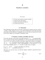
Fig. 24.1. An example of a finite difference grid {jh, ik}
N
x
, N
t
j=0,i=0
. Crosses mark
points used by the binomial method (24.13) to obtain a single time-zero option
value.
finite difference schemes for such problems; see (Wilmott et al., 1995), for exam-
ple. A promising, but often overlooked, alternative is to use a penalty method. In-
deed, the basic binomial method of Chapter 18 is an example of a simple, explicit
penalty method. More accurate versions are developed and analysed in (Forsyth
and Vetzal, 2002). Our illustration in Section 24.4 of the connection between bi-
nomial and finite difference methods was based on Appendix C of (Forsyth and
Vetzal, 2002). A fuller treatment of this topic can be found in (Kwok, 1998).
It is worth making the point that the development and implementation of nu-
merical methods for PDEs is an area where a beginner is generally best advised to
make use of existing technology: ‘off the shelf’ is preferable to ‘roll your own’.
However, a basic understanding of the nature of simple numerical methods, at the
level of these last two chapters, gives a good feel for what to expect from PDE
solvers.
MATLAB comes with a fairly simple built-in PDE solver,
pdepe, and may
be augmented with a PDE toolbox. Generally, there is an abundance of nu-

merical PDE software available, both commercially and in the public domain.
Good places to start are the Netlib Repository www.netlib.org/liblist.html and
the Differential Equations and Related Topics page dee.
ac.uk/software/index.html#DEs maintained by David Griffiths at the University
of Dundee.
264 Finite difference methods for the Black–Scholes PDE
%CH24 Program for Chapter 24
%
% Crank-Nicolson for a European put
clf
%%%%%%% Problem and method parameters %%%%%%%
E=4;sigma = 0.3;r=0.03;T=1;
L=10; Nx = 50; Nt = 50; k = T/Nt;h=L/Nx;
%%%%%%%%%%%%%%%%%%%%%%%%%%%%%%%%
T1 = diag(ones(Nx-2,1),1) - diag(ones(Nx-2,1),-1);
T2 = -2*eye(Nx-1,Nx-1) + diag(ones(Nx-2,1),1) + diag(ones(Nx-2,1),-1);
mvec = [1:Nx-1];
D1 = diag(mvec);
D2 = diag(mvec.ˆ2);
F=(1-r*k)*eye(Nx-1,Nx-1) + 0.5*k*sigmaˆ2*D2*T2 + 0.5*k*r*D1*T1;
B=(1+r*k)*eye(Nx-1,Nx-1) - 0.5*k*sigmaˆ2*D2*T2 - 0.5*k*r*D1*T1;
A1 = 0.5*(eye(Nx-1,Nx-1) + F);
A2 = 0.5*(eye(Nx-1,Nx-1) + B);
U=zeros(Nx-1,Nt+1);
U(:,1) = max(E-[h:h:L-h]’,0);
for i = 1:Nt
tau = (i-1)*k;
p1 = k*(0.5*sigmaˆ2 - 0.5*r)*E*exp(-r*(tau));
q1 = k*(0.5*sigmaˆ2 - 0.5*r)*E*exp(-r*(tau+k));
rhs = A1*U(:,i) + [0.5*(p1+q1); zeros(Nx-2,1)];

X=A2\rhs;
U(:,i+1) = X;
end
bca = E*exp(-r*[0:k:T]);
bcb = zeros(1,Nt+1);
U=[bca;U;bcb];
mesh([0:k:T],[0:h:L],U)
xlabel(’T-t’), ylabel(’S’), zlabel(’Put Value’)
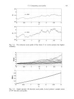
Fig. 24.2. Program of Chapter 24: ch24.m.
24.6 Program of Chapter 24 and walkthrough 265
EXERCISES
24.1.  Confirm that FTCS in (24.6) and BTCS in (24.7) have matrix–vector
forms (23.9) and (23.11), respectively, as indicated in Section 24.2.
24.2.  In the case of a European call option, point out a contradiction in the
initial and boundary conditions (24.2) and (24.4). How could this be over-
come?
24.3.  Write the FTCS, BTCS and Crank–Nicolson methods for a down-and-
out call option in matrix–vector form.
24.4. Confirm that the transformations given in Section 24.4 convert (8.15)
to (24.10).
24.5.  Suppose that a constant diffusion coefficient,
1
2
σ
2
,isintroduced into the
heat equation (23.2) to give
∂u
∂t
=

1
2
σ
2
∂
2
u
∂x
2
.
The FTCS method would then use
k
−1

t
U
i
j
−
1
2
h
−2
δ
2
x
U
i
j
= 0.

Show that the von Neumann stability condition takes the form σ
2
k ≤ h
2
.
24.6 Program of Chapter 24 and walkthrough
Our program ch24 implements Crank–Nicolson, (24.8), for a European put, producing a picture like
that in Figure 11.4. It is listed in Figure 24.2. The structure of the code is similar to ch23, and the
commands used have been explained in previous chapters.
PROGRAMMING EXERCISES
P24.1. Alter ch24 so that it values a down-and-out call option.
P24.2. Investigate the use of MATLAB’s built-in PDE solver
pdepe for option
valuation. Type
help pdepe or consult (Higham and Higham, 2000, Section 12.4)
for details of how to use
pdepe.
Quote
one reason I’ve found financial engineering so exciting
is that banks pay attention to a lot of academic work.
In that sense, it’s a very aggressive area,
because if you have a new method for solving a problem of interest,
there will be listeners.
And they’ll come back, ask questions, be on the phone,
and fill the seminar room.
TOM COLEMAN, Financial Engineering News, September/October 2002

References
Almgren, Robert F. (2002) Financial derivatives and partial differential equations.
American Mathematical Monthly, 109:1–12.

Andersen, L. and M. Broadie (2001) A primal–dual simulation algorithm for pricing
multi-dimensional American options. Working paper, University of Columbia, New
York.
Bass, Thomas A. (1999) The Predictors. London: Penguin.
Baxter, Martin and Andrew Rennie (1996) Financial Calculus: An Introduction to
Derivative Pricing. Cambridge: Cambridge University Press.
Bj
¨
ork, Thomas (1998) Arbitrage Theory in Continuous Time. Oxford: Oxford University
Press.
Black, Fischer (1989) How to use the holes in Black and Scholes. Journal of Applied
Corporate Finance, 1:4, Winter:67–73.
Black, F. and M. Scholes (1973) The pricing of options and corporate liabilities. Journal
of Political Economy, 81:637–659.
Boyle, P. P. (1977) Options: A Monte Carlo approach. Journal of Financial Economics,
4:323–338.
Boyle, Phelim, Mark Broadie and Paul Glasserman (1997) Monte Carlo methods for
security pricing. Journal of Economic Dynamics and Control, 21:1267–1321.
Broadie, Mark and Paul Glasserman (1998) Introduction to Chapter III: Volatility and
correlation. In Mark Broadie and Paul Glasserman, eds, Hedging with Trees.
London: Risk Books.
Brze
´
zniak, Zdislaw and Tomasz Zastawniak (1999) Basic Stochastic Processes. Berlin:
Springer.
Capi
´
nski, Marek and Ekkehard Kopp (1999) Measure, Integral and Probability. Berlin:
Springer.
Clewlow, Les and Chris Strickland (1998) Implementing Derivative Models. Chichester:

Wiley.
Cochrane, John H. (2001) Asset Pricing. Princeton, NJ: Princeton University Press.
Corless, Robert M. (2002) Essential Maple 7. Berlin: Springer.
Cox, John C., Stephen A. Ross, and Mark Rubinstein (1979) Option pricing: a simplified
approach. Journal of Financial Economics, 7:229–263.
Cyganowski, Sasha, Lars Gr
¨
une and Peter E. Kloeden (2002) MAPLE for jump–diffusion
stochastic differential equations in finance. In S. S. Nielsen, ed., Programming
Languages and Systems in Computational Economics and Finance, Boston, MA:
Kluwer, pp. 441–460.
267
268 References
Dalton, John (ed.) (2001) How the Stock Market Works, 3rd edn. Englewood Cliffs, NJ:
Prentice Hall Press.
Denney, Mark and Steven Gaines (2000) Chance in Biology,Princeton, NJ: Princeton
University Press.
Duffie, Darrell (2001) Dynamic Asset Pricing Theory, 3rd edn. Princeton, NJ: Princeton
University Press.
Elder, Alexander (2002) Come into My Trading Room: a Complete Guide to Trading.
Chichester: Wiley.
Estep, Donald (2002) Practical Analysis in One Variable. Berlin: Springer.
Farmer, J. Doyne (1999) Physicists attempt to scale the ivory towers of finance.
Computing in Science and Engineering,November:26–39.
Forsyth, P. A. and K. R. Vetzal (2002) Quadratic convergence for valuing American
options using a penalty method. SIAM Journal on Scientific Computing,
23:2095–2122.
Fr
¨
oberg, Carl-Erik (1985) Numerical Mathematics. Menlo Park, CA:

Benjamin/Cummings.
Fu, M., S. Laprise, D. Madan, Y. Su. and R. Wu (2001) Pricing American options: a
comparison of Monte Carlo simulation approaches. Journal of Computational
Finance, 4:39–88.
Gard, Thomas C. (1988) Introduction to Stochastic Differential Equations.New York:
Marcel Dekker.
Goodman, Jonathan and Daniel N. Ostrov (2002) On the early exercise boundary of the
American put option. SIAM Journal on Applied Mathematics, 62:1823–1835.
Green, T. Clifton and Stephen Figlewski (1999) Market risk and model risk for a financial
institution writing options. Journal of Finance, 53:1465–1499.
Grimmett, Geoffrey and David Stirzaker (2001) Probability and Random Processes,
Oxford: Oxford University Press.
Grimmett, Geoffrey and Dominic Welsh (1986) Probability. An Introduction. Oxford:
Oxford University Press.
Grinstead, Charles M. and J. Laurie Snell (1997) Introduction to Probability. Providence,
RI: American Mathematical Society.
Hammersley, J. M. and D. C. Handscombe (1964) Monte Carlo Methods. London:
Methuen.
Heath, Michael T. (2002) Scientific Computing: An Introductory Survey, 3rd edn. New
York: McGraw-Hill.
Higham, Desmond J. (2001) An algorithmic introduction to numerical simulation of
stochastic differential equations. SIAM Review, 43:525–546.
Higham, Desmond J. (2002) Nine ways to implement the binomial method for option
valuation in MATLAB. SIAM Review, 44:661–677.
Higham, Desmond J. and Nicholas J. Higham (2000) MATLAB Guide. Philadelphia, PA:
SIAM.
Higham, Desmond J. and Peter E. Kloeden (2002) MAPLE and MATLAB for stochastic
differential equations in finance. In S. S. Nielsen, ed., Programming Languages and
Systems in Computational Economics and Finance, pp. 233–269. Boston, MA:
Kluwer.

Hull, John C. (2000) Options, Futures, and Other Derivatives,4th edn. Englewood Cliffs,
NJ: Prentice-Hall.
Hull, J. C. and A. White (1987) The pricing of options on assets with stochastic
volatilities. Journal of Finance, 42:281–300.
Isaac, Richard (1995) The Pleasures of Probability. Berlin: Springer.
References 269
Iserles, Arieh (1996) A First Course in the Numerical Analysis of Differential Equations.
Cambridge: Cambridge University Press.
J
¨
ackel, Peter (2002) Monte Carlo Methods in Finance. Chichester: Wiley.
Johnson, Philip McBride (1999) Derivatives, a Manager’s Guide to the World’s Most
Powerful Financial Instruments. Columbus, OH: McGraw-Hill.
Karatzas, I. and S. Shreve (1998) Methods of Mathematical Finance.New York: Springer.
Kelley, C. T. (1995) Iterative Methods for Linear and Nonlinear Equations. Philadelphia,
PA: SIAM.
Kloeden, Peter E. and Eckhard Platen (1992) Numerical Solution of Stochastic
Differential Equations. Berlin: Springer (corrected 1999).
Kritzman, Mark. P. (2000) Puzzles of Finance: Six Practical Problems and Their
Remarkable Solutions. Chichester: Wiley.
Kuske, R. and J. B. Keller (1998) Optimal exercise boundary for an American put option.
Applied Mathematical Finance, 5:107–116.
Kwok, Y. K. (1998) Mathematical Models of Financial Derivatives. Berlin: Springer.
Leisen, Dietmar P. J. (1998) Pricing the American put: a detailed convergence analysis for
binomial methods. Journal of Economic Dynamics and Control, 22:1419–1444.
Leisen, Dietmar and Matthias Reimer (1996) Binomial models for option valuation –
examining and improving convergence. Applied Mathematical Finance, 3:319–346.
Lewis, Michael (1989) Liar’s Poker. London: Hodder & Stoughton.
Lo, Andrew W. and Craig MacKinlay (1999) A Non-Random Walk Down Wall Street.
Princeton, NJ: Princeton University Press.

Longstaff, F. A. and E. S. Schwartz (2001) Valuing American options by simulation: a
simple least-squares approach. Review of Financial Studies, 14:113–147.
Lowenstein, Roger (2001) When Genius Failed. London: Fourth Estate.
Madan, Dilip B. (2001) On the modelling of option prices. Quantitative Finance,1.
Madras, Neal (2002) Lectures on Monte Carlo Methods. Providence, RI: American
Mathematical Society.
Malkiel, Burton G. (1990) A Random Walk down Wall Street.New York: Norton.
Manaster, S. and G. Koehler (1982) The calculation of implied variances from the
Black–Scholes model: a note. Journal of Finance, 38:227–230.
Mantegna, Rosario N. and H. Eugene Stanley (2000) An Introduction to Econophysics:
Correlations and Complexity in Finance. Cambridge: Cambridge University Press.
Mao, Xuerong (1997) Stochastic Differential Equations and Applications. Chichester:
Horwood.
Merton, R. C. (1973) Theory of rational option pricing. Bell Journal of Economics and
Management Science, 4:141–183.
Mitchell, A. R. and D. F. Griffiths (1980) The Finite Difference Method in Partial
Differential Equations. Chichester: Wiley.
Morgan, Byron J. T. (2000) Applied Stochastic Modelling. London: Arnold.
Morton, K. W. and D. F. Mayers (1994) Numerical Solution of Partial Differential
Equations. Cambridge: Cambridge University Press.
Nahin, Paul J. (2000) Duelling Idiots and Other Probability Puzzlers. Princeton, NJ:
Princeton University Press.
Nielsen, Lars Tyge (1999) Pricing and Hedging of Derivative Securities. Oxford: Oxford
University Press.
Øksendal, Bernt (1998) Stochastic Differential Equations, 5th edn. Berlin: Springer.
Ortega, J. M. and W. C. Rheinboldt (1970) Iterative Solution of Nonlinear Equations in
Several Variables.PA: re-published by Society for Industrial and Applied
Mathematics, Philadelphia, in 2000.
270 References
Poon, S H. and C. Granger (2003) Forecasting volatility in financial markets. Journal of

Economic Literature,toappear.
Rebonato, Riccardo (1999) Volatility and Correlation: In the Pricing of Equity, FX and
Interest-Rate Options. Chichester: Wiley.
Ripley, B. D. (1997) Stochastic Simulation. Chichester: Wiley.
Rogers, L. C. G. (2002) Monte Carlo valuation of American options. Mathematical
Finance, 12:271–286.
Rogers, L. C. G. and E. J. Stapleton (1998) Fast accurate binomial pricing of options.
Finance and Stochastics, 2:3–17.
Rogers, L. C. G. and O. Zane (1999) Saddle-point approximations to option prices.
Annals of Applied Probability, 9:493–503.
Rosenthal, Jeffrey S. (2000) A First Look at Rigorous Probability Theory. Singapore:
World Scientific.
Seydel, Rudiger (2002) Tools for Computational Finance. Berlin: Springer.
Smith, A. L. H. (1986) Trading Financial Options. London: Butterworths.
Strikwerda, J. C. (1989) Finite Difference Schemes and Partial Differential Equations.
Belnout, CA: Wadsworth and Brooks/Cole.
Taleb, Nassim (1997) Dynamic Hedging: Managing Vanilla and Exotic Options.
Chichester: Wiley.
Walker, Joseph A. (1991) How the Options Markets Work. Englewood Cliffs, NJ:
Prentice-Hall Press.
Walsh, John B. (2003) The rate of convergence of the binomial tree scheme. Finance and
Stochastics,toappear.
Wilmott, Paul (1998) Derivatives. Chichester: Wiley.
Wilmott, Paul, Sam Howison and Jeff Dewynne (1995) The Mathematics of Financial
Derivatives. Cambridge: Cambridge University Press.
Index
American option, 6, 7, 151, 173–182, 196
optimal exercise boundary, 177–179
American Stock Exchange, 50
antithetic variates, see variance reduction

arbitrage, 13, 17–19, 106, 116, 120, 132, 174, 175
ARCH, see autoregressive conditional
heteroscedasticity
Asian option, 192–194, 196
ask price, 4
asset model
continuous, 56, 59, 60
discrete, 54, 55, 60, 151
incremental, 56
mean, 56, 60, 64
second moment, 56, 60
timescale invariance, 66–69
variance, 56, 60
asset-or-nothing option, 169
at-the-money, 88, 89, 108, 110, 164, 166, 167
autoregressive conditional heteroscedasticity, 209
average price Asian call, 192, 231–232
average price Asian put, 192, 194
average strike Asian call, 192
average strike Asian put, 193
backward difference, 243, 262
barrier option, 187–191, 196, 197
Bermudan option, 193–194, 196
Bernoulli random variable, 22, 24, 153
bid price, 4
bid–ask spread, 5, 6, 10, 49, 205
binary option, see also cash-or-nothing option 164
binomial method, 118, 151–156
as a finite difference method, 157, 261–263
convergence, 156

for American put, 176–177
for exotics, 194–196
for Greeks, 157, 159
oscillation, 156, 157, 262
bisection method, 123–125, 127, 131, 132
for implied volatility, 133
Black–Scholes formula, 80–82, 105,
131
cash-or-nothing, 164–166
down-and-out call, 189
European call, 81, 83, 89
European put, 81, 83, 92
geometric average price Asian call, 198
up-and-out call, 190
Black–Scholes formulas, 82, 83
Black–Scholes PDE, 73, 78, 80, 81, 83, 99, 101–103,
165, 166, 239, 251, 257–262
American put, 174–176
barrier option, 190
down-and-out call, 188, 189
exotic option, 196
bottom straddle, 4, 8
Brownian motion, 61, 70
geometric, 57, 61
bull spread, 4, 8
butterfly spread, 8, 17, 83
cash-or-nothing call option, 163–168
CBOE, see Chicago Board Options Exchange
central difference, 262
Central Limit Theorem, 27–28, 38, 54, 55, 68, 74, 75,

142, 144, 154
Chicago Board Options Exchange, 4, 50
confidence interval, 57, 58, 60
historical volatility, 204, 205, 210
Monte Carlo method, 142–143, 145, 146, 181, 194,
195, 215, 218, 219, 221, 224, 225, 230, 231, 233
continuous random variable, 22
continuous time asset model, 56, 59, 60, 154
continuously compounded rate of return, 70
control variates, 229 see also variance reduction
convergence in distribution, 27
correlated random variables, 146
covariance, 217, 225, 230
daily returns, 46
delta, 99–102, 108
of a European call, 87
of a European put, 87
delta hedging, 87, 99, 106, 167
derivatives, financial, 7
digital option, 164 see also cash-or-nothing option
discounting for interest, 12, 153
discrete asset path, 63, 64
discrete hedging, 88
discrete random variable, 21
discrete time asset model, 54, 55, 60, 158
discrete time asset path, 63–66
distribution function, 26
271
272 Index
dividends, 49, 182

double barrier option, 191
down-and-in call, 188, 189
down-and-in put, 190
down-and-out call, 187–189, 260–261, 265
down-and-out put, 190
drift, 54, 105, 198
efficient market hypothesis, 45–46, 49, 51, 52, 54, 61,
70, 72
error bar, 143
error function, 41
inverse, 41
European call option, 163
definition, 1
delta, 87
European put option
definition, 2
delta, 87
European-style option, 115, 144, 146, 152
EWMA, see exponentially weighted moving
average
exercise price, 1
exercise strategy, 180, 181, 183
exotic option, 7, 187–196, 222
expected payoff, 115–116, 118–120
expected value, 21, 22
expiry date, 1
exponential distribution, 29, 41
exponentially weighted moving average, 208
fat tails, 70
financial derivatives, 7

Financial Times, 5, 135
finite difference approximation, 146
finite difference method, 237–251
available software, 263
BTCS, 240–247, 249, 252, 257–261, 265
convergence, 247–249, 260
Crank–Nicolson, 249–252, 257–261, 265
for American option, 263
for Black–Scholes PDE, 257–260
FTCS, 240–249, 252, 257–260, 265
instability, 243
local accuracy, 246–247, 249, 251, 252
penalty method, 263
stencil, 242, 244, 249
upwind, 262
von Neumann stability, 247–249, 251, 252, 260,
265
finite difference operator, 237–238, 240, 251
finite element method, 251
fixed strike lookback call, 192
fixed strike lookback put, 192
floating strike lookback call, 192
floating strike lookback put, 192, 199
forward contract, 17, 83
forward difference, 238, 241, 243
free boundary problem, 182
FTSE 100 index, 135
futures contract, 17
gamma, 99, 100
GARCH, generalized autoregressive conditional

heteroscedasticity, 209
geometric average price Asian call, 197, 198
geometric Brownian motion, 57, 61
geometrically declining weights, 208, 210
Greeks, 99–102
grid, 239
heat equation, 238–239, 262, 265
hedging, 74, 76–78, 82, 87–93, 106, 116, 145, 164,
188
historical volatility, 203–209
IBM daily data, 208
IBM weekly data, 208
maximum likelihood, 206–207, 210
Monte Carlo, 203–206
hockey stick, 3, 106, 111, 177, 179
i.i.d., 23, 28, 48, 54, 58, 59, 215, 220
illiquidity, 94
implied volatility, 99, 123, 131–137, 203
in-the-money, 88–91, 108, 110, 163, 164, 167,
174
independence, 23–24, 216
independent and identically distributed, see i.i.d.
interest rate, 11–12, 16, 53
kernel density estimation, 36, 38, 40, 48, 66
Law of the Iterated Logarithm, 59
Lax Equivalence Theorem, 248, 251
LIFFE, see London International Financial Futures &
Options Exchange
linear complementarity problem, 175, 182
liquidity, 94

log ratio, 48, 203, 210
lognormal distribution, 56, 57, 59, 60, 66, 70, 118
London International Financial Futures and Options
Exchange, 5, 135
London Stock Exchange, 50
Long-Term Capital Management, 93–94
lookback option, 191–192, 196
low discrepancy sequences, 233
market makers, 4
martingale, 118
MATLAB toolboxes, xiv
maximum likelihood principle, 206–207
mean, 21, 22
mesh, 239
mesh ratio, 241, 249
missing data, 49
moneyness ratio, 110
monotonic decreasing function, 220
monotonic increasing function, 220, 225
Monte Carlo method, 141–148, 215–224,
229–232
for American put, 180–182
for exotics, 194–196
for Greeks, 145–148
Index 273
New York Stock Exchange, 6, 50
Newton’s method, 124–128, 131–133
normal distribution, normal random variable, 25–27,
29, 142, 203, 221
optimal exercise boundary, 182, 183

OTC, see over-the-counter
out-of-the-money, 88–91, 108, 110, 167, 173
over-the-counter,
Parisian option, 191
partial barrier option, 191
partial differential equation, 73, see also PDE
path-dependency, 187
payoff diagram, 3
bottom straddle, 4
bull spread, 4
cash-or-nothing call, 164
cash-or-nothing put, 164
European call, 3
European put, 3
PDE see Black–Scholes PDE
Prediction Company, The, 70
pseudo-random numbers, 33–34, 40, 43, 48, 63, 64,
88, 141, 145, 148, 205, 218, 219, 225, 230, 231
put–call parity, 13–14, 17, 83, 102, 131
cash-or-nothing, 165, 169
put–call supersymmetry, 111
quadratic convergence, 125
quadrature method, 232
quantile, 36
quantile–quantile plot, 37, 38, 48
quasi Monte Carlo, 233
random number generators, 33 see also
pseudo-random numbers
replicating portfolio, 76–78, 167, 174
return, 46, 48, 68

rho, 99, 101
risk-neutral investor, 118
risk-neutral world, 118, 119
risk neutrality, 115, 118–120, 144, 146, 151, 154, 163,
167, 180, 181, 194, 232
cash-or-nothing, 167–168
sample mean, 34, 48, 64, 141, 146,
204, 215
sample variance, 34, 48
SDE, see stochastic differential equation
second order central difference, 241
second order convergence, 125
self-financing portfolio, 78
short selling, 12, 19, 77, 174, 175
shout option, 193–194, 196
spread
bull, 4, 8
butterfly, 8, 10, 17, 83
pterodactyl, 10
standard deviation, 24
stochastic differential equation, 57, 59
stopping time, 180
straddle
bottom, 4, 8
O’Hare, 19
strike price, 1
Strong Law of Large Numbers, 59
sum-of-square returns, 68–69
theta, 99, 101, 102
traders’ rule-of-thumb, 58, 60

true random numbers, 40
unbiased, 142, 148
uniform distribution, 22, 24, 28
up-and-in call, 190, 223
up-and-in put, 190
up-and-out call, 190, 194, 195, 197
up-and-out put, 190
variance, 24, 142
variance reduction, 143, 232
and hedging, 233
antithetic variates, 215–224
control variates, 229–232
vega, 99, 101, 102, 132
volatility, 54, 59, 64, 70, 105, 110, 111, 131, 198,
262
implied, see implied volatility
scaled, 110
volatility frown, 137
volatility smile, 137
Wall Street Journal,6,31, 62
website for this book, xiii
weekly returns, 48