An Introduction to Financial Option Valuation: Mathematics, Stochastics and Computation_1 pot

This page intentionally left blank
AN INTRODUCTION TO FINANCIAL
OPTION VALUATION
Mathematics, Stochastics and Computation
This is a lively textbook providing a solid introduction to financial option valuation
for undergraduate students armed with only a working knowledge of first year
calculus. Written as a series of short chapters, this self-contained treatment gives
equal weight to applied mathematics, stochastics and computational algorithms,
with no prior background in probability, statistics or numerical analysis required.
Detailed derivations of both the basic asset price model and the Black–Scholes
equation are provided along with a presentation of appropriate computational tech-
niques including binomial, finite differences and, in particular, variance reduction
techniques for the Monte Carlo method.
Each chapter comes complete with accompanying stand-alone MATLAB code
listing to illustrate a key idea. The author has made heavy use of figures and ex-
amples, and has included computations based on real stock market data. Solutions
to exercises are made available at www.cambridge.org.
D
ES HIGHAM is a professor of mathematics at the University of Strathclyde. He
has co-written two previous books, MATLAB Guide and Learning LaTeX.In2005
he was awarded the Germund Dahlquist Prize by the Society for Industrial and
Applied Mathematics for his research contributions to a broad range of problems
in numerical analysis.

AN INTRODUCTION TO FINANCIAL
OPTION VALUATION
Mathematics, Stochastics and Computation
DESMOND J. HIGHAM
Department of Mathematics
University of Strathclyde

CAMBRIDGE UNIVERSITY PRESS
Cambridge, New York, Melbourne, Madrid, Cape Town, Singapore, São Paulo
Cambridge University Press
The Edinburgh Building, Cambridge CB2 8RU, UK
First published in print format
ISBN-13 978-0-521-83884-9
ISBN-13 978-0-521-54757-4
ISBN-13 978-0-511-33704-8
© Cambridge University Press 2004
2004
Information on this title: www.cambridge.org/9780521838849
This publication is in copyright. Subject to statutory exception and to the provision of
relevant collective licensing agreements, no reproduction of any part may take place
without the written
p
ermission of Cambrid
g
e University Press.
ISBN-10 0-511-33704-3
ISBN-10 0-521-83884-3
ISBN-10 0-521-54757-1
Cambridge University Press has no responsibility for the persistence or accuracy of urls
for external or third-party internet websites referred to in this publication, and does not
g
uarantee that any content on such websites is, or will remain, accurate or a
pp
ro
p
riate.
Published in the United States of America by Cambridge University Press, New York

www.cambridge.org
hardback
paperback
paperback
eBook (EBL)
eBook (EBL)
hardback
To my family,
Catherine, Theo, Sophie and Lucas

Contents
List of illustrations page xiii
Preface xvii
1 Options 1
1.1 What are options? 1
1.2 Why do we study options? 2
1.3 How are options traded? 4
1.4 Typical option prices 6
1.5 Other financial derivatives 7
1.6 Notes and references 7
1.7 Program of Chapter 1 and walkthrough 8
2 Option valuation preliminaries 11
2.1 Motivation 11
2.2 Interest rates 11
2.3 Short selling 12
2.4 Arbitrage 13
2.5 Put–call parity 13
2.6 Upper and lower bounds on option values 14
2.7 Notes and references 16
2.8 Program of Chapter 2 and walkthrough 17

3 Random variables 21
3.1 Motivation 21
3.2 Random variables, probability and mean 21
3.3 Independence 23
3.4 Variance 24
3.5 Normal distribution 25
3.6 Central Limit Theorem 27
3.7 Notes and references 28
3.8 Program of Chapter 3 and walkthrough 29
vii
viii Contents
4 Computer simulation 33
4.1 Motivation 33
4.2 Pseudo-random numbers 33
4.3 Statistical tests 34
4.4 Notes and references 40
4.5 Program of Chapter 4 and walkthrough 41
5 Asset price movement 45
5.1 Motivation 45
5.2 Efficient market hypothesis 45
5.3 Asset price data 46
5.4 Assumptions 48
5.5 Notes and references 49
5.6 Program of Chapter 5 and walkthrough 50
6 Asset price model: Part I 53
6.1 Motivation 53
6.2 Discrete
asset model 53
6.3 Continuous asset model 55
6.4 Lognormal distribution 56

6.5 Features of the asset model 57
6.6 Notes and references 59
6.7 Program of Chapter 6 and walkthrough 60
7 Asset price model: Part II 63
7.1 Computing asset paths 63
7.2 Timescale invariance 66
7.3 Sum-of-square returns 68
7.4 Notes and references 69
7.5 Program of Chapter 7 and walkthrough 71
8 Black–Scholes PDE and formulas 73
8.1 Motivation 73
8.2 Sum-of-square increments for asset price 74
8.3 Hedging 76
8.4 Black–Scholes PDE 78
8.5 Black–Scholes formulas 80
8.6 Notes and references 82
8.7 Program of Chapter 8 and walkthrough 83
Contents ix
9 More on hedging 87
9.1 Motivation 87
9.2 Discrete hedging 87
9.3 Delta at expiry 89
9.4 Large-scale test 92
9.5 Long-Term Capital Management 93
9.6 Notes 94
9.7 Program of Chapter 9 and walkthrough 96
10 The Greeks 99
10.1 Motivation 99
10.2 The Greeks 99
10.3 Interpreting the Greeks 101

10.4 Black–Scholes PDE solution 101
10.5 Notes and references 102
10.6 Program of Chapter 10 and walkthrough 104
11 Mor
e on the Black–Scholes formulas
105
11.1 Motivation 105
11.2 Where is µ? 105
11.3 Time dependency 106
11.4 The big picture 106
11.5 Change of variables 108
11.6 Notes and references 111
11.7 Program of Chapter 11 and walkthrough 111
12 Risk neutrality 115
12.1 Motivation 115
12.2 Expected payoff 115
12.3 Risk neutrality 116
12.4 Notes and references 118
12.5 Program of Chapter 12 and walkthrough 120
13 Solving a nonlinear equation 123
13.1 Motivation 123
13.2 General problem 123
13.3 Bisection 123
13.4 Newton 124
13.5 Further practical issues 127
x Contents
13.6 Notes and references 127
13.7 Program of Chapter 13 and walkthrough 128
14 Implied volatility 131
14.1 Motivation 131

14.2 Implied volatility 131
14.3 Option value as a function of volatility 131
14.4 Bisection and Newton 133
14.5 Implied volatility with real data 135
14.6 Notes and references 137
14.7 Program of Chapter 14 and walkthrough 137
15 Monte Carlo method 141
15.1 Motivation 141
15.2 Monte Carlo 141
15.3 Monte Carlo
for option valuation 144
15.4 Monte Carlo for Greeks 145
15.5 Notes and references 148
15.6 Program of Chapter 15 and walkthrough 149
16 Binomial method 151
16.1 Motivation 151
16.2 Method 151
16.3 Deriving the parameters 153
16.4 Binomial method in practice 154
16.5 Notes and references 156
16.6 Program of Chapter 16 and walkthrough 159
17 Cash-or-nothing options 163
17.1 Motivation 163
17.2 Cash-or-nothing options 163
17.3 Black–Scholes for cash-or-nothing options 164
17.4 Delta behaviour 166
17.5 Risk neutrality for cash-or-nothing options 167
17.6 Notes and references 168
17.7 Program of Chapter 17 and walkthrough 170
18 American options 173

18.1 Motivation 173
18.2 American call and put 173
Contents xi
18.3 Black–Scholes for American options 174
18.4 Binomial method for an American put 176
18.5 Optimal exercise boundary 177
18.6 Monte Carlo for an American put 180
18.7 Notes and references 182
18.8 Program of Chapter 18 and walkthrough 183
19 Exotic options 187
19.1 Motivation 187
19.2 Barrier options 187
19.3 Lookback options 191
19.4 Asian options 192
19.5 Bermudan and shout options 193
19.6 Monte Carlo and binomial for exotics 194
19.7 Notes and references 196
19.8 Program of Chapter 19 and walkthrough 199
20 Historical volatility 203
20.1 Motivation 203
20.2 Monte Carlo-type estimates 203
20.3 Accuracy of the sample variance estimate 204
20.4 Maximum likelihood estimate 206
20.5 Other volatility estimates 207
20.6 Example with real data 208
20.7 Notes and references 209
20.8 Program of Chapter 20 and walkthrough 210
21 Monte Carlo Part II: variance reduction by
antithetic variates 215
21.1 Motivation 215

21.2 The big picture 215
21.3 Dependence 216
21.4 Antithetic variates: uniform example 217
21.5 Analysis of the uniform case 219
21.6 Normal case 221
21.7 Multivariate case 222
21.8 Antithetic variates in option valuation 222
21.9 Notes and references 225
21.10 Program of Chapter 21 and walkthrough 225
xii Contents
22 Monte Carlo Part III: variance reduction by control variates 229
22.1 Motivation 229
22.2 Control variates 229
22.3 Control variates in option valuation 231
22.4 Notes and references 232
22.5 Program of Chapter 22 and walkthrough 234
23 Finite difference methods 237
23.1 Motivation 237
23.2 Finite difference operators 237
23.3 Heat equation 238
23.4 Discretization 239
23.5 FTCS and BTCS 240
23.6 Local accuracy 246
23.7 Von Neumann stability and convergence 247
23.8 Crank–Nicolson 249
23.9 Notes and references 251
23.10 Program of Chapter 23 and walkthrough 252
24 Finite difference methods for the Black–Scholes PDE 257
24.1 Motivation 257
24.2 FTCS, BTCS and Crank–Nicolson for Black–Scholes 257

24.3 Down-and-out call example 260
24.4 Binomial method as finite differences 261
24.5 Notes and references 262
24.6 Program of Chapter 24 and walkthrough 265
References 267
Index 271
Illustrations
1.1 Payoff diagram for a European call. page 3
1.2 Payoff diagram for a European put. 4
1.3 Payoff diagram for a bull spread. 5
1.4 Market values for IBM call and put options. 6
1.5 Another view of market values for IBM call and put options. 7
1.6 Program of Chapter 1:
ch01.m.9
2.1 Upper and lower bounds for European call option. 15
2.2 Program of Chapter 2:
ch02.m.18
2.3 Figure produced by
ch02.m.19
3.1 Density function for an N(0, 1) random variable. 25
3.2 Density functions for various N(µ, σ
2
) random variables. 26
3.3 N(0, 1) density and distribution function N (x).27
3.4 Program of Chapter 3:
ch03.m.30
3.5 Graphics produced by
ch03.31
4.1 Kernel density estimate. 36
4.2 Kernel density estimate with increasing number of samples. 37

4.3 Quantiles for a normal distribution. 38
4.4 Quantile–quantile plots. 39
4.5 Kernel density estimate illustrating Central Limit Theorem. 39
4.6 Quantile–quantile plot illustrating Central Limit Theorem. 40
4.7 Program of Chapter 4:
ch04.m.42
5.1 Daily IBM share price. 46
5.2 Weekly IBM share price. 47
5.3 Statistical tests of IBM share price data. 47
5.4 Program of Chapter 5:
ch05.m.51
6.1 Two lognormal density plots. 57
6.2 Program of Chapter 6:
ch06.m.61
7.1 Discrete asset path. 64
7.2 Two discrete asset paths with different volatility. 65
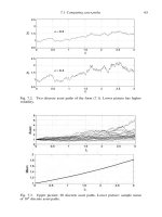
7.3 Twenty discrete asset paths and sample mean. 65
7.4 Fifty discrete asset paths and final time histogram. 66
xiii
xiv List of illustrations
7.5 The same asset path sampled at different scales. 67
7.6 Asset paths and running sum-of-square returns. 69
7.7 Program of Chapter 7:
ch07.m.71
8.1 Asset paths and running sum-of-square increments. 76
8.2 Program of Chapter 8:
ch08.m.84
9.1 Discrete hedging simulation: expires in-the-money. 90
9.2 Discrete hedging simulation: expires out-of-the-money. 91
9.3 Discrete hedging simulation: expires almost at-the-money. 92

9.4 Large-scale discrete hedging example. 93
9.5 Program of Chapter 9:
ch09.m.95
10.1 Program of Chapter 10:
ch10.m. 103
11.1 Option value in terms of asset price at five different times. 107
11.2 Three-dimensional version of Figure 11.1. 107
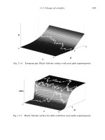
11.3 European call: Black–Scholes surface with asset path superimposed. 108
11.4 European put: Black–Scholes surface with asset path superimposed. 109
11.5 Black–Scholes surface for delta with asset paths superimposed. 109
11.6 Program of Chapter 11:
ch11.m. 112
12.1 Time-zero discounted expected call payoff and Black–Scholes value. 117
12.2 Program of Chapter 12:
ch12.m. 121
13.1 The function F(x) := N (x) −
2
3
. 126
13.2 Error in the bisection method and Newton’s method. 126
13.3 Program of Chapter 13:
ch13.m. 128
14.1 Newton’s method for the implied volatility. 135
14.2 Implied volatility against exercise price for some FTSE 100 index
data. 136
14.3 Program of Chapter 14:
ch14.m. 138
15.1 Monte Carlo approximations to
E(e
Z

), where Z ∼ N(0, 1). 143
15.2 Monte Carlo approximations to a European call option value. 145
15.3 Monte Carlo approximations to time-zero delta of a European
call option. 147
15.4 Program of Chapter 15:
ch15.m. 149
16.1 Recombining binary tree of asset prices. 152
16.2 Convergence of the binomial method. 155
16.3 Error in the binomial method. 157
16.4 Program of Chapter 16:
ch16.m. 160
17.1 Payoff diagrams for cash-or-nothing call and put. 164
17.2 Black–Scholes surface for a cash-or-nothing call, with asset path
superimposed. 166
17.3 Black–Scholes delta surface for a cash-or-nothing call, with asset
path superimposed. 168
List o
f illustrations
xv
17.4 Program of Chapter 17: ch17.m.170
18.1 Convergence of the binomial method for an American put. 177
18.2 Error in binomial method for an American put. 178
18.3 Value P
Am
(S, T/4) for an American put, computed via the
binomial method. 178
18.4 Exercise boundary for an American put. 179
18.5 Monte Carlo approximations to the discounted expected American
put payoff with a simple exercise strategy. 181
18.6 Program of Chapter 18:

ch18.m.184
19.1 Two asset paths and a barrier. 188
19.2 Time-zero down-and-out call value. 189
19.3 Time-zero up-and-out call value. 191
19.4 Program of Chapter 19:
ch19.m.200
20.1 Historical volatility estimates for IBM data. 209
20.2 Program of Chapter 20:
ch20.m.211
20.3 Figure produced by
ch20.212
21.1 A pair of discrete asset paths computed using antithetic variates. 223
21.2 Program of Chapter 21:
ch21.m.226
22.1 Program of Chapter 22:
ch22.m.235
23.1 Heat equation solution. 240
23.2 Finite difference grid. 241
23.3 Stencil for FTCS. 242
23.4 FTCS solution on the heat equation: ν ≈ 0.3. 244
23.5 FTCS solution on the heat equation: ν ≈ 0.63. 245
23.6 Stencil for BTCS. 246
23.7 BTCS solution on the heat equation: ν ≈ 6.6. 247
23.8 Stencil for Crank–Nicolson. 250
23.9 Program of Chapter 23:
ch23.m.253
24.1 Finite difference grid relevant to binomial method. 263
24.2 Program of Chapter 24:
ch24.m.264

Preface
The aim of this book is to present a lively and palatable introduction to financial
option valuation for undergraduate students in mathematics, statistics and related
areas. Prerequisites have been kept to a minimum. The reader is assumed to have a
basic competence in calculus up to the level reached by a typical first year mathe-
matics programme. No background in probability, statistics or numerical analysis
is required, although some previous exposure to material in these areas would un-
doubtedly make the text easier to assimilate on first reading.
The contents are presented in the form of short chapters, each of which could
reasonably be covered in a one hour teaching session. The book grew out of a final
year undergraduate class called The Mathematics of Financial Derivatives that I
have taught, in collaboration with Professor Xuerong Mao, at the University of
Strathclyde. The class is aimed at students taking honours degrees in Mathematics
or Statistics, or joint honours degrees in various combinations of Mathematics,
Statistics, Economics, Business, Accounting, Computer Science and Physics. In
my view, such a class has two great selling points.
• From a student perspective, the topic is generally perceived as modern, sexy and likely
to impress potential employers.
• From the perspective of a university teacher, the topic provides a focus for ideas from
mathematical modelling, analysis, stochastics and numerical analysis.
There are many excellent books on option valuation. However, in preparing
notes for a lecture course, I formed the opinion that there is a niche for a single,
self-contained, introductory text that gives equal weight to
• applied mathematics,
• stochastics, and
• computational algorithms.
The classic applied mathematics view is provided by Wilmott, Howison and
Dewynne’s text (Wilmott et al., 1995). My aim has been to write a book at a sim-
ilar level with a less ambitious scope (only option valuation is considered), less
xvii

xviii Preface
emphasis on partial differential equations, and more attention paid to stochastic
modelling and simulation.
Key features of this book are as follows.
(i) Detailed derivation and discussion of the basic lognormal asset price model.
(ii) Roughly equal weight given to binomial, finite difference and Monte Carlo methods.
In particular, variance reduction techniques for Monte Carlo are treated in some detail.
(iii) Heavy use of computational examples and figures as a means of illustration.
(iv) Stand-alone MATLAB codes, with full listings and comprehensive descriptions, that
implement the main algorithms. The core text can be read independently of the codes.
Readers who are familiar with other programming languages or problem-solving en-
vironments should
have little difficulty in translating these examples.
In a nutshell, this is the book that I wish had been available when I started to
prepare lectures for the Strathclyde class.
When designing a text like this, an immediate issue is the level at which stochas-
tic calculus is to be treated. One of the tenets of this book is that
rigorous, measure-theoretic, stochastic analysis, although beautiful, is hard and it is
unrealistic to ask an undergraduate class to pick up such material on the fly. Monte
Carlo-style simulation, on the other hand, is a relatively simple concept, and well-
chosen computational experiments provide an excellent way to back up heuristic
arguments.
Hence, the approach here is to treat stochastic calculus on a nonrigorous level
and give plenty of supporting computational examples. I rely heavily on the Cen-
tral Limit Theorem as a basis for heuristic arguments. This involves a deliberate
compromise – convergence in distribution must be swapped for a stronger type of
convergence if these arguments are to be made rigorous – but I feel that erring on
the side of accessibility is reasonable, given the aims of this text.
In fact, in deriving the Black–Scholes partial differential equation, I do not make
explicit reference to It

ˆ
o’s Lemma. I decided that a heuristic derivation of It
ˆ
o’s
Lemma in a general setting followed by a single application of the lemma in one
simple case makes less pedagogical sense than a direct ‘in situ’ heuristic treatment,
a decision inspired by Almgren’s expository article (Almgren, 2002). I hope that
at least some undergraduate readers will be sufficiently motivated to follow up on
the references and become exposed to the real thing.
You can get a feeling for the contents of the book by skimming through the
outline bullet points that appear at the start of each chapter. Many of the later
chapters can be read independently of each other, or, of course, omitted.
Exercises are given at the end of each chapter. It is my experience that active
problem solving is the best learning tool, so I strongly encourage students to make
use of them. I have used a starring system: one star for questions whose solution
Preface xix
is relatively easy/short, rising to three stars for the hardest/longest questions. Brief
solutions to the odd-numbered exercises are available from the book website given
below. This leaves the even-numbered questions as a teaching resource. Certain
questions are central to the text. I have tried to ensure that these come up in the
odd-numbered list, in order to aid independent study.
A short, introductory treatment like this can only scratch the surface. Hence,
each chapter concludes with a Notes and references section, which gives my own,
necessarily biased, hints about important omissions. References can be followed
up via the References section at the end of the book.
Scattered at the end of each chapter are a few quotes, designed to enlighten and
entertain. Some of these reinforce the ideas in the text and others cast doubt on
them. Mathematical option valuation is a strange business of sophisticated analysis
based on simple models that have obvious flaws and perhaps do not merit such
detailed scrutiny. When preparing lecture notes, I have found that authoritative,

pithy quotes are a particularly powerful means to highlight some of this tension.
I have an uneasy feeling that some Strathclyde students spent more time perusing
the quotes than the main text, so I have aimed to make the quotes at least form
a reasonable mini-summary of the contents. Most quotes relate directly to their
chapter, but a few general ones have been dispersed throughout the book on the
grounds that they were too good to leave out.
A website for this book has been created at www.maths.strath.ac.uk/
∼
aas96106/
option
book.html. It includes the following.
• The MATLAB codes listed in the book.
• Outline solutions to the odd-numbered exercises.
• Links to the websites mentioned in the book.
• Colour versions of some of the figures.
• A list of corrections.
• Some extra quotes that did not make it into the book.
I am grateful to several people who have influenced this book. Nick Higham
cast a critical eye over an early draft and made many helpful suggestions. Vicky
Henderson checked parts of the text and patiently answered a number of ques-
tions. Petter Wiberg gave me access to his MATLAB files for processing stock
market data. Xuerong Mao, through animated discussions and research collabo-
ration, has enriched my understanding of stochastics and its role in mathematical
finance. Additionally, five anonymous reviewers provided unbiased feedback. In
particular, one reviewer who was not in favour of the nonrigorous approach to
stochastic analysis in this book was nevertheless generous enough to provide de-
tailed comments that allowed me to improve the final product. Finally, three years’
xx Preface
worth of Strathclyde honours students have helped to shape my views on how to
present this material to a wide audience.

MATLAB programs
I firmly believe that the best way to check your understanding of a computational
algorithm is to examine, and interactively experiment with, a real program. For
this reason, I have included a Program of the Chapter at the end of every chapter,
followed by two programming exercises. Each program illustrates a key topic.
They can be downloaded from the website previously mentioned.
The programs are written in MATLAB.
1
I chose this environment for a number
of reasons.
• It offers excellent random number
generation and graphical output facilities.
• It has powerful, built-in, high-level commands for matrix computations and statistics.
• It runs on a variety of platforms.
• It is widely available in mathematics and computer science departments and is often
used as the basis for scientific computing or numerical analysis courses. Students may
purchase individual copies at a modest price.
I wrote the programs with accuracy and clarity in mind, rather than efficiency
or elegance. I have made quite heavy use of MATLAB’s vectorization facili-
ties, where possible working with arrays directly and eschewing unnecessary
for
loops. This tends to make the codes shorter, snappier and less daunting than alter-
natives that operate on individual array components. Meaningful comments have
been inserted into the codes and a ‘walkthrough’ commentary is appended in each
case. Those walkthroughs provide MATLAB information on a just-in-time basis.
For a comprehensive guide to MATLAB, see (Higham and Higham, 2000).
I have not made use of any of the toolboxes that are available, at extra cost, to
MATLAB users. This is because (a) the emphasis in the book is on understand-
ing the underlying models and algorithms, not on the use of black-box packages,
and (b) only a small percentage of MATLAB users will have access to toolboxes.

However, those who wish to perform serious option valuation computations in
MATLAB are advised to investigate the toolboxes, especially those for Finance,
Statistics, Optimization and PDEs.
Readers with some experience of scientific computing in languages such as
Java, C or FORTRAN should find it relatively easy to understand the codes. Those
with no computing background may need to put in more effort, but should find the
process rewarding.
1
MATLAB is a registered trademark of The MathWorks, Inc.