An Introduction to Financial Option Valuation: Mathematics, Stochastics and Computation_3 pptx

3
Random variables
OUTLINE
• discrete and continuous random variables
• expected value and variance
• uniform and normal distributions
• Central Limit Theorem
3.1 Motivation
The mathematical ideas that we develop in this book are going to involve random
variables.Inthis chapter we give a very brief introduction to the main ideas that
are needed. If this material is completely new to you, then you may need to refer
back to this chapter as you progress through the book.
3.2 Random variables, probability and mean
If we roll a fair dice, each of the six possible outcomes 1, 2, ,6isequally likely.
So we say that each outcome has probability 1/6. We can generalize this idea to the
case of a discrete random variable X that takes values from a finite set of numbers
{x
1
, x
2
, ,x
m
}. Associated with the random variable X are a set of probabilities
{p
1
, p
2
, , p
m
} such that x
i

occurs with probability p
i
.Wewrite P(X = x
i
) to
mean ‘the probability that X = x
i
’. For this to make sense we require
• p
i
≥ 0, for all i (negative probabilities not allowed),
•

m
i=1
p
i
= 1 (probabilities add up to 1).
The mean,orexpected value,ofadiscrete random variable X, denoted by E(X),
is defined by
E(X) :=
m

i=1
x
i
p
i
. (3.1)
21

22 Random variables
Note that for the dice example above we have
E(X) =
1
6
1 +
1
6
2 +···+
1
6
6 =
6 + 1
2
,
which is intuitively reasonable.
Example A random variable X that takes the value 1 with probability p (where
0 ≤ p ≤ 1) and takes the value 0 with probability 1 − p is called a Bernoulli
random variable with parameter p. Here, m = 2, x
1
= 1, x
2
= 0, p
1
= p and
p
2
= 1 − p,inthe notation above. For such a random variable we have
E(X) = 1p + 0(1 − p) = p. (3.2)
♦

A continuous random variable may take any value in R.Inthis book, continuous
random variables are characterized by their density functions. If X is a continuous
random variable then we assume that there is a real-valued density function f
such that the probability of a ≤ X ≤ b is found by integrating f (x) from x = a to
x = b; that is,
P(a ≤ X ≤ b) =

b
a
f (x)dx. (3.3)
Here,
P(a ≤ X ≤ b) means ‘the probability that a ≤ X ≤ b’. For this to make
sense we require
• f (x) ≥ 0, for all x (negative probabilities not allowed),
•

∞
−∞
f (x)dx = 1(density integrates to 1).
The mean,orexpected value,ofacontinuous random variable X, denoted E(X),
is defined by
E(X) :=

∞
−∞
xf(x)dx. (3.4)
Note that in some cases this infinite integral does not exist. In this book, whenever
we write
E we are implicitly assuming that the integral exists.
Example A random variable X with density function

f (x) =

(β − α)
−1
, for α<x <β,
0otherwise,
(3.5)
is said to have a uniform distribution over (α, β).Wewrite X ∼ U(α, β).
Loosely, X only takes values between α and β and is equally likely to take any
such value. More precisely, given values x
1
and x
2
with α<x
1
< x
2
<β, the
probability that X takes a value in the interval [x
1
, x
2
]isgiven by the relative
3.3 Independence 23
size of the interval: (x
2
− x
1
)/(β − α).Exercise 3.1 asks you to confirm this. If
X ∼ U(α, β) then X has mean given by

E(X) =

∞
−∞
xf(x)dx =
1
β − α

β
α
xdx =
1
β − α

x
2
2

β
α
=
α +β
2
.
♦
Generally, if X and Y are random variables, then we may create new random
variables by combining them. So, for example, X + Y, X
2
+ sin(Y) and e
√

X+Y
are also random variables.
Two fundamental identities that apply for any random variables X and Y are
E(X + Y) = E(X) + E(Y), (3.6)
E(α X) = αE(X), for α ∈ R. (3.7)
In words: the mean of the sum is the sum of the means, and the mean scales lin-
early. The following result will also prove to be very useful. If we apply a function
h to a continuous random variable X then the mean of the random variable h(X)
is given by
E(h(X)) =

∞
−∞
h(x) f (x)dx. (3.8)
3.3 Independence
If we say that the two random variables X and Y are independent, then this has
an intuitively reasonable interpretation – the value taken by X does not depend on
the value taken by Y, and vice versa. To state the classical, formal definition of
independence requires more background theory than we have given here, but an
equivalent condition is
E(g(X)h(Y)) = E(g(X))E(h(Y)), for all g, h : R → R.
In particular, taking g and h to be the identity function, we have
X and Y independent ⇒
E(XY) = E(X)E(Y). (3.9)
Note that
E(XY) = E(X)E(Y) does not hold, in general, when X and Y are
not independent. For example, taking X as in Exercise 3.4 and Y = X we have
E(X
2
) =

(
E(X)
)
2
.
We will sometimes encounter sequences of random variables that are indepen-
dent and identically distributed, abbreviated to i.i.d. Saying that X
1
, X
2
, X
3
,
are i.i.d. means that
24 Random variables
(i) in the discrete case the X
i
have the same possible values {x
1
, x
2
, ,x
m
} and prob-
abilities {p
1
, p
2
, , p
m

}, and in the continuous case the X
i
have the same density
function f (x), and
(ii) being told the values of any subset of the X
i
s tells us nothing about the values of the
remaining X
i
s.
In particular, if X
1
, X
2
, X
3
, are i.i.d. then they are pairwise independent and
hence
E(X
i
X
j
) = E(X
i
)E(X
j
), for i = j.
3.4 Variance
Having defined the mean of discrete and continuous random variables in (3.1) and
(3.4), we may define the variance as

var(X) :=
E((X − E(X))
2
). (3.10)
Loosely, the mean tells you the ‘typical’ or ‘average’ value and the variance gives
you the amount of ‘variation’ around this value.
The variance has the equivalent definition
var(X) :=
E(X
2
) − (E(X))
2
; (3.11)
see Exercise 3.3. That exercise also asks you to confirm the scaling property
var(α X) = α
2
var(X), for α ∈ R. (3.12)
The standard deviation, which we denote by std,issimply the square root of
the variance; that is
std(X) :=

var(X). (3.13)
Example Suppose X is a Bernoulli random variable with parameter p,asin-
troduced above. Then (X −
E(X))
2
takes the value (1 − p)
2
with probability p
and p

2
with probability 1 − p. Hence, using (3.10),
var(X) =
E((X − E(X))
2
) = (1 − p)
2
p + p
2
(1 − p) = p − p
2
. (3.14)
It follows that taking p =
1
2
maximizes the variance. ♦
Example For X ∼ U(α, β) we have
E(X
2
) = (α
2
+ αβ + β
2
)/3 and hence,
from (3.11), var(X) = (β −α)
2
/12, see Exercise 3.5. So, if Y
1
∼ U(−1, 1) and
Y

2
∼ U(−2, 2), then Y
1
and Y
2
have the same mean, but Y
2
has a bigger variance,
as we would expect. ♦
3.5 Normal distribution 25
−5 −4 −3 −2 −1 0 1 2 3 4 5
0
0.05
0.1
0.15
0.2
0.25
0.3
0.35
0.4
0.45
0.5
N(0,1) density
x
f
(
x
)
Fig. 3.1. Density function (3.15) for an N(0, 1) random variable.
3.5 Normal distribution

One particular type of random variable turns out to be by far the most important for
our purposes (and indeed for most purposes). If X is a continuous random variable
with density function
f (x) =
1
√
2π
e
−
x
2
2
, (3.15)
then we say that X has the standard normal distribution and we write X ∼ N(0, 1).
Here N stands for normal, 0 is the mean and 1 is the variance; so for this X we
have
E(X) = 0 and var(X) = 1, see Exercise 3.7. Plotting the density f in (3.15)
reveals the familiar bell-shaped curve; see Figure 3.1.
More generally, a N(µ, σ
2
) random variable, which is characterized by the den-
sity function
f (x) =
1
√
2πσ
2
e
−
(x−µ)

2
2σ
2
, (3.16)
has mean µ and variance σ
2
; see Exercise 3.8. Figure 3.2 plots density functions
for various µ and σ . The curves are symmetric about x = µ. Increasing the vari-
ance σ
2
causes the density to flatten out – making extreme values more likely.
26 Random variables
−10 −5 0 5 10
0
0.1
0.2
0.3
0.4
0.5
µ = 0, σ = 1
x
f
(
x
)
−10 −5 0 5 10
0
0.1
0.2
0.3

0.4
0.5
µ = −1, σ = 3
x
f
(
x
)
−10 −5 0 5 10
0
0.1
0.2
0.3
0.4
0.5
µ = 4, σ = 1
x
f
(
x
)
−10 −5 0 5 10
0
0.1
0.2
0.3
0.4
0.5
µ = 0, σ = 5
x

f
(
x
)
Fig. 3.2. Density functions for various N(µ, σ
2
) random variables.
Given a density function f (x) for a continuous random variable X,wemay
define the distribution function F(x) :=
P(X ≤ x),or, equivalently,
F(x) :=

x
−∞
f (s) ds. (3.17)
In words, F(x) is the area under the density curve to the left of x. The distribution
function for a standard normal random variable turns out to play a central role in
this book, so we will denote it by N(x):
N(x) :=
1
√
2π

x
−∞
e
−
s
2
2

ds. (3.18)
Figure 3.3 gives a plot of N(x).
Some useful properties of normal random variables are:
(i) If X ∼ N(µ, σ
2
) then (X − µ)/σ ∼ N(0, 1).
(ii) If Y ∼ N(0, 1) then σ Y + µ ∼ N(µ, σ
2
).
(iii) If X
1
∼ N(µ
1
,σ
2
1
), X
2
∼ N(µ
2
,σ
2
2
) and X
1
and X
2
are independent, then X
1
+

X
2
∼ N(µ
1
+ µ
2
,σ
2
1
+ σ
2
2
).
3.6 Central Limit Theorem 27
−4 −2
x
0 2 4
0
0.1
0.2
0.3
0.4
0.5
f
(
x
)
x
−4 −2 0 2 4
0

0.2
0.4
0.6
0.8
1
N
(
x
)
Fig. 3.3. Upper picture: N(0, 1) density. Lower picture: the distribution function
N(x) – for each x this is the area of the shaded region in the upper picture.
3.6 Central Limit Theorem
A fundamental, beautiful and far-reaching result in probability theory says that the
sum of a large number of i.i.d. random variables will be approximately normal.
This is the Central Limit Theorem.Tobemore precise, let X
1
, X
2
, X
3
, be a
sequence of i.i.d. random variables, each with mean µ and variance σ
2
, and let
S
n
:=
n

i=1

X
i
.
The Central Limit Theorem says that for large n, S
n
behaves like an N(nµ, nσ
2
)
random variable. More precisely, (S
n
− nµ)/(σ
√
n) is approximately N(0, 1) in
the sense that for any x we have
P

S
n
− nµ
σ
√
n
≤ x

→ N(x), as n →∞. (3.19)
The result (3.19) involves convergence in distribution.Itsays that the distribu-
tion function for (S
n
− nµ)/(σ
√

n) converges pointwise to N(x). There are many
other, distinct senses in which a sequence of random variables may exhibit some
sort of limiting behaviour, but none of them will be discussed in this book. So
whenever we argue that a sequence of random variables is ‘close to some random
28 Random variables
variable X’, we implicitly mean close in this distributional sense. We will be us-
ing the Central Limit Theorem as a means to derive heuristically a number of
stochastic expressions. Justifying these derivations rigorously would require us to
introduce stronger concepts of convergence and set up some technical machinery.
To keep the book as accessible as possible, we have chosen to avoid this route.
Fortunately, the Central Limit Theorem does not lead us astray.
An awareness of the Central Limit Theorem has led many scientists to make
the following logical step: real-life systems are subject to a range of external in-
fluences that can be reasonably approximated by i.i.d. random variables and hence
the overall effect can be reasonably modelled by a single normal random vari-
able with an appropriate mean and variance. This is why normal random variables
are ubiquitous in stochastic modelling. With this in mind, it should come as no
surprise that normal random variables will play a leading role when we tackle the
problem of modelling assets and valuing financial options.
3.7 Notes and references
The purpose of this chapter was to equip you with the minimum amount of material
on random variables and probability that is needed in the rest of the book. As such,
it has left a vast amount unsaid. There are many good introductory books on the
subject. A popular choice is (Grimmett and Welsh, 1986), which leads on to the
more advanced text (Grimmett and Stirzaker, 2001).
Lighter reading is provided by two highly accessible texts of a more informal
nature, (Isaac, 1995) and (Nahin, 2000).
A comprehensive, introductory text that may be freely downloaded from
the WWW is (Grinstead and Snell, 1997). This book, and many other re-
sources, can be found via The Probability Web at />probweb/probweb.html.

To study probability with complete rigour requires the use of measure theory.
Accessible routes into this area are offered by (Capi
´
nski and Kopp, 1999) and
(Rosenthal, 2000).
EXERCISES
3.1.  Suppose X ∼ U(α, β). Show that for an interval [x
1
, x
2
]in(α, β) we have
P(x
1
≤ X ≤ x
2
) =
x
2
− x
1
β − α
.
3.2.  Show that (3.7) holds for a discrete random variable. Now suppose that
X is a continuous random variable with density function f . Recall that the
3.8 Program of Chapter 3 and walkthrough 29
density function is characterized by (3.3). What is the density function of
α X, for α ∈
R? Show that (3.7) holds.
3.3.  Using (3.6) and (3.7) show that (3.10) and (3.11) are equivalent and
establish (3.12).

3.4.  A continuous random variable X with density function
f (x) =

λe
−λx
, for x > 0,
0, for x ≤ 0,
where λ>0, is said to have the exponential distribution with parameter λ.
Show that in this case
E(X) = 1/λ. Show also that E(X
2
) = 2/λ
2
and hence
find an expression for var(X).
3.5.  Show that if X ∼ U(α, β) then
E(X
2
) = (α
2
+ αβ + β
2
)/3 and hence
var(X) = (β − α)
2
/12.
3.6.  Let X and Y be independent random variables and let α ∈
R be a constant.
Show that var(X + Y) = var(X) + var(Y) and var(α + X) = var(X).
3.7. Suppose that X ∼ N(0, 1).Verify that

E(X) = 0. From (3.8), the sec-
ond moment of X,
E(X
2
),satisfies
E(X
2
) =
1
√
2π

∞
−∞
x
2
e
−x
2
/2
dx.
Using integration by parts, show that
E(X
2
) = 1, and hence that var(X) =
1. From (3.8) again, for any integer p > 0 the pthmoment of X,
E(X
p
),
satisfies

E(X
p
) =
1
√
2π

∞
−∞
x
p
e
−x
2
/2
dx.
Show that
E(X
3
) = 0 and E(X
4
) = 3, and find a general expression for
E(X
p
). (Note: you may use without proof the fact that

∞
−∞
e
−x

2
/2
dx =
√
2π.)
3.8.  From the definition (3.16) of its density function, verify that an N(µ, σ
2
)
random variable has mean µ and variance σ
2
.
3.9.  Show that N(x) in (3.18) satisfies N(α) + N(−α) = 1.
3.8 Program of Chapter 3 and walkthrough
As an alternative to the four separate plots in Figure 3.2, ch03, listed in Figure 3.4, produces a three-
dimensional plot of the N(0,σ
2
) density function as σ varies. The new commands introduced are
meshgrid and waterfall.Welook at σ values between 1 and 5 in steps of dsig = 0.25 and plot
30 Random variables
%CH03 Program for Chapter 3
%
% Illustrates Normal distribution
clf
dsig = 0.25;
dx = 0.5;
mu=0;
[X,SIGMA] = meshgrid(-10:dx:10,1:dsig:5);
Z=exp(-(X-mu).ˆ2./(2*SIGMA.ˆ2))./sqrt(2*pi*SIGMA.ˆ2);
waterfall(X,SIGMA,Z)
xlabel(’x’)

ylabel(’\sigma’)
zlabel(’f(x)’)
title(’N(0,\sigma) density for various \sigma’)
Fig. 3.4. Program of Chapter 3: ch03.m.
the density function for x between −10 and 10 in steps of dx = 0.5. The line
[X,SIGMA] = meshgrid(-10:dx:10,1:dsigma:5)
sets up a pair of 17 by 41 two-dimensional arrays X, and SIGMA, that store the σ and x values in a
format suitable for the three-dimensional plotting routines. The line
Z=exp(-(X-mu).^2./(2*SIGMA.2))./sqrt(2*pi*SIGMA.^2);
then computes values of the density function. Note that the powering operator, ^, and the division
operator, /, are preceded by full stops. This notation allows MATLAB to work directly on arrays by
interpreting the commands in a componentwise sense. A simple illustration of this effect is
>> [1,2,3].*[5,6,7]
>> ans=51221
The waterfall function is then used to give a three-dimensional plot of Z by taking slices along the
x-direction. The resulting picture is shown in Figure 3.5.
PROGRAMMING EXERCISES
P3.1. Experiment with ch03 by varying dx and dsigma, and replacing
waterfall by mesh, surf and surfc.
P3.2. Write an analogue of
ch03 for the exponential density function defined in
Exercise 3.4.
Quotes
Our intuition is not a viable substitute for the more formal theory of probability.
MARK DENNEY AND STEVEN GAINES (Denney and Gaines, 2000)
3.8 Program of Chapter 3 and walkthrough 31
−10
−5
0
5

10
1
2
3
4
5
0
0.05
0.1
0.15
0.2
0.25
0.3
0.35
0.4
x
N(0,σ) density for various σ
σ
f
(
x
)
Fig. 3.5. Graphics produced by ch03.
Statistics: the mathematical theory of ignorance.
MORRIS KLINE,source www.mathacademy.com/pr/quotes/
Stock prices have reached what looks like a permanently high plateau.
(In a speech made nine days before
the 1929 stock market crash.)
IRVING FISHER, economist, source
www.quotesforall.com/f/fisherirving.htm

Norman has stumbled into the lair of a chartist,
an occult tape reader who thinks he can predict market moves by eyeballing
the shape that stock prices take when plotted on a piece of graph paper.
Chartists are to finance what astrology is to space science.
It is a mystical practice akin to reading the entrails of animals.
But its newspaper of record is The Wall Street Journal,
and almost every major financial institution in the United States
keeps at least one or two chartists working behind closed doors.
THOMAS A. BASS (Bass, 1999)

4
Computer simulation
OUTLINE
• random number generation
• sample mean and variance
• kernel density estimation
• quantile–quantile plots
4.1 Motivation
The models that we develop for option valuation will involve randomness. One of
the main thrusts of this book is the use of computer simulation to experiment with
and visualize our ideas, and also to estimate quantities that cannot be determined
analytically. This chapter introduces the tools that we will apply.
4.2 Pseudo-random numbers
Computers are deterministic – they do exactly what they are told and hence are
completely predictable. This is generally a good thing, but it is at odds with the
idea of generating random numbers. In practice, however, it is usually sufficient
to work with pseudo-random numbers. These are collections of numbers that are
produced by a deterministic algorithm and yet seem to be random in the sense
that, en masse, they have appropriate statistical properties. Our approach here is to
assume that we have access to black-box programs that generate large sequences

of pseudo-random numbers. Hence, we completely ignore the fascinating issue of
designing algorithms for generating pseudo-random numbers. Our justification for
this omission is that random number generation is a highly advanced, active, re-
search topic and it is unreasonable to expect non-experts to understand and imple-
ment programs that compete with the state-of-the-art. Off-the-shelf is better than
roll-your-own in this context, and by making use of existing technology we can
more quickly progress to the topics that are central to this book.
33
34 Computer simulation
Table 4.1. Ten pseudo-random
numbers from a U(0, 1) and
an N(0, 1) generator
U(0, 1) N(0, 1)
0.3929 0.9085
0.6398 −2.2207
0.7245 −0.2391
0.6953 0.0687
0.9058 −2.0202
0.9429 −0.3641
0.6350 −0.0813
0.1500 −1.9797
0.4741 0.7882
0.9663 0.7366
Table 4.1 shows two sets of ten numbers. These were produced from high-
quality pseudo-random number generators designed to produce U(0, 1) and
N(0, 1) samples.
1
We see that the putative U(0, 1) samples appear to be liber-
ally spread across the interval (0, 1) and the putative N(0, 1) samples seem to be
clustered around zero, but, of course, this tells us very little.

4.3 Statistical tests
We may test a pseudo-random number generator by taking M samples {ξ
i
}
M
i=1
and
computing the sample mean
µ
M
:=
1
M
M

i=1
ξ
i
, (4.1)
and the sample variance
σ
2
M
:=
1
M − 1
M

i=1
(ξ

i
− µ
M
)
2
. (4.2)
The sample mean (4.1) is simply the arithmetic average of the sample values. The
sample variance is a similar arithmetic average corresponding to the expected value
in (3.10) that defines the variance. (You might regard it as more natural to take the
sample variance as (1/M)

M
i=1
(ξ
i
− µ
M
)
2
;however, it can be argued that scaling
1
All computational experiments in this book were produced in MATLAB, using the built-in functions rand and
randn to generate U(0, 1) and N(0, 1) samples, respectively. To make the experiments reproducible, we set the
random number generator seed to 100; that is, we used rand(‘state’,100) and randn(‘state’,100).
4.3 Statistical tests 35
Table 4.2. Sample mean (4.1) and sample variance
(4.2) using M samples from a U(0, 1) and an
N(0, 1) pseudo-random number generator
U(0, 1) N(0, 1)
M µ

M
σ
2
M
µ
M
σ
2
M
10
2
0.5229 0.0924 0.0758 1.0996
10
3
0.4884 0.0845 0.0192 0.9558
10
4
0.5009 0.0833 −0.0115 0.9859
10
5
0.5010 0.0840 0.0005 1.0030
by M − 1 instead of M is better. This issue is addressed in Chapter 15.) Results for
M = 10
2
, 10
3
, 10
4
and 10
5

appear in Table 4.2. We see that as M increases, the
U(0, 1) sample means and variances approach the true values
1
2
and
1
12
≈ 0.0833
(recall Exercise 3.5) and the N(0, 1) sample means and variances approach the true
values 0 and 1.
A more enlightening approach to testing a random number generator is to divide
the x-axis into subintervals, or bins,oflength x and count how many samples
lie in each subinterval. We take M samples and let N
i
denote the number of sam-
ples in the bin [ix,(i + 1)x]. If we approximate the probability of X taking
avalue in the subinterval [ix,(i + 1)x]bythe relative frequency with which
this happened among the samples, then we have
P(ix ≤ X ≤ (i + 1)x) ≈
N
i
M
. (4.3)
On the other hand, we know from (3.3) that, for a random variable X with density
f (x),
P(ix ≤ X ≤ (i + 1)x) =

(i+1)x
ix
f (x)dx. (4.4)

Letting x
i
denote the midpoint of the subinterval [ix,(i + 1)x]wemay use
the Riemann sum approximation

(i+1)x
ix
f (x)dx ≈ xf(x
i
). (4.5)
(Here, we have approximated the area under a curve by the area of a suitable rect-
angle – draw a picture to see this.) Using (4.3)–(4.5), we see that plotting
N
i
/(Mx) against x
i
should give an approximation to the density function values
36 Computer simulation
0 0.5 1
0
0.5
1
1.5
1000 samples
0 0.5 1
0
0.5
1
1.5
10000 samples

0 0.5 1
0
0.5
1
1.5
100000 samples
0 0.5 1
0
0.5
1
1.5
1000000 samples
Fig. 4.1. Kernel density estimate for a U(0, 1) generator, with increasing number
of samples. Vertical axis is N
i
/(Mx), for x = 0.05.
f (x
i
). This technique, and more sophisticated extensions, fit into the area of kernel
density estimation.
Computational example We compute a simple kernel density estimate for
a U(0, 1) generator, using intervals of width x = 0.05. Since f (x) is
nonzero only for 0 ≤ x ≤ 1, we take i = 0, 1, 2, ,19. In Figure 4.1 we plot
N
i
/(Mx) against x
i
for the number of samples M = 10
3
, 10

4
, 10
5
, 10
6
. These
points are plotted as diamonds joined by straight lines for clarity. We see that as
M increases the plot gets closer to that of a U(0, 1) density. ♦
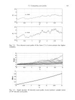
Computational example In Figure 4.2 we perform a similar experiment with
an N(0, 1) generator. Here, we took intervals in the region −4 ≤ x ≤ 4 and used
bins of width x = 0.05. (Samples that were smaller than −4 were added to the
first bin and samples that were larger than 4 were added to the last bin.) We used
M = 10
3
, 10
4
, 10
5
, 10
6
. The correct N(0, 1) density curve is superimposed in
white. We see that the density estimate improves as M increases. ♦
We now look at another technique for examining statistical aspects of data. For
agiven density function f (x) andagiven0< p < 1 define the pth quantile of f
as z( p), where

z( p)
−∞
f (x) dx = p. (4.6)
4.3 Statistical tests 37

−4 −2 0 2 4
0
0.1
0.2
0.3
0.4
0.5
1000 samples
−4 −2 0 2 4
0
0.1
0.2
0.3
0.4
0.5
10000 samples
−4 −2 0 2 4
0
0.1
0.2
0.3
0.4
0.5
100000 samples
−4 −2 0 2 4
0
0.1
0.2
0.3
0.4

0.5
1000000 samples
Fig. 4.2. Kernel density estimate for an N(0, 1) generator, with increasing num-
ber of samples. Vertical axis is N
i
/(Mx), for x = 0.05.
Given a set of data points ξ
1
,ξ
2
, ,ξ
M
,aquantile–quantile plot is produced by
(a) placing the data points in increasing order:

ξ
1
,

ξ
2
, ,

ξ
M
,
(b) plotting

ξ
k

against z(k/(M +1)).
The idea of choosing quantiles for equally spaced p = k/(M + 1) is that it
‘evens out’ the probability. Figure 4.3 illustrates the M = 9case when f (x) is the
N(0, 1) density. The upper picture emphasizes that the z(k/(M + 1)) break the
x-axis into regions that give equal area under the density curve – that is, there is
an equal chance of the random variable taking a value in each region. The lower
picture in Figure 4.3 plots the function f (x) and shows that z(k/(M + 1)) are the
points on the x-axis that correspond to equal increments along the y-axis. The idea
is that, for large M,ifthe quantile–quantile plot produces points that lie approxi-
mately on a straight line of unit slope, then we may conclude that the data points
‘look as though’ they were drawn from a distribution corresponding to f (x).To
justify this, if we divide the x-axis into M bins where x is in the kth bin if it is
closest to z(k/(M + 1)), then, having evened out the probability, we would expect
roughly one ξ
i
value in each bin. So the smallest data point,

ξ
1
, should be close
to z(1/(M + 1)), the second smallest,

ξ
2
, should be close to z(2/(M + 1)), and
so on.
Computational example Figure 4.4 tests the quantile–quantile idea. Here we
took M = 100 samples from N(0, 1) and U(0, 1) random number generators.
38 Computer simulation
−5

−4 −3 −2 −1
0 1 2 3 4 5
0
0.1
0.2
0.3
0.4
0.5
f
(
x
)
−5 −4 −3 −2 −1 0 1 2 3 4 5
0
0.2
0.4
0.6
0.8
1
N
(
x
)
Fig. 4.3. Asterisks on the x-axis mark the quantiles z(k/(M + 1)) in (4.6) for an
N(0, 1) distribution using M = 9. Upper picture: the quantiles break the x-axis
into regions where f (x) has equal area. Lower picture: equivalently, the quantiles
break the x-axis into regions where N(x) has equal increments.
Each data set was plotted against the N(0, 1) and U(0, 1) quantiles. A reference
line of unit slope is added to each plot. As expected, the data set matches well
with the ‘correct’ quantiles and very poorly with the ‘incorrect’ quantiles. ♦

Computational example In Figures 4.5 and 4.6 we use the techniques intro-
duced above to show the remarkable power of the Central Limit Theorem. Here,
we generated sets of U(0, 1) samples {ξ
i
}
n
i=1
, with n = 10
3
. These were com-
bined to give samples of the form

n
i=1
ξ
i
− nµ
σ
√
n
, (4.7)
where µ =
1
2
and σ
2
=
1
12
.Werepeated this M = 10

4
times. These M data
points were then used to obtain a kernel density estimate. In Figure 4.5 we
used bins of width x = 0.5 over [−4, 4] and plotted N
i
/(Mx) against x
i
,
as described for Figure 4.1. Here we have used a histogram,orbar graph,so
each rectangle is centred at an x
i
and has height N
i
/(Mx). The N(0, 1) den-
sity curve is superimposed as a dashed line. Figure 4.6 gives the corresponding
quantile–quantile plot. The figures confirm that even though each ξ
i
is nothing
like normal, the scaled sum (

n
i=1
ξ
i
− nµ)/(σ
√
n) is very close to N(0, 1). ♦
4.3 Statistical tests 39
−5 0 5
−5

0
5
N(0,1) samples and N(0,1) quantiles
−5 0 5
−5
0
5
N(0,1) samples and U(0,1) quantiles
−5 0 5
−5
0
5
U(0,1) samples and N(0,1) quantiles
−1 0 1 2
−1
−0.5
0
0.5
1
1.5
2
U(0,1) samples and U(0,1) quantiles
Fig. 4.4. Quantile–quantile plots using M = 100 samples. Ordered samples

ξ
1
,

ξ
2

, ,

ξ
M
on the x-axis against quantiles z(k/(M +1)) on the y-axis. Pictures
show the four possible combinations arising from N(0, 1) or U(0, 1) random num-
ber samples against N(0, 1) or U(0, 1) quantiles.
−5 −4 −3 −2 −1 0 1 2 3 4 5
0
0.05
0.1
0.15
0.2
0.25
0.3
0.35
0.4
N(0,1) density
Sample data
Fig. 4.5. Kernel density estimate for samples of the form (4.7), with N(0, 1)
density superimposed.
40 Computer simulation
−6 −4 −2 0 2 4 6
−5
−4
−3
−2
−1
0
1

2
3
4
5
Fig. 4.6. Quantile–quantile plot for samples of the form (4.7) against N(0, 1)
quantiles.
4.4 Notes and references
Much more about the theory and practice of designing and implementing computer
simulation experiments can be found in (Morgan, 2000) and (Ripley, 1987). In
particular, those references mention rules of thumb for choosing the bin width as a
function of the sample size in kernel density estimation.
The pLab website, which lives at gives informa-
tion on random number generation, and has links to free software in a variety of
computing languages.
Avery readable essay on pseudo-random number generation can be found in
(Nahin, 2000). That book also contains some wonderful probability-based prob-
lems, with accompanying MATLAB programs.
Cleve’s Corner articles ‘Normal behavior’, spring 2001, and ‘Random
Thoughts’, fall 1995, which are downloadable from www.mathworks.com/
company/newsletter/clevescorner/cleve
-
toc.shtml are informative musings on
MATLAB’s pseudo-random number generators.
As an alternative to ‘pseudo-’, it is possible to buy ‘true’ random numbers that
are generated from physical devices. For example, one approach is to record decay
times from a radioactive material. The readable article ‘Hardware random number
generators’, by Robert Davies, can be found at www.robertnz.net/hwrng.htm.
4.5 Program of Chapter 4 and walkthrough 41
EXERCISES
4.1.  Some scientific computing packages offer a black-box routine to evaluate

the error function, erf, defined by
erf(x) :=
2
√
π

x
0
e
−t
2
dt. (4.8)
Show that the N(0, 1) distribution function N(x) in (3.18) can be evaluated
as
N(x) =
1 + erf

x/
√
2

2
. (4.9)
4.2.  Show that samples from the exponential distribution with parameter λ,as
described in Exercise 3.4, may be generated as −(log(ξ
i
))/λ, where the {ξ
i
}
are U(0, 1) samples.

4.3.  Show that the quantile z( p) in (4.6) for the N(0, 1) distribution function
N(x) can be written as
z( p) =
√
2 erfinv(2 p − 1).
Here, erfinv is the inverse error function; so erfinv(x) = y means erf(y) = x,
where erf is defined in (4.8).
4.4.  In the case where f (x) is the density for the exponential distribution with
parameter λ = 1, as described in Exercise 3.4, show that the quantile z( p)
in (4.6) satisfies z( p) =−log(1 − p).
4.5 Program of Chapter 4 and walkthrough
In ch04,listed in Figure 4.7, we repeat the type of computation that produced Figure 4.5. Here, we
use samples ξ
i
in (4.7) that are the exponential of the square root of U(0, 1) samples. It follows from
Exercise 21.2 that we should take µ = 2 and σ =

(e
2
− 7)/2.
The line colormap([0.5 0.5 0.5]) sets the greyscale for the histogram; [0 0 0] is black and
[111]is white. We then use rand(’state’,100) to set the seed for the uniform pseudo-random
number generator, as described in the footnote of Section 4.2. After specifying n, M, mu and sigma,
and initializing S to an array of zeros, we perform the main task in a single for loop. The command
rand(n,1) creates an array of n values from the U(0, 1) pseudo-random number generator. We then
apply sqrt to take the square root of each entry, exp to exponentiate and sum to add up the result. In
other words
sum(exp(sqrt(rand(n,1))))
corresponds to a sample of
n


i=1
e
√
ξ
i
,
42 Computer simulation
%CH04 Program for Chapter 4
%
% Histogram illustration of Central Limit Theorem
clf
colormap([0.5 0.5 0.5])
rand(’state’,100)
n= 5e+2;
M=1e+4;
mu=2;
sigma = sqrt(0.5*(exp(2)-7));
S=zeros(M,1);
for k = 1:M
S(k) = (sum(exp(sqrt(rand(n,1)))) - n*mu)/(sigma*sqrt(n));
end
%%%%%%%%%%%%%%%% Histogram %%%%%%%%%%%%%%%%%%%
dx = 0.5;
centers = [-4:dx:4];
N=hist(S,centers);
bar(centers,N/(M*dx))
hold on
x=linspace(-4,4,100);
y=exp(-0.5*x.ˆ2)/sqrt(2*pi);

plot(x,y,’r–’,’Linewidth’,4)
legend(’N(0,1) density’,’Sample data’)
grid on
Fig. 4.7. Program of Chapter 4: ch04.m.
so overall, S(k) stores a sample of

n
i=1
e
√
ξ
i
− nµ
σ
√
n
.
The line N=hist(S,centers); creates a one-dimensional array N, whose ith entry records the
number of values in S lying in the ith bin. Here, a point is mapped to the ith bin if its closest value
in centers is centers(i). The command bar(centers,N/(M*dx)) then draws a bar graph, or
histogram, using this information. (We scale by M*dx so that the area of the histograph adds up to
one.)
Because we issued the command hold on, the second plot, a dashed line for the exact density
curve, adds to, rather than replaces, the first.