An Introduction to Financial Option Valuation: Mathematics, Stochastics and Computation_4 ppt

4.5 Program of Chapter 4 and walkthrough 43
PROGRAMMING EXERCISES
P4.1. Adapt ch04.m to the case where ξ
i
in (4.7) are from the exponential distri-
bution with parameter λ = 1. [Hint: make use of Exercise 3.4 and Exercise 4.2.]
P4.2. Adapt
ch04.m so that it produces a quantile–quantile plot, as in Figure 4.6.
(Note that the program of Chapter 5 shows how such a plot may be generated.)
Quotes
In 1955, before computers were so common,
the RAND Corporation published a book entitled A Million Random Digits.
It was used in selecting random trials for experimental designs and simulations
(and perhaps as bedtime reading for insomniacs?).
It was soon realized, however, that if everyone always started on page one,
then all trials and simulations by all the book’s users would depend upon the quirks of
the same random sequence.
This generated much debate
on how to select a random starting point in the table of random numbers.
MICHAEL T. HEATH (Heath, 2002)
The first thing needed for a stochastic simulation is a source of randomness.
This is often taken for granted but is of fundamental importance.
Regrettably many of the so-called random functions supplied with the most
widespread computers
are far from random,
and many simulation studies have been invalidated as a consequence.
BRIAN D. RIPLEY (Ripley, 1997)
Here is an interesting number:
0.950 129 285 147 18.
This is the first number produced by the MATLAB random number generator with its
default settings.

Start up a fresh MATLAB, set format long, type rand,
and it’s the number you get.
If all MATLAB users, all around the world, on all different computers,
keep getting this same number, is it really ‘random’?
No, it isn’t.
Computers are (in principle) deterministic machines
and should not exhibit random behavior.
If your computer doesn’t access some external device,
like a gamma ray counter or a clock,
then it must really be computing pseudorandom numbers.
CLEVE B. MOLER AND KATHRYN A. MOLER,inNumerical Computing with
MATLAB,
see www.mathworks.com/moler/

5
Asset price movement
OUTLINE
• efficient market hypothesis
• examples of real asset data
• tests for i.i.d. and normality
• assumptions for the model
5.1 Motivation
In order to value an option, we must develop a mathematical description of how
the underlying asset behaves. This chapter gives examples of real stock market
data and performs some basic statistical tests. The tests pave the way for the math-
ematical description that we introduce in the next chapter, but are definitely not
intended to form an exhaustive justification of the model. We begin with an out-
line of a key hypothesis, and finish by listing some of the assumptions that will go
into our analysis.
5.2 Efficient market hypothesis

The price of an asset is, of course, a measure of investors’ confidence, and, as
such, is strongly dependent upon news, rumours, speculation, and so on. Although
an oversimplification, it is reasonable to assume that the market responds instanta-
neously to external influences, and hence:
the current asset price reflects all past information.
This simple conclusion is known as the (weak form of the) efficient market hy-
pothesis. Under this hypothesis, if we want to predict the asset price at some future
time, knowing the complete history of the asset price gives no advantage over
just knowing its current price – there is no edge to be gained from ‘reading the
charts.’
45
46 Asset price movement
Jan Feb Mar Apr May Jun Jul Aug Sep
80
85
90
95
100
105
110
115
120
Price
IBM daily
Fig. 5.1. Daily IBM share price from January to September 2001.
From a modelling point of view, if we take on board the efficient market hypoth-
esis, then an equation to describe the evolution of the asset from time t to t + t
need involve the asset price only at time t and not at any earlier times.
5.3 Asset price data
In Figure 5.1 we plot the daily IBM share prices from January to the end of

September 2001. These are the close-of-trading prices; that is, the price at the last
transaction made in each trading day. In the traditional manner, we have ‘joined
the dots’ so that successive data points are linked by straight lines. Figure 5.2
gives the corresponding weekly IBM share prices from January 1998 to December
2001. There are 184 data points in Figure 5.1 and 209 in Figure 5.2. Although cov-
ering different timescales, both pictures display the same qualitative ‘jaggedness’.
This type of up/down uncertainty is familiar to anybody who has seen stock market
data displayed in graphical form.
To examine this data, it is reasonable to treat it on the same level as the output
from a pseudo-random number generator and test whether it has any statistical
properties. In Figure 5.3 we give the results of such a test. The upper pictures
involve the daily returns,
r
daily
i
:=
S(t
i+1
) − S(t
i
)
S(t
i
)
,
5.3 Asset price data 47
1998 1999 2000 2001
40
50
60

70
80
90
100
110
120
130
140
Price
IBM weekly
Fig. 5.2. Weekly IBM share price from January 1998 to December 2001.
−5 0 5
0
0.1
0.2
0.3
0.4
IBM Daily
Histogram
−5
0 5
0
0.5
1
Cumulative Density
−5
0 5
−4
−2
0

2
4
Quantiles
−5
0 5
0
0.1
0.2
0.3
0.4
IBM Weekly
−5 0 5
0
0.5
1
−5
0 5
−4
−2
0
2
4
−5
0 5
0
0.1
0.2
0.3
0.4
Rand. Num. Gen.

−5 0 5
0
0.5
1
−5 0 5
−4
−2
0
2
4
−
Fig. 5.3. Statistical tests of IBM share price data. Upper: daily. Middle: weekly.
Lower: N(0, 1) samples for comparison.
48 Asset price movement
where S(t
i
) and S(t
i+1
) are the asset prices on successive days, as used in
Figure 5.1. These daily returns were normalized to

r
daily
i
:=
r
daily
i
− µ
σ

,
where µ and σ
2
are the computed sample mean and sample variance, defined
in (4.1) and (4.2), respectively. If the daily return data looks like i.i.d. sam-
ples from a normal distribution, then

r
daily
i
will look like i.i.d. N(0, 1) samples.
The upper left picture in Figure 5.3 gives a kernel density estimate for the

r
daily
i
data in the form of a histogram, with the N(0, 1) density curve (3.15) superim-
posed as a dashed line. To estimate the corresponding distribution function, we
may use a cumulative sum histogram, where in each bin we record the proportion
of samples that fall in that bin, or in a bin to the left. This produces the histogram
in the middle picture. The N(0, 1) distribution function (3.18) is superimposed as
a dashed line. Finally, in the upper right picture we give a quantile–quantile plot,
as described in Chapter 4, using N(0, 1) quantiles. The three middle pictures in
Figure 5.3 present the same results for the normalized weekly returns, using the
data from Figure 5.2. As a basis for comparison, the lower pictures give the output
that arises when 200 points from an N(0, 1) pseudo-random number generator are
subjected to the same scrutiny.
Overall, Figure 5.3 suggests that the daily and weekly asset returns behave in a
similar manner to normally distributed i.i.d. samples. The quantile–quantile plots,
which are the most revealing, possibly indicate that the match is least accurate

at the extremes of the range – this fat tail behaviour will be mentioned again in
Section 7.4.
As a final point, we remark that since the daily and weekly returns are quite
small, the approximation log(1 + x) ≈ x gives
log

S(t
i+1
)
S(t
i
)

= log

1 +
S(t
i+1
) − S(t
i
)
S(t
i
)

≈
S(t
i+1
) − S(t
i

)
S(t
i
)
(5.1)
and hence we would see essentially the same pictures as those in Figure 5.3 if we
replaced the returns with the log ratios, log
(
S(t
i+1
)/S(t
i
)
)
.
5.4 Assumptions
In the next chapter we develop a mathematical description of the asset price move-
ment that is intended to capture the broad features that are observed in practice.
Before we do that, we take the opportunity to list some of the assumptions that will
be made in the subsequent analysis.
5.5 Notes and references 49
• The asset price may take any non-negative value.
• Buying and selling an asset may take place at any time 0 ≤ t ≤ T .
• It is possible to buy and sell any amount of the asset.
• The bid–ask spread is zero – the price for buying equals the price for selling.
• There are no transaction costs.
• There are no dividends or stock splits.
• Short selling is allowed – it is possible to hold a negative amount of the asset.
• There is a single, constant, risk-free interest rate that applies to any amount of money
borrowed from or deposited in a bank.

5.5 Notes and references
The efficient market hypothesis is at best an approximation to reality. A classic text
that espouses the hypothesis is (Malkiel, 1990). A more recent book that analyses
vast amounts of stock market data and casts severe doubt on the efficient market
hypothesis is (Lo and MacKinlay, 1999). It is important to keep in mind, however,
that it is a big leap to go from
(a) claiming that the current asset price movement is somehow correlated with historical
asset price data, to
(b) developing a method that can make these correlations sufficiently explicit to be of use
for prediction.
Bass (Bass, 1999) describes what seems to be one of the few successful, systematic
attempts in this direction. The topic is mentioned further in Section 7.4.
The data used in Figures 5.1–5.3 was downloaded from the Yahoo! Fi-
nance website at http://finance.yahoo.com/ and processed using MATLAB code
based on the tools developed by Petter Wiberg at www.maths.warwick.ac.uk/
wiberg/MathFinance/.
It is worth emphasizing that the tests in Section 5.3 were designed solely for the
purpose of illustration. There are many practical issues to address before a serious
statistical analysis of stock market data can be performed. Most notably:
• There may be missing data if no trading took place between times t
i
and t
i+1
.
• For many data sets, each price may correspond to either a buy or a sell – there is an
in-built noise level at the order of the bid–ask spread.
• The data may require adjustments to account for dividends and stock splits.
• When determining the time interval, t
i+1
− t

i
, between price data, a decision must be
made about whether to keep the clock running when the stock market has closed. Does
Friday night to Monday morning count as 2
1
2
days, or zero days?
• Foranasset that is not heavily traded, the time of the last trade may vary considerably
from day to day. Consequently, daily closing prices, which pertain to the final trade for
each day, may not relate to equally spaced samples in time.
50 Asset price movement
The book (Lo and MacKinlay, 1999) is a good source of practical information for
stock market data analysis.
Many exchanges have informative websites, including the American Stock
Exchange: www.amex.com/, the Chicago Board Options Exchange: www.
cboe.com/Home/, the London Stock Exchange: www.londonstockexchange.
com/, the New York Stock Exchange: www.nyse.com/.
EXERCISES
5.1.  Consider the following quote from Eugene Fama, who was Myron
Scholes’ thesis adviser, which can be found in (Lowenstein, 2001, page 71).
If the population of price changes is strictly normal, on the average for any stock
anobservation more than five standard deviations from the mean should be ob-
served about once every 7000 years. In fact such observations seem to occur about
once every three to four years.
Given that for X ∼ N(µ, σ
2
), P(|X − µ| > 5σ) = 5.733 × 10
−7
, deduce
how many observations per year Fama is implicitly assuming to be made.

5.2. Complete the following stock market report in an apt and amusing manner.
• Knives fell sharply.
• Guacamole dipped.
• Toilet tissue bottomed out
5.6 Program of Chapter 5 and walkthrough
The program ch05 shows one way to compute a quantile–quantile plot, as seen in Figures 4.4, 4.6 and
5.3. It is listed in Figure 5.4. We use MATLAB’s N(0, 1) pseudo-random number generator, randn.
The line samples = randn(M,1), assigns M such samples to the array samples.Wethen use
ssort = sort(sample),tocreate an array ssort containing the elements of samples, rearranged
into ascending order. The line pvals = [1:M]/(M+1), then sets up equally spaced points 1/(M +
1), 2/(M + 1), 3/(M + 1), ,M/(M + 1) and zvals = sqrt(2)*erfinv(2*pvals-1); com-
putes the required quantiles, as described in Exercise 4.3. We then plot the ordered samples against
the quantiles and superimpose a reference line of slope one.
PROGRAMMING EXERCISES
P5.1. Use the cumulative sum function cumsum and the bar graph function bar to
produce a cumulative density plot from
ch05.m,asinthe lower middle picture of
Figure 5.3.
P5.2. Use the code at
www.maths.warwick.ac.uk/wiberg/MathFinance/ to
manipulate and display real stock market data.
5.6 Program of Chapter 5 and walkthrough 51
%CH05 Program for Chapter 5
%
% Illustrates quantile plot
clf
randn(’state’,100)
M=200;
samples = randn(M,1);
ssort = sort(samples);

pvals = [1:M]/(M+1);
zvals = sqrt(2)*erfinv(2*pvals-1);
plot(ssort,zvals,’rx’)
hold on
xlim = max(abs(zvals))+1;
plot([-xlim, xlim],[-xlim,xlim],’g–’) % Reference of slope 1
title(’N(0,1) quantile-quantile plot’)
grid on
Fig. 5.4. Program of Chapter 5: ch05.m.
Quotes
A battle rages between those who say the financial markets
are theoretically impossible to beat and those who say,
‘Hey, look at me, I’m a billionaire.’
On one side are the Nobel laureates,
ensconced in the University of Chicago Business School,
who are renowned for developing equations describing ‘efficient’,
that is, unbeatable, markets.
On the other side are the speculators who beat them year in, year out
with techniques ‘proven’ not to work.
THOMAS A. BASS (Bass, 1999)
Who’d have imagined that our largest single equity underwriting
would coincide with the largest drop in history in the stock market?
Then, who’d have imagined that our first big junk bond deal
would coincide with the crash of the junk bond market?
It was striking how little control we had of events,
particularly in view of how assiduously
we cultivated the appearance of being in charge
by smoking big cigars and saying **** all the time.
MICHAEL LEWIS (Lewis, 1989)
An incident of ‘fat finger syndrome’ – inadvertently pressing the wrong button

on a computer keyboard – landed an American investment bank
52 Asset price movement
with multimillion pound losses yesterday
and is expected to cost the young city trader involved his job.
The deal amounted to £300m rather than £3m
and flashed across stock market screens just as the stock market was about to close,
causing a precipitous fall in the Footsie, the barometer of British corporate health.
Slip of the finger that cost city dearly, the Guardian,16May 2001
The traditional view in economics
is that financial agents are completely rational with perfect foresight.
Markets are always in equilibrium,
which in economics means that trading always occurs
at a price that conforms to everyone’s expectations of the future.
Markets are efficient, which means that there are no patterns in prices
that can be forecast based on a given information set.
The only possible changes in price are random,
driven by unforecastable external information.
Profits occur only by chance.
In recent years this view is eroding.
J . DOYNE FARMER (Farmer, 1999)
6
Asset price model: Part I
OUTLINE
• discrete asset model
• continuous asset model
• lognormal distribution
• confidence intervals
6.1 Motivation
Our aim in this chapter is to motivate and derive the classic model for asset price
behaviour. We do this in a heuristic manner, making clear the assumptions that are

being made and keeping in mind that the model will be used as the basis for an
option valuation theory.
Given the asset price S
0
at time t = 0, our objective is to come up with a process
that describes the asset price S(t) for all times 0 ≤ t ≤ T . Due to the unpredictable
nature of assset price movements, S(t) will be a random variable for each t. Al-
though asset prices are typically rounded to one or two decimal places, we assume
here that an asset may have any price ≥ 0.
Our approach is to set up an expression for the relative change over an inter-
val of time δt and then let δt → 0inorder to get an expression that is valid for
continuous t.
6.2 Discrete asset model
As a starting point for our model we note from Exercise 2.2 that the change in the
value of a risk-free investment over a small time interval δt can be modelled as
D(t + δt) = D(t) +rδtD(t), (6.1)
where r is the interest rate. In order to account for the typical, unpredictable
changes in asset price, we will add a random element to this equation. We saw
53
54 Asset price model: Part I
in Chapter 5 that the efficient market hypothesis says that the current asset price
reflects all the information known to investors, and hence any change in the price
is due to new information. We may build this into our model by adding a ran-
dom ‘fluctuation’ increment to the interest rate equation and making these incre-
ments independent for different subintervals. To make this precise, let t
i
= iδt,
so that asset prices are to be determined at discrete points {t
i
}.(We will then

let δt → 0toget an asset price model over 0 ≤ t ≤ T .) Our discrete-time model
is
S(t
i+1
) = S(t
i
) + µδtS(t
i
) + σ
√
δtY
i
S(t
i
), (6.2)
where
• µ is a constant parameter. (Typically µ>0, so that µδtS(t
i
) represents a general up-
ward drift of the asset price. The parameter µ plays the same role as the interest rate r
in (6.1).)
• σ ≥ 0isaconstant parameter that determines the strength of the random fluctuations.
• Y
0
, Y
1
, Y
2
, are i.i.d. N(0, 1).
It is worth emphasizing a few points.

(i) Since a N(0, 1) random variable is symmetric about the origin, the fluctuation factor
σ
√
δtY
i
is equally likely to be positive or negative, and the probability that it lies in
an interval [a, b]isthe same as the probability that it lies in the interval [−b, −a].
(ii) The presence of the factor
√
δt (rather than some other power of δt) turns out to be
necessary in order for a sensible continuous-time limit to exist. Exercise 6.1 follows
this through.
(iii) The choice of a normal distribution for Y
i
is not arbitrary – because of the Central
Limit Theorem, we would arrive at the same continuous-time model for S(t) if we
just assumed that {Y
i
}
i≥0
were i.i.d. with zero mean and unit variance. Exercise 6.2
asks you to confirm this.
The parameter µ in (6.2) is usually called the drift and σ is called the volatility.
The model is statistically the same if σ is replaced by −σ , see Exercise 6.3. Con-
vention dictates that σ is taken to be ≥ 0. Typical values for σ lie between 0.05
and 0.5, that is, 5% and 50% volatility. Because we are measuring time in years,
the units of σ
2
are per annum. The drift parameter is typically between 0.01 and
0.1, but, as we will see in Chapter 8, its value turns out to be irrelevant in valuing

an option.
We point out that in the model (6.2), the returns (S(t
i+1
) − S(t
i
))/S(t
i
) form
a normal i.i.d. sequence, in line with the broad conclusions that we drew in Sec-
tion 5.3 after examining real data.
6.3 Continuous asset model 55
6.3 Continuous asset model
Suppose we consider the time interval [0, t] with t = Lδt.Weknow S(0) = S
0
and
the discrete model (6.2) gives us expressions for S(δt), S(2δt), ,S(Lδt = t).
The plan is to let δt → 0, and hence let L →∞,toget a limiting expression for
S(t).
The discrete model (6.2) says that over each δt time interval the asset price gets
multiplied by a factor 1 + µδt + σ
√
δtY
i
, and hence
S(t) = S
0
L−1

i=0


1 + µδt + σ
√
δtY
i

.
Dividing through by S
0
and taking logs gives
log

S(t)
S
0

=
L−1

i=0
log(1 + µδt + σ
√
δtY
i
). (6.3)
We are interested in the limit δt → 0, so we would like to exploit the approxima-
tion log(1 + ) ≈  − 
2
/2 + ···, for small .There is a technical issue that we
will gloss over. The quantity Y
i

in (6.2) is a random variable, not just a real num-
ber, but it can be shown that what we are about to do is justifiable because
E(Y
2
i
)
is finite. Continuing in the belief that the log expansion remains valid, we obtain
log

S(t)
S
0

≈
L−1

i=0
(µδt + σ
√
δtY
i
−
1
2
σ
2
δtY
2
i
), (6.4)

where we have ignored terms that involve the power δt
3/2
or higher. Exercise 6.4
asks you to show that
E

µδt + σ
√
δtY
i
−
1
2
σ
2
δtY
2
i

= µδt −
1
2
σ
2
δt (6.5)
and
var

µδt + σ
√

δtY
i
−
1
2
σ
2
δtY
2
i

= σ
2
δt + higher powers of δt. (6.6)
Now, insight from the Central Limit Theorem suggests that log(S(t)/S
0
) in (6.4)
will behave like a normal random variable with mean L(µδt −
1
2
σ
2
δt) =(µ −
1
2
σ
2
)t
and variance Lσ
2

δt = σ
2
t, that is, approximately,
log

S(t)
S
0

∼ N

(µ −
1
2
σ
2
)t,σ
2
t

. (6.7)
56 Asset price model: Part I
Based on these arguments, our limiting continuous-time expression for the asset
price at time t becomes
S(t) = S
0
e
(µ−
1
2

σ
2
)t+σ
√
tZ
, where Z ∼ N(0, 1). (6.8)
In this derivation there was nothing special about starting at time zero – we can
equally well argue that the asset price evolves from time t = t
1
to t = t
2
, where
t
2
> t
1
, according to
log

S(t
2
)
S(t
1
)

∼ N

(µ −
1

2
σ
2
)(t
2
− t
1
), σ
2
(t
2
− t
1
)

.
Akey point is that across non-overlapping time intervals, the normal random vari-
ables that describe these changes will be independent. This follows because the
Y
i
in (6.2) are i.i.d. Hence, for t
3
> t
2
> t
1
we have
log

S(t

3
)
S(t
2
)

∼ N

(µ −
1
2
σ
2
)(t
3
− t
2
), σ
2
(t
3
− t
2
)

,
and is independent of log

S(t
2

)
S(t
1
)

.
So we can describe the evolution of the asset over any sequence of time points
0 = t
0
< t
1
< t
2
< t
3
< ···< t
M
by
S(t
i+1
) = S(t
i
)e
(µ−
1
2
σ
2
)(t
i+1

−t
i
)+σ
√
t
i+1
−t
i
Z
i
, for i.i.d. Z
i
∼ N(0, 1). (6.9)
6.4 Lognormal distribution
A random variable S(t) of the form (6.8) has a so-called lognormal distribution;
that is, its log is normally distributed. Note from (6.8) that since S
0
> 0, S(t) is
guaranteed to be positive at any time; we have
P(S(t)>0) = 1, for any t > 0. So
S(t) takes values in (0, ∞). The corresponding density function for S(t) is
f (x) =
exp

−(log(x /S
0
) −(µ−σ
2
/2)t)
2

2σ
2
t

xσ
√
2πt
, for x > 0, (6.10)
with f (x) = 0, for x ≤ 0, see Exercise 6.5.
The expected value, second moment, and variance of S(t) with this model turn
out to be
E(S(t)) = S
0
e
µt
, (6.11)
E(S(t)
2
) = S
2
0
e
(2µ+σ
2
)t
, (6.12)
var(S(t)) = S
2
0
e

2µt
(e
σ
2
t
− 1), (6.13)
see Exercise 6.6.
6.5 Features of the asset model 57
0 0.5 1 1.5 2 2.5 3 3.5 4
0
0.5
1
1.5
t
=1
f
(
x
)
0 0.5 1 1.5 2 2.5 343.5
0
0.5
1
1.5
t
=3
f
(
x
)

σ = 0.3
σ = 0.5
σ = 0.3
σ = 0.5
σ = 0.3
σ = 0.5
σ = 0.3
σ = 0.5
σ = 0.3
σ = 0.5
Fig. 6.1. Lognormal density (6.10) for µ = 0.05, S
0
= 1, with σ = 0.3 (solid)
and σ = 0.5 (dashed). Upper picture t = 1. Lower picture t = 3.
Computational example In Figure 6.1 we set S
0
= 1 and µ = 0.05, and plot
the lognormal density function (6.10) for σ = 0.3 and σ = 0.5. The upper pic-
ture is for t = 1 and the lower picture for t = 3. Note that the density is skewed –
it has no vertical axis of symmetry. We know from (6.13) that the variance of S(t)
grows with t, and this is clear from the figure – the density function spreads out
when t increases. The mean of S(t) also grows with t, from (6.11), although this
is less obvious in the figure. ♦
We are deliberately avoiding the direct use of stochastic calculus in this book.
However, it is worth mentioning that the process S(t) defined by (6.9) can be
regarded as the solution of a stochastic differential equation (SDE). In this context,
S(t) is often referred to as geometric Brownian motion. Section 6.6 gives some
routes into this fascinating topic.
6.5 Features of the asset model
We can get some feeling for a continuous random variable by examining its confi-

dence intervals. Suppose that
P
(
a ≤ X ≤ b
)
= 0.95.
58 Asset price model: Part I
Then we say that [a, b]isa95% confidence interval for X.Inthe case where X
is normal, there is no simple formula for the inverse of the distribution function
N (x) in (3.18), and hence confidence intervals must be computed numerically. It
is found that for X ∼ N(0, 1),
P
(
|X |≤1.96
)
= 0.95, (6.14)
see Exercise 6.7, so [−1.96, 1.96] is a 95% confidence interval for X. More gen-
erally, for X ∼ N(µ, σ
2
),wehave(Y − µ)/σ ∼ N(0, 1),so
P
(
µ − 1.96σ ≤ Y ≤ µ + 1.96σ
)
= 0.95, (6.15)
and hence [µ − 1.96σ, µ +1.96σ ]isa95% confidence interval. This result is
often expressed along the lines of
for i.i.d. normal samples, 95 times out of 100 the sample lies within two standard deviations
of the mean.
It follows from (6.7) that

[S
0
e
−1.96σ
√
t+(µ−
1
2
σ
2
)t
, S
0
e
1.96σ
√
t+(µ−
1
2
σ
2
)t
] (6.16)
is a 95% confidence interval for the asset price S(t), see Exercise 6.9. If t is small,
then
e
−1.96σ
√
t+(µ−
1

2
σ
2
)t
≈ e
−1.96σ
√
t
≈ 1 − 1.96σ
√
t
and
e
1.96σ
√
t+(µ−
1
2
σ
2
)t
≈ e
1.96σ
√
t
≈ 1 + 1.96σ
√
t.
So the confidence interval is approximately
[S

0
(1 − 1.96σ
√
t), S
0
(1 + 1.96σ
√
t)].
The width of this interval is 2S
0
1.96σ
√
t.Ifweregard the confidence interval
width as a measure of the uncertainty in the future asset price, then this result
explains the traders’ rule-of-thumb that
over small time periods, uncertainty grows like the square root of time.
Although option valuation is concerned only with the asset price over a fixed
time horizon, [0, T ], it is interesting to see what the model (6.8) predicts about
long term behaviour. Since µ and σ are positive, we see from (6.12) that
lim
t→∞
E(S(t)
2
) =∞, as t →∞.
In words, we say that the asset tends to infinity in mean square as time increases.
On the other hand, it can be shown that the (µ −
1
2
σ
2

)t term dominates the σ
√
tZ
6.6 Notes and references 59
term in (6.8), so that, with probability 1,
lim
t→∞
S(t) =

∞, if µ −
1
2
σ
2
> 0,
0, if µ −
1
2
σ
2
< 0.
(6.17)
So, according to the model, if the volatility is sufficiently large (σ
2
> 2µ) then,
with probability 1, the asset price will eventually decay to zero.
6.6 Notes and references
The asset price model that we developed is extremely widely used in mathematical
finance. The discrete version (6.2) can be regarded as a numerical approximation
to the SDE formulation. The text (Kloeden and Platen, 1992) is the classic in this

area. The expository articles (Higham, 2001; Higham and Kloeden, 2002) give
lower level entry points.
The continuous model characterized by (6.8) and (6.9) is the solution to an SDE.
Reasonably accessible SDE texts are (Gard, 1988; Mao, 1997; Øksendal, 1998),
although all require some background in stochastic processes – the text (Brze
´
zniak
and Zastawniak, 1999) is a good place for beginners to start.
The result (6.17) can be established through the Strong Law of Large Numbers,
and the µ =
1
2
σ
2
case can be dealt with by the Law of the Iterated Logarithm; these
laws are discussed, for example, in (Grimmett and Stirzaker, 2001; Kloeden and
Platen, 1999).
Although widely used, the lognormal asset price model is, of course, extremely
simplistic and open to criticism. Section 7.4 gives pointers to some of the work
that has been done on alternative models.
EXERCISES
6.1.  Consider the following variations on the discrete model:
S(t
i+1
) = S(t
i
) + µδtS(t
i
) + σδtY
i

S(t
i
),
and
S(t
i+1
) = S(t
i
) + µδtS(t
i
) + σδt
1
4
Y
i
S(t
i
).
By mimicking the heuristic derivation that led to the continuous model
(6.8), show that neither of these two variations is satisfactory.
6.2. Consider the discrete model (6.2) in the case where {Y
i
} are general
i.i.d. random variables with zero mean and unit variance (i.e., not neces-
sarily normal). Assume also that
E(Y
3
i
) and E(Y
4

i
) are finite. Mimic the
60 Asset price model: Part I
heuristic derivation that led to (6.8) and show that the same continuous
model arises.
6.3.  Explain why the model (6.2) is ‘statistically the same if σ is replaced by
−σ ’.
6.4.  Verify (6.5) and (6.6). [Hint: use Exercise 3.7.]
6.5.  Show that S(t) in (6.8) has density function (6.10). [Hint: use the
characterization
P(a ≤ S(t) ≤ b) =

b
a
f (x) dx from (3.3).]
6.6. Using (3.8), show that (6.11), (6.12) and (6.13) follow from (6.10).
6.7.  Let α be the number such that
P
(
|Z |≤α
)
= 0.95, where Z ∼ N(0, 1).
Recalling that N (·) denotes the N(0, 1) distribution function, show that α
satisfies
N (−α) =
0.05
2
.
After referring to Exercise 13.3, show that α satisfies α =
√

2 erfinv
(0.95)
.Typing this into MATLAB gives α = 1.9600 (to 4 decimal
places).
6.8.  Given that
P
(
|Z |≤2.58
)
= 0.99, for Z ∼ N(0, 1), show how (6.14)
changes when a 99% confidence interval is required.
6.9.  Show from (6.7) that (6.16) gives a 95% confidence interval for the asset
price S(t).
6.10.  Using Exercise 6.8, derive a 99% confidence interval for the asset price
S(t). Does the traders’ rule-of-thumb still apply?
6.7 Program of Chapter 6 and walkthrough
In ch06, listed in Figure 6.2, we plot the lognormal density function for two different σ values.
The resulting picture is similar to those in Figure 6.1. The array y1 stores the value of the density
function at equally spaced points in x for the first set of parameter values: t=1, S=1, mu = 0.05
and sigma = 0.3.Weplot the curve as a red dashed line. The computation is then repeated with
sigma = 0.5 and a blue dotted curve is drawn.
PROGRAMMING EXERCISES
P6.1. Adapt ch06 to give a waterfall plot illustrating how the lognormal density
function varies with σ for fixed t = 1.
P6.2. Repeat programming exercise P6.1 for t varying and σ fixed at 1.
6.7 Program of Chapter 6 and walkthrough 61
%CH06 Program for Chapter 6
%
% Plots lognormal density function.
clf

x=linspace(.01,4,500);
t=1;S=1;mu=0.05;
sigma = 0.3;
tempa = ((log(x/S) - (mu-0.5*sigmaˆ2)*t).ˆ2)/(2*t*sigmaˆ2);
tempb = x*sigma*sqrt(2*pi*t);
y1 = exp(-tempa)./tempb;
plot(x,y1,’r-’)
ylim([0 1.5])
hold on
sigma = 0.5;
tempa = ((log(x/S) - (mu-0.5*sigmaˆ2)*t).ˆ2)/(2*t*sigmaˆ2);
tempb = x*sigma*sqrt(2*pi*t);
y2 = exp(-tempa)./tempb;
plot(x,y2,’b:’)
legend(’\sigma = 0.3’,’\sigma = 0.5’,1)
title(’Lognormal density,t=1,S=1, \mu = 0.05’)
xlabel(’x’), ylabel(’f(x)’)
Fig. 6.2. Program of Chapter 6: ch06.m.
Quotes
The authors emphasize that,
as even the most cursory examination of the historical record reveals,
‘geometric Brownian motion’ is at best a first approximation
to the actual movements of the price of any real stock or collection of stocks.
Even their assumption that the governing processes are stochastic – rather than
examples of deterministic chaos – may in time be disproved
by sufficiently sensitive measurement techniques.
JAMES CASE,reviewing (Mantegna and Stanley, 2000)
The Brownian motion model is extremely popular,
not primarily because of statistical evidence,
but because it is only with this model that we can determine option prices exactly.

ROBERT F. ALMGREN (Almgren, 2002)
As a graduate student at the London School of Economics
Iwas taught that stock markets were efficient.
Broadly this means that all outstanding information about companies
62 Asset price model: Part I
is built into their share prices, i.e. they are always fairly valued.
This sad fact was hammered home to students with a series of studies
demonstrating that stock-market brokers and analysts,
people with the very best information,
fared no better in their stock-market selections than a monkey
drawing a name from a hat,
or a man throwing darts at the pages of the Wall Street Journal.
The first implication of the so-called efficient markets theory is that
there is no sure way to make money in the stock market
other than trading on inside information.
Milken, and others on Wall Street, saw that this simply was not true.
The market, which may have been quick to digest earnings data,
was grossly inefficient in valuing everything from the land a company owns to the pension
fund it creates.
MICHAEL LEWIS (Lewis, 1989)
A trade takes place when the greediest buyer,
afraid that prices will run away from him,
steps up and bids a penny more.
Or the most fearful seller, afraid of getting stuck with his merchandise,
agrees to accept a penny less.
ALEXANDER ELDER (Elder, 2002)
7
Asset price model: Part II
OUTLINE
• computing discrete asset paths

• timescale invariance
• sum-of-square returns
7.1 Computing asset paths
Having derived the model, we may use (6.9) to generate computer simulations of
asset prices. Suppose we wish to simulate the evolution of S(t) at certain points
{t
i
}
K
i=0
, with 0 = t
0
< t
1
< t
2
< ···< t
K
= T.Wemay compute values {S
i
}
K
i=0
according to
S
i+1
= S
i
e
(µ−

1
2
σ
2
)(t
i+1
−t
i
)+σ
√
t
i+1
−t
i
ξ
i
, (7.1)
where each ξ
i
is a sample from a N(0, 1) pseudo-random number generator. The
resulting points (t
i
, S
i
) form a discrete asset path.
Computational example Figure 7.1 shows the results of such a simulation
with 10
3
time points equally spaced in [0, 3]. We took S
0

= 1, µ = 0.05 and
σ = 0.1. To produce the picture, we followed the usual convention of joining
the discrete data points (t
i
, S
i
) by straight lines. Overall, the resulting picture
agrees qualitatively with typical asset price plots, such as those in Figures 5.1
and 5.2. ♦
To obtain the picture in Figure 7.1 we computed a discrete, but closely spaced,
set of data points and joined them with straight lines. The picture seems to suggest
that the points lie on a continuous, but ‘jagged’, curve. This concept can be for-
malized. On the one hand it can be shown that, with probability 1, an asset path
arising from the δt → 0 limit in (6.2) will be a continuous function of t. But on
the other hand it can also be shown that, with probability 1, the path will not have
a well-defined tangent at any point.
63
64 Asset price model: Part II
0 0.5 1 1.5 2 2.5 3
0.9
1
1.1
1.2
1.3
1.4
1.5
Discrete asset path
t
i
S

i
Fig. 7.1. Discrete asset path of the form (7.1). Discrete points are joined by
straight lines to give the impression of a continuous curve.
We would also expect from the original discrete model (6.2) that increasing the
volatility parameter σ should turn up the ‘jaggedness’. The next computational
example tests for this effect.
Computational example Figure 7.2 shows asset paths computed with the same
parameters as for Figure 7.1, except that we set σ = 0.2inthe upper picture
and σ = 0.4inthe lower picture. The same psuedo-random number sequence
{ξ
i
} was used in both cases. The results confirm that the volatility parameter σ
controls the jaggedness of the path. ♦
Although individual asset paths are nonsmooth functions, we know from (6.11)
that the mean of S(t) is smooth. This is confirmed in the next computational ex-
ample.
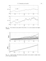
Computational example Here we take µ = 0.2 and σ = 0.3 and use 10
3
equally spaced time points over [0, 3]. We generated 10
4
such discrete paths,
starting from S
0
= 1but using different random number generator samples for
each path. The upper picture in Figure 7.3 shows the first 20 such paths. In the
lower picture we plot the sample mean: at each time point we plot the average
of the 10
4
different asset values. We see that this sample mean is indeed smooth;