An Introduction to Financial Option Valuation: Mathematics, Stochastics and Computation_5 ppt

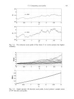
7.1 Computing asset paths 65
0 0.5 1 1.5 2 2.5 3
0.5
1
1.5
2
2.5
σ = 0.2
t
i
t
i
S
i
S
i
0 0.5 1 1.5 2 2.5 3
0.5
1
1.5
2
2.5
σ = 0.4
Fig. 7.2. Two discrete asset paths of the form (7.1). Lower picture has higher
volatility.
Fig. 7.3. Upper picture: 20 discrete asset paths. Lower picture: sample mean
of 10
4
discrete asset paths.
66 Asset price model: Part II
0 0.1 0.2 0.3 0.4 0.5 0.6 0.7 0.8 0.9 1

0
0.5
1
1.5
2
2.5
3
0 0.5 1 1.5 2 2.5 3 3.5 4 4.5 5
0
0.2
0.4
0.6
0.8
1
Fig. 7.4. Upper picture: 50 discrete asset paths over [0, T] with S
0
= 1, µ =
0.05, σ = 0.5, T = 1 and δt = 10
−2
.Lower picture: histogram for S(T ) from
10
4
such paths, with lognormal density function (6.10) superimposed.
it is visually indistinguishable from the exact mean S
0
e
µt
that we derived
in (6.11). ♦
We next give a test that confirms the lognormal behaviour of the asset model.

Computational example Here, we set S
0
= 1, µ = 0.05 and σ = 0.5, and com-
puted discrete paths over [0, T ], with T = 1. We used a uniform time spacing of
t
i+1
− t
i
= δt = 10
−2
. The upper picture in Figure 7.4 shows 50 such paths. In
the lower picture we give a kernel density estimate for the asset price at expiry.
This was computed in the manner discussed in Section 4.3, using a histogram
with 45 bins of width 0.05. The corresponding lognormal density function (6.10),
which is superimposed as a dashed line, gives a good match. ♦
7.2 Timescale invariance
The next computational example reveals a key property of the asset price model.
The jaggedness looks the same over a range of different timescales. In other
words, zooming in or out of the picture, we see the same qualitative behaviour.
We saw the same effect when we moved from daily to weekly data in Figures 5.1
and 5.2.
7.2 Timescale invariance 67
0 0.2 0.4 0.6 0.8 1
0.5
1
1.5
Asset path zoom
0 0.02 0.04 0.06 0.08 0.1
0.8
1

1.2
0 0.002 0.004 0.006 0.008 0.01
0.95
1
1.05
Fig. 7.5. The same asset path sampled at different scales. Upper picture: 100
samples over [0, 1]. Middle picture: 100 samples over [0, 0.1]. Lower picture:
100 samples over [0, 0.01].
Computational example To generate Figure 7.5, we computed a single asset
path for S
0
= 1, µ = 0.05 and σ = 0.5atequally spaced time points in [0, 1] a
distance 10
−4
apart. Using this data, we plot three pictures. Each picture shows
the path at 100 equally spaced time points.
• The upper plot shows the path at 100 equally spaced points in [0, 1].
• The middle plot shows the path at 100 equally spaced points in [0, 0.1].
• The lower plot shows the path at 100 equally spaced points in [0, 0.01]
We see that zooming in on the path in this manner does not reveal any change in
the qualitative features – the path is ‘jagged’ at all time scales. ♦
To understand why the pictures have this ‘timescale stability’ we go back to the
discrete model (6.2) and consider
• a small time interval δt,
• very small time interval

δt = δt/L, where L is a large integer. (In Figure 7.5 we used
quite a moderate value, L = 10.)
Using (6.2) to get from time t = 0tot =


δt we have
S(

δt) − S
0
= S
0
(µ

δt + σ


δtY
0
) = S
0
N(µ

δt,σ
2

δt) (7.2)
68 Asset price model: Part II
for the change in S(t). From time t = 0tot = δt, increments like this add up:
S(δt) − S
0
=
L−1

i=0


S((i + 1)

δt) − S(i

δt)

=
L−1

i=0
S(i

δt)(µ

δt + σ


δtY
i
).
Approximating
1
each S(i

δt) by S
0
and using insight from the Central Limit The-
orem suggests that
S(δt) − S

0
≈ S
0
L−1

i=0

µ

δt + σ


δtY
i

= S
0
N(µL

δt,σ
2
L

δt) = S
0
N(µδt,σ
2
δt),
which reproduces (7.2) over the longer timescale.
7.3 Sum-of-square returns

In Section 5.3 we introduced the concept of the return of an asset; this is simply
the relative price change. For small δt = t
i+1
− t
i
our original discrete model (6.2)
assumes that
S(t
i+1
) − S(t
i
)
S(t
i
)
= µδt + σ
√
δtY
i
, (7.3)
so the return is an N(µδt,σ
2
δt) random variable. Under this model we know the
statistics of the return – given any numbers a and b we can work out the probability
that the return over the next interval lies between a and b,but, of course, we cannot
predict with any certainty what actual return will be seen.
By contrast with the uncertainty of returns, we can show that the sum-of-square
returns is predictable. Suppose the interval [0, t]isdivided into a large number of
equally spaced subintervals [0, t
1

], [t
1
, t
2
], , [t
L−1
, t
L
], with t
i
= iδt and δt =
t/L. Then from (7.3) it is straightforward to show that
E


S(t
i+1
) − S(t
i
)
S(t
i
)

2

= σ
2
δt + higher powers of δt, (7.4)
and

var


S(t
i+1
) − S(t
i
)
S(t
i
)

2

= 2σ
4
δt
2
+ higher powers of δt, (7.5)
see Exercise 7.1.
Hence, using insight from the Central Limit Theorem,

L−1
i=0
((S(t
i+1
)−
S(t
i
))/S(t

i
))
2
should behave like N(Lσ
2
δt, L2σ
4
δt
2
), that is, N(σ
2
t, 2σ
4
tδt).
This random variable has a variance proportional to δt, and hence is essentially
1
Some justification for this type of approximation can be found in Section 8.2.
7.4 Notes and references 69
0 0.1 0.2 0.3 0.4 0.5
0.6
0.8
1
1.2
1.4
1.6
d
t
= 5 × 10
−3
d

t
= 5 × 10
−4
Asset paths
0 0.1 0.2 0.3 0.4 0.5
0
0.01
0.02
0.03
0.04
0.05
Sum-of-square returns
σ
2
/2 σ
2
/2σ
2
/2
0 0.1 0.2 0.3 0.4 0.5
0.8
0.9
1
1.1
Asset paths
0 0.1 0.2 0.3 0.4 0.5
0
0.01
0.02
0.03

0.04
0.05
Sum-of-square returns
σ
2
/2
Fig. 7.6. Upper pictures: asset paths. Lower pictures: running sum-of-square
returns (7.6).
constant. Thus, although the individual returns are unpredictable, the sum of the
squared returns taken over a large number of small intervals is approximately equal
to σ
2
t.
Computational example Figure 7.6 confirms the sum-of-square returns result.
We use S
0
= 1, µ = 0.05 and σ = 0.3. Ten asset paths over [0, 0.5] are shown
in the upper left plot. The paths were computed using equally spaced time points
adistance δt = 0.5/100 = 5 × 10
−3
apart, so L = 100. The lower left picture
plots the running sum-of-square returns
k

i=1

S(t
i+1
) − S(t
i

)
S(t
i
)

2
(7.6)
against t
k
for each path. The sum is seen to approximate σ
2
t
k
; the height
σ
2
/2isshown as a dotted line. The right-hand pictures repeat the experiment
with L = 10
3
,soδt = 5 × 10
−4
.Wesee that reducing δt has improved the
match. ♦
7.4 Notes and references
Our treatment of timescale invariance in Section 7.2 can be made rigorous, but the
concepts required are beyond the scope of this book. (The essence is that if W(t) is
70 Asset price model: Part II
a Brownian motion then so is W(c
2
t)/c, for any constant c > 0; see, for example,

(Brze
´
zniak and Zastawniak, 1999, Exercise 6.28) and (Brze
´
zniak and Zastawniak,
1999, Exercise 7.20), and their solutions, for details of this result and why it applies
to the asset model.)
There have been numerous attempts to develop generalizations or alternatives to
the lognormal asset price model. Many of these are motivated by the observation
that real market data has fat tails –extreme events occur more frequently than a
model based on normal random variables would predict.
One approach is to allow the volatility to be stochastic, see (Duffie, 2001; Hull,
2000; Hull and White, 1987), for example. Another is to allow the asset to undergo
‘jumps’, see (Duffie, 2001; Hull, 2000; Kwok, 1998), for example. Jump models
are especially popular for modelling assets from the utility industries, such as elec-
trical power. The article (Cyganowski et al., 2002) discusses some implementation
issues.
An alternative is to take a general, parametrized class of random variables and
fit the parameters to stock market data, see (Rogers and Zane, 1999), for example.
A completely different approach is to abandon any attempt to understand the
processes that drive asset prices (in particular to pay no heed to the efficient mar-
kethypothesis) and instead to test as many models as possible on real market data,
and use whatever works best as a predictive tool. A group of mathematical physi-
cists with expertise in chaos and nonlinear time series, led by Doyne Farmer and
Norman Packard, took up this idea. They founded The Prediction Company in
Santa Fe. The company has a website at www.predict.com/html/ introduction.html
which makes the claim that
Our technology allows us to build fully automated trading systems which can handle huge
amounts of data, react and make decisions based on that data and execute transactions
based on those decisions – all in real time. Our science allows us to build accurate and

consistent predictive models of markets and the behavior of financial instruments traded in
those markets.
The book (Bass, 1999) gives the story behind the foundation and early years of the
company and has many insights into the practical issues involved in collecting and
analysing vast amounts of financial data.
EXERCISES
7.1. Confirm the results (7.4) and (7.5).
7.2.  By analogy with the continuously compounded interest rate model, we
may define the continuously compounded rate of return for an asset over
[0, t]tobethe random variable R satisfying S(t) = S
0
e
Rt
. Using (6.8), show
that R ∼ N(µ −σ
2
/2,σ
2
/t).
7.5 Program of Chapter 7 and walkthrough 71
7.5 Program of Chapter 7 and walkthrough
The program ch07, listed in Figure 7.7, produces a plot of 50 asset paths in the style of the upper pic-
ture in Figure 7.4. Having initialized the parameters, we make use of the cumulative product function,
cumprod,toproduce an array of asset paths. Generally, given an M by L array X, cumprod(X) cre-
ates an M by L array whose (i, j) element is the product X(1,j)*X(2,j)*X(3,j)* *X(i,j).
Supplying a second argument set to 2 causes the cumulative product to be taken along the sec-
ond index – across rows rather than down columns, so cumprod(X,2) creates an M by L array
whose (i, j) element is the product X(i,1)*X(i,2)*X(i,3)* *X(i,j).Wealso supply two
arguments to the randn function: randn(M,L) produces an M by L array with elements from the
randn pseudo-random number generator.

It follows that
Svals = S*cumprod(exp((mu-0.5*sigma^2)*dt + sigma*sqrt(dt)*randn(M,L)),2);
creates an M by L array whose ith row represents a single discrete asset path, as in (6.9). The next
line
Svals = [S*ones(M,1) Svals]; % add initial asset price
adds the initial asset as a first column, so that the ith row Svals(i,1),Svals(i,2), ,
Svals(i,L+1) represents the asset path at times 0,dt,2dt,3dt, ,T.
PROGRAMMING EXERCISES
P7.1. Write a program that illustrates the timescale invariance of the asset model,
in the style of Figure 7.5.
P7.2. Use
mean and std to verify the approximations (7.4) and (7.5) for (7.3).
%CH07 Program for Chapter 7
%
% Plot discrete sample paths
randn(’state’,100)
clf
%%%%%%%%% Problem parameters %%%%%%%%%%%
S=1;mu=0.05; sigma = 0.5;L=1e2;T=1;dt=T/L; M = 50;
%%%%%%%%%%%%%%%%%%%%%%%%%%%%%%%%
tvals = [0:dt:T];
Svals = S*cumprod(exp((mu-0.5*sigmaˆ2)*dt + sigma*sqrt(dt)*randn(M,L)),2);
Svals = [S*ones(M,1) Svals]; % add initial asset price
plot(tvals,Svals)
title(’50 asset paths’)
xlabel(’t’), ylabel(’S(t)’)
Fig. 7.7. Program of Chapter 7: ch07.m.
72 Asset price model: Part II
Quotes
But as a warning,

let me note that a trader with a better model might still not be able to transform
this knowledge into money.
Finance is consistent in its ability to build good models
and consistent in its inability to make easy money.
The purpose of the model is to understand the factors
that influence and move option prices
butinthe absence of an ability to forecast these factors
the transformation into money remains non-trivial.
DILIP B. MADAN (Madan, 2001)
Evidence countering the efficient market hypothesis
comes in the form of stock market anomalies.
These are events that violate the assumption that stock returns
are randomly distributed.
They include the size effect
(big-company stocks out-perform small-company stocks or vice versa);
the January effect
(stock returns are abnormally high during the first few days of January);
the week-of-the-month effect
(the market goes up at the beginning and down at the end of the month);
and the hour-of-the-day effect
(prices drop during the first hour of trading on Monday and rise on other days).
Prices fall faster than they rise;
the market suffers from ‘roundaphobia’
(the Dow breaking ten thousand is a big deal);
and the market tends to overreact
(aggressive buying after good news is followed by nervous selling,
no matter what the news).
Finally, the efficient market hypothesis is incapable of explaining
stock market bubbles and crashes, insider trading, monopolies,
and all the other messy stuff that happens outside its perfect models.

THOMAS A. BASS (Bass, 1999)
Prices reflect intelligent behavior of rational investors and traders,
but they also reflect screaming mass hysteria.
ALEXANDER ELDER (Elder, 2002)
8
Black–Scholes PDE and formulas
OUTLINE
• sum-of-squares for asset price
• replicating portfolio
• hedging
• Black–Scholes PDE
• Black–Scholes formulas for a European call and put
8.1 Motivation
At this stage we have defined what we mean by a European call or put option on
an underlying asset and we have developed a model for the asset price movement.
We are ready to address the key question: what is an option worth? More precisely,
can we systematically determine a fair value of the option at t = 0?
The answer, of course, is yes, if we agree upon various assumptions. Although
our basic aim is to value an option at time t = 0 with asset price S(0) = S
0
,we
will look for a function V (S, t) that gives the option value for any asset price S ≥ 0
at any time 0 ≤ t ≤ T . Moreover, we assume that the option may be bought and
sold at this value in the market at any time 0 ≤ t ≤ T .Inthis setting, V (S
0
, 0) is
the required time-zero option value. We are going to assume that such a function
V (S, t) exists and is smooth in both variables, in the sense that derivatives with
respect to these variables exist. It was mentioned in Section 7.1 that S(t) is not a
smooth function of t –itisjagged, without a well-defined first derivative. However,

it is still perfectly possible for the option value V (S, t) to be smooth in S and t.
Looking ahead, Figures 11.3 and 11.4 illustrate this fundamental disparity.
Our analysis will lead us to the celebrated Black–Scholes partial differential
equation (PDE) for the function V . The approach is quite general and the PDE
is valid in particular for the cases where V (S, t) corresponds to the value of a
European call or put.
73
74 Black–Scholes PDE and formulas
The key idea in this chapter is hedging to eliminate risk.Toreinforce the idea,
and emphasize that it is a concrete tool as well as a theoretical device, the next
chapter is devoted to computational experiments that illustrate hedging in practice.
Before launching into a description of hedging, we first introduce one of the
main ingredients that goes into the analysis.
8.2 Sum-of-square increments for asset price
To make progress, we need to work on two timescales. For the rest of the chapter
we use
• a small timescale, determined by a time increment t, and
• a very small timescale, determined by a time increment δt = t/L, where L is a large
integer.
We consider some general time t ∈ [0, T ] and general asset price S(t) ≥ 0, and fo-
cus on the small time interval [t, t + t]. This is broken down into equally spaced,
very small, subintervals of length δt,giving[t
0
, t
1
], [t
1
, t
2
], , [t

L−1
, t
L
] with
t
0
= t, t
L
= t +t and, generally, t
i
= t +i δt.
We will let
δS
i
:= S(t
i+1
) − S(t
i
)
denote the change in asset price over a very small time increment. Before attempt-
ing to derive the Black–Scholes PDE, we need to establish a preliminary result
about the sum-of-square increments,

L−1
i=0
δS
2
i
.Asimilar analysis was done in
Section 7.3 for the sum-of-square returns,


L−1
i=0
(δS
i
/S(t
i
))
2
.
Returning to the discrete model (6.2) we have
δS
i
= S(t
i
)(µδt + σ
√
δtY
i
),
where the Y
i
are i.i.d. N(0, 1).So
L−1

i=0
δS
2
i
=

L−1

i=0
S(t
i
)
2
(µ
2
δt
2
+ 2µσ δt
3
2
Y
i
+ σ
2
δtY
2
i
). (8.1)
We now make this summation amenable to the Central Limit Theorem by replacing
each S(t
i
) by S(t ). This approximation, which is discussed further in the next
paragraph, gives us
L−1

i=0

δS
2
i
≈ S(t)
2
L−1

i=0
(µ
2
δt
2
+ 2µσ δt
3
2
Y
i
+ σ
2
δtY
2
i
). (8.2)
8.2 Sum-of-square increments for asset price 75
Working out the mean and variance of the random variables inside the summation
and appealing to the Central Limit Theorem suggests the approximate relation
L−1

i=0
δS

2
i
∼ S(t)
2
N(σ
2
Lδt, 2σ
4
Lδt
2
) = S(t)
2
N(σ
2
t, 2σ
4
tδt), (8.3)
see Exercise 8.1. Because δt is very small, the variance of that final expression is
tiny, leading us to conclude that the sum-of-square increments is approximately a
constant multiple of S(t)
2
:
L−1

i=0
δS
2
i
≈ S(t)
2

σ
2
t. (8.4)
The step of replacing each S(t
i
) in (8.1) by S(t) can be loosely justified as
follows. Our model (6.9) shows that
S(t
i
) = S(t)e
(µ−
1
2
σ
2
)iδt+σ
√
iδtZ
, for some Z ∼ N(0, 1).
Using e
x
≈ 1 + x for small x,wehave
S(t
i
) ≈ S(t)(1 + σ
√
iδtZ)
and since iδt ≤ Lδt = t,wemay write, loosely,
S(t
i

) − S(t) = O(
√
t).
In words, approximating each S(t
i
) by S(t) introduces an error that is roughly
proportional to
√
t.Wemay thus argue that replacing each S(t
i
) in (8.1) with
S(t) will not affect the leading term in the approximation (8.4). This is far from a
rigorous argument – Z is a random variable, not simply a real number – but it can
be shown that the overall conclusion is valid.
Computational example Although we are not in a position to prove (8.4) rigo-
rously, we can certainly illustrate the result via a computational experiment. We
may copy the way that Figure 7.6 was produced, but now computing the sum-
of-square increments, instead of the sum-of-square returns. We set S
0
= 1, µ =
0.05 and σ = 0.3. The upper left plot in Figure 8.1 shows ten discrete asset
paths over [0,t] with t = 0.5, using equally spaced points a distance δt =
t/100 = 5 × 10
−3
apart. So L = 100 and t = 0. The lower left picture plots
the running sum-of-square increments
k

i=1
δS

2
i
(8.5)
76 Black–Scholes PDE and formulas
Fig. 8.1. Upper pictures: asset paths. Lower pictures: running sum-of-square
increments (8.5).
against t
k
for each path. We see that the sum typically approximates σ
2
t =
0.045 as k approaches L. The right-hand pictures give the same information for
an example with t = 0.1andL = 1000, so δt = 10
−4
.Wesee that the quality
of the approximation (8.4) has improved. ♦
8.3 Hedging
Now, to find a fair option value, we set up a replicating portfolio of asset and cash,
that is, a combination of asset and cash that has precisely the same risk as the
option at all time. The portfolio will consist of a cash deposit D and a number A
of units of asset. We allow D and A to be functions of asset price S and time t.
The portfolio value, denoted by , thus satisfies
(S, t) = A(S, t)S + D(S, t). (8.6)
We must specify how the asset holding A(S, t) and cash deposit D(S, t) are
going to vary with S and t. Before delving into the details it is perhaps useful to
remind ourselves of some basic assumptions that are being made, all of which have
been introduced earlier:
• there are no transaction costs,
• the asset can be bought/sold in arbitrary units,
8.3 Hedging 77

• short selling is permitted,
• no dividends are paid,
• the interest rate r is constant,
• trading of the asset (and option) can take place in continuous time.
To avoid unreadably long equations we will also introduce some shorthand nota-
tion. A subscript i denotes evaluation of a function at (S(t
i
), t
i
),so
V
i
means V (S(t
i
), t
i
), 
i
means (S(t
i
), t
i
), etc.
No subscript denotes evaluation at (S(t), t ),so
V means V (S(t), t),  means (S(t), t), etc.
The symbol δ denotes the difference over a timestep of length δt,so
• δS
i
means S(t
i+1

) − S(t
i
),
• δV
i
means V (S(t
i+1
), t
i+1
) − V (S(t
i
), t
i
),
• δ
i
means (S(t
i+1
), t
i+1
) − (S(t
i
), t
i
),
• δ(V − )
i
means δV
i
− δ

i
,etc.
Our strategy for the portfolio (8.6) is to keep the amount of asset constant over
each very small timestep of length δt.Itfollows that the change in the value of the
portfolio has two sources.
(1) The asset price fluctuation. The change δS
i
produces a change A
i
δS
i
in the portfolio
value.
(2) Interest accrued on the cash deposit. Using the discrete version for convenience (see
(2.7) in Exercise 2.2), we may write this contribution to the portfolio change as rD
i
δt.
Overall,
δ
i
= A
i
δS
i
+rD
i
δt. (8.7)
Now because V is assumed to be a smooth function of S and t,aTaylor series
expansion gives
δV

i
≈
∂V
i
∂t
δt +
∂V
i
∂ S
δS
i
+
1
2
∂
2
V
i
∂ S
2
δS
2
i
. (8.8)
We have kept the δS
2
i
term in (8.8) because experience from the previous two chap-
ters suggests that it will make a contribution of size proportional to δt. Subtracting
(8.7) from (8.8) in order to compare the change in the portfolio with that in the

option value, we find
δ(V − )
i
≈

∂V
i
∂t
−rD
i

δt +

∂V
i
∂ S
− A
i

δS
i
+
1
2
∂
2
V
i
∂ S
2

δS
2
i
. (8.9)
78 Black–Scholes PDE and formulas
Our aim is to make the portfolio replicate the option, so that the difference
between them is predictable. We can eliminate the unpredictable δS
i
term from
(8.9) by setting
A
i
=
∂V
i
∂ S
, (8.10)
in which case
δ(V − )
i
≈

∂V
i
∂t
−rD
i

δt +
1

2
∂
2
V
i
∂ S
2
δS
2
i
. (8.11)
The final step in eliminating randomness is to add these differences over 0 ≤ i ≤
L − 1 and exploit (8.4), which shows that the sum of the δ S
2
i
terms is nonrandom.
Before proceeding with that final step, we pause to explain what (8.10) means
in practice. If we are able to find the required function V , then we may differ-
entiate it with respect to S in order to specify our strategy for updating the port-
folio. At the end of the step from t
i
to t
i+1
we rebalance our asset holding to
A
i+1
= ∂V
i+1
/∂ S. This may involve selling (if ∂ V
i+1

/∂ S <∂V
i
/∂ S)orbuying
(if ∂ A
i+1
/∂ S >∂A
i
/∂ S) some amount of the asset. We want to make the portfolio
self-financing, that is, beyond time t = 0wedonot want to add or remove money.
This can be achieved by using the cash account to finance the update – the money
needed for, or generated by, the asset rebalancing, is reflected by a corresponding
change from D
i
to D
i+1
. This idea of continually fine-tuning the portfolio in order
to reduce or remove risk is known as hedging.
8.4 Black–Scholes PDE
Letting (V − ) denote the change in V −  from time t to t + t, that is,
(V − ) = V (S(t + t), t +t) − (S(t + t), t + t)
−
(
V (S(t), t) − (S(t), t)
)
,
we may sum (8.11) to give
(V − ) ≈
L−1

i=0


∂V
i
∂t
−rD
i

δt +
1
2
L−1

i=0
∂
2
V
i
∂ S
2
δS
2
i
. (8.12)
On the basis that V and D are smooth functions, we will replace the arguments
S(t
i
), t
i
in ∂V
i

/∂t, D
i
and ∂
2
V
i
/∂ S
2
,byS(t), t,inasimilar manner to the approx-
imation used for (8.1). So, using Lδt = t,
(V − ) ≈

∂V
∂t
−rD

t +
1
2
∂
2
V
∂ S
2
L−1

i=0
δS
2
i

.
8.4 Black–Scholes PDE 79
Now, using (8.4), and assuming that all approximations are exact in the limit δt →
0, we may write
(V − ) =

∂V
∂t
−rD+
1
2
σ
2
S
2
∂
2
V
∂ S
2

t. (8.13)
The final leap of logic is to argue that because this change in the portfolio V − 
is nonrandom, it must equal the corresponding growth offered by the risk-free
interest rate, so
(V − ) = rt(V − ). (8.14)
This follows from the no arbitrage principle. If (V − ) > rt(V − ) then
we could make a guaranteed profit greater than that offered by the risk-free interest
rate by
(i) acquiring the portfolio V − at time t –buying the option at V in the marketplace,

and selling the portfolio  (i.e. short selling A units of asset and loaning out an amount
D of cash), and
(ii) selling the portfolio V − at time t +t.
Similarly, if (V − ) < rt(V − ) then we could make a guaranteed profit
greater than that offered by the risk-free interest rate by
(i) selling the portfolio V −  at time t – selling the option at V in the marketplace, and
buying the portfolio  (i.e. buying A units of asset and borrowing an amount D of
cash), and
(ii) buying the portfolio V −  at time t + t.
Now, combining (8.6), (8.13) and (8.14) gives
∂V
∂t
−rD+
1
2
σ
2
S
2
∂
2
V
∂ S
2
= r(V − AS − D).
Using A = ∂V /∂ S from (8.10) and rearranging, we arrive at
∂V
∂t
+
1

2
σ
2
S
2
∂
2
V
∂ S
2
+rS
∂V
∂ S
−rV = 0. (8.15)
This is the famous Black–Scholes partial differential equation (PDE). It is a rela-
tionship between V , S, t and certain partial derivatives of V .
Two points are worth raising immediately.
(1) The drift parameter µ in the asset model does not appear in the PDE.
(2) We have not yet specified what type of option is being valued. The PDE must be sat-
isfied for any option on S whose value can be expressed as some smooth function
V (S, t).
80 Black–Scholes PDE and formulas
Regarding point (2), to determine V (S, t) uniquely we must specify other condi-
tions that involve information about the particular option. As is typical with many
differential equations, these will apply somewhere along the edges of the domain
0 ≤ S,0≤ t ≤ T on which the problem is posed.
We will use C(S, t) to denote the European call option value. In this case, we
know for certain that at the expiry time, t = T , the payoff is max(S(T ) − E, 0).
This must be the value of the option at time T , otherwise an obvious arbitrage
opportunity exists. So

C(S, T ) = max(S(T ) − E, 0). (8.16)
Now if the asset price is ever zero, then it is clear from (6.9) that S(t) remains zero
for all time and hence the payoff will be zero at expiry. So, in this case, the value
of the option must be zero at all times. Hence,
C(0, t) = 0, for all 0 ≤ t ≤ T. (8.17)
Conversely, if the asset price is ever extremely large, then it is very likely to remain
extremely large and swamp the exercise price, so that,
C(S, t) ≈ S, for large S. (8.18)
The constraint (8.16) is called a final condition,asitapplies at the final time
t = T .Itismuch more common to come across initial conditions, specified at
t = 0, and we will see in Chapter 24 that the PDE is easily transformed into such
aproblem. The other constraints, (8.17) and (8.18), are known as boundary condi-
tions.
8.5 Black–Scholes formulas
Imposing (8.16), (8.17) and (8.18) on the Black–Scholes PDE (8.15) is enough to
force a unique solution to exist for the call option value. (In fact we could get away
with less boundary information, see Section 8.6.) This solution is
C(S, t) = SN(d
1
) − Ee
−r(T −t)
N (d
2
), (8.19)
where N (·) is the N(0, 1) distribution function, defined in (3.18), and
d
1
=
log(S/E) +(r +
1

2
σ
2
)(T − t)
σ
√
T − t
, (8.20)
d
2
=
log(S/E) +(r −
1
2
σ
2
)(T − t)
σ
√
T − t
. (8.21)
8.5 Black–Scholes formulas 81
We may also write
d
2
= d
1
− σ
√
T − t, (8.22)

see Exercise 8.2. The equation (8.19) displays the Black–Scholes formula for the
value of a European call. It is possible to construct the formula by solving the PDE
(8.15) under (8.16), (8.17) and (8.18). In this book, we take the easier route of
verifying directly that C(S, t) in (8.19) has the right properties. Exercise 8.3 deals
with (8.16), (8.17) and (8.18), and Section 10.4 deals with the PDE (8.15).
Having obtained a formula for a European call option value, we may exploit
put–call parity to establish the value P(S, t) of a European put option. In Sec-
tion 2.5 we derived the relation (2.2) that connects the time-zero call and put val-
ues. Letting P(S, t) denote the put value at asset price S and time t, the same
argument gives the general put–call parity relation
C(S, t) + Ee
−r(T −t)
= P(S, t) + S, (8.23)
see Exercise 8.4. Combining (8.19) and (8.23) leads to the Black–Scholes formula
for the value of a European put option,
P(S, t) = Ee
−r(T −t)
(
1 − N (d
2
)
)
+ S
(
N (d
1
) −1
)
.
Using Exercise 3.9, this may be simplified to

P(S, t) = Ee
−r(T −t)
N (−d
2
) − SN(−d
1
). (8.24)
Alternatively, we could derive final time and boundary conditions and attempt to
solve the Black–Scholes PDE. Since the payoff for a put option at time t = T is
max(E − S(T ), 0),wehave
P(S, T ) = max(E − S(T ), 0). (8.25)
If the asset price is ever zero then S(T ) = 0 and the payoff at time T will be E.To
obtain P(0, t) we discount for inflation, to get
P(0, t) = Ee
−r(T −t)
, for all 0 ≤ t ≤ T. (8.26)
Forextremely large S the payoff is almost certain to be zero, so
P(S, t) ≈ 0, for large S. (8.27)
Exercise 8.5 asks you to confirm that P(S, t) in (8.24) satisfies the conditions
(8.25)–(8.27) and in Exercise 10.7 of Chapter 10 you are set the task of showing
that it solves the Black–Scholes PDE (8.15).
Computational example For illustration, we give a simple example of evalu-
ating the Black–Scholes formulas. With t = 0, S
0
= 5, E = 4, T = 1, σ = 0.3
82 Black–Scholes PDE and formulas
and r = 0.05, we find, to four decimal places,
d
1
= 1.0605,

d
2
= 0.7605,
N (d
1
) = 0.8555,
N (d
2
) = 0.7765,
N (−d
1
) = 0.1445,
N (−d
2
) = 0.2235.
Here, we used MATLAB’s
erf function in order to evaluate N(x) – see Exer-
cise 4.1. The resulting European call and put option values are
C(5, 0) = 1.3231 and P(5, 0) = 0.1280.
The put–call parity relation (2.2) is easily confirmed. ♦
8.6 Notes and references
The two classic references for the Black–Scholes theory are the paper (Black and
Scholes, 1973) by Fischer Black and Myron S. Scholes, which derives the key
equations, and the paper (Merton, 1973) by Robert C. Merton, which adds a rig-
orous mathematical analysis. Merton and Scholes were awarded the 1997 Nobel
Prize in Economic Sciences for this work. It is widely accepted that Fischer Black,
who died in 1995, would have shared in the prize had he still been alive. Details of
the prize can be found at www.nobel.se/economics/laureates/1997/.
The accompanying press release argues that
Anew method to determine the value of derivatives stands out

among the foremost contributions to economic sciences
over the last 25 years.
The heuristic, discrete-time treatment of hedging that we used to derive the
Black–Scholes PDE was inspired by the expository article of Almgren (Almgren,
2002). Modern texts that give rigorous derivations of the Black–Scholes formula
include (Bj
¨
ork, 1998; Duffie, 2001; Karatzas and Shreve, 1998; Nielsen, 1999;
Øksendal, 1998).
It is possible to weaken the boundary conditions (8.17) and (8.18) in the Black–
Scholes PDE (8.15) without sacrificing uniqueness of the solution. Some control
on the growth of the solution as S →∞would suffice, see for example (Wilmott
et al., 1995). We will return to the issue of boundary conditions when we discuss
finite difference methods in Chapters 23 and 24.
8.7 Program of Chapter 8 and walkthrough 83
As a final comment, we note that although the time-T call value is a nonsmooth
hockey stick, (8.16), the function C(S, t) is smooth at all times 0 ≤ t < T ; this
phenomenon of ‘instant smoothing’ is typical of diffusion PDEs like (8.15).
EXERCISES
8.1.  Show that (8.2) leads to the approximate relation (8.3). [Hint: use Exer-
cise 3.7.]
8.2.  Show that (8.21) can be replaced by (8.22).
8.3. Confirm that C(S, t) in (8.19) satisfies (8.16), (8.17) and (8.18). [Hint:
to deal with (8.16), take the limit t → T
−
,todeal with (8.17) take the limit
S → 0
+
and to deal with (8.18) take the limit S →∞.]
8.4.  Use the argument in Section 2.5 to obtain the general put–call parity

relation (8.23).
8.5. Confirm that P(S, t) in (8.24) satisfies (8.25)–(8.27).
8.6.  It is intuitively obvious that call and put options are linear – the value of
two options is twice the value of one option. Show how this follows from
the Black–Scholes formulas (8.19) and (8.24).
8.7. Show that lim
E→0
C(S, t) = S in (8.19) and lim
E→0
P(S, t) = 0in
(8.24), and give a financial interpretation of the results.
8.8. Write down a PDE and final time/boundary conditions for the value
of a butterfly spread, as described in Exercise 1.3.
8.9. Verify that
V (S, t) =
e
(σ
2
−2r)(T −t)
S
is a solution of the Black–Scholes PDE (8.15). What is the practical impli-
cation of this result?
8.10. Verify that S and e
rt
are solutions of the Black–Scholes PDE (8.15)
and give an accompanying financial explanation.
8.11. Consider the problem posed in Exercise 2.6 of finding a fair value for
a forward contract. Use Exercise 8.7 above to confirm that F = S(0)e
rT
.

8.7 Program of Chapter 8 and walkthrough
Unlike the previous seven cases, our code for this chapter, which is listed in Figure 8.2, is a MATLAB
function. This means that it must be supplied with input arguments and it will return output argu-
ments.The input arguments S,E,r,sigma and tau represent, respectively, the asset price at time t,
the exercise price, the interest rate, the volatility and the time to expiry, T −t.Itisassumed that tau
is non-negative.
84 Black–Scholes PDE and formulas
function [C, Cdelta, P, Pdelta] = ch08(S,E,r,sigma,tau)
% Program for Chapter 8
% This is a MATLAB function
%
% Input arguments: S = asset price at time t
% E=Exercise price
% r=interest rate
% sigma = volatility
% tau = time to expiry (T-t)
%
% Output arguments: C = call value, Cdelta = delta value of call
% P=Put value, Pdelta = delta value of put
%
% function [C, Cdelta, P, Pdelta] = ch08(S,E,r,sigma,tau)
if tau > 0
d1 = (log(S/E) + (r + 0.5*sigmaˆ2)*(tau))/(sigma*sqrt(tau));
d2 = d1 - sigma*sqrt(tau);
N1 = 0.5*(1+erf(d1/sqrt(2)));
N2 = 0.5*(1+erf(d2/sqrt(2)));
C=S*N1-E*exp(-r*(tau))*N2;
Cdelta = N1;
P=C+E*exp(-r*tau) - S;
Pdelta = Cdelta - 1;

else
C=max(S-E,0);
Cdelta = 0.5*(sign(S-E) + 1);
P=max(E-S,0);
Pdelta = Cdelta - 1;
end
Fig. 8.2. Program of Chapter 8: ch08.m.
The output arguments C,Cdelta,P and Pdelta represent, respectively, the European call, call
delta, put and put delta values.
The lines of code between if tau > 0 and else are executed in the case where tau, the time
to expiry, is positive. In this case we are evaluating the Black–Scholes values given by (8.19), (8.24),
and also the deltas (9.1) and (9.2) that are introduced in Chapter 9, using erf as a means to obtain
N (x),asdescribed in Exercise 4.1.
The lines of code between else and end are executed in the remaining case, where tau is zero.
Here, we are at expiry and to avoid division by zero errors in (8.20) and (8.22), we revert to the
expressions (8.16), (8.25), along with (9.7) and (9.8) from Chapter 9. We make use of the signum
function, sign, which is defined by
sign(x ) =





1, if x > 0,
0, if x = 0,
−1, if x < 0.
8.7 Program of Chapter 8 and walkthrough 85
An example of the function in use is
>>S=2;E=2.5; r = 0.03; sigma = 0.25; tau = 1;
>> [C, Cdelta, P, Pdelta] = ch08(S,E,r,sigma,tau)

which outputs
C=0.0691
Cdelta = 0.2586
P=0.4953
Pdelta = -0.7414
PROGRAMMING EXERCISES
P8.1. Use ch08.m to produce graphs illustrating the limits lim
t→T
−
C(S, t) =
max(S(T ) − E, 0) and lim
S→∞
C(S, t) = S established in Exercise 8.3.
P8.2. Write a program that illustrates (8.4) in the style of Figure 8.1.
Quotes
Stephen Belloti: ‘Myron, what do you have more of – money or brains?’
Myron Scholes: ‘Brains, but it’s getting close.’
Source (Lowenstein, 2001)
In the early 1970s, Merton tackled a problem
that had been partially solved by two other economists,
Fischer Black and Myron S. Scholes:
deriving a formula for the ‘correct’ price of a stock option.
Grasping the intimate relation between an option and the underlying stock,
Merton completed the puzzle with an elegantly mathematical flourish.
Then he graciously waited to publish until after his peers did;
thus the formula would ever be known as the Black–Scholes model.
Few people would have cared given that no active market for options existed.
But coincidentally, a month before the formula appeared,
the Chicago Board Options Exchange had begun to list stock options for trading.
Soon, Texas Instruments was advertising in The Wall Street Journal,

‘Now you can find the Black–Scholes value using our calculator.’
This was the true beginning of the derivatives revolution.
Never before had professors made such an impact on Wall Street.
ROGER LOWENSTEIN (Lowenstein, 2001)
In 1975 I crammed the Black–Scholes formula into a TI-52 handheld calculator,
which was capable of giving me one option price in about thirteen seconds.
It was pretty crude,
butinthe land of the blind I was the guy with one eye.
JOE RITCHIE, option trader, source (Bass, 1999)
86 Black–Scholes PDE and formulas
To someone who came out of graduate school in the mid-eighties,
the decade spanning roughly 1969–79
seems like a golden age of dynamic asset pricing theory .
The Black–Scholes model now seems to be, by far,
the most important single breakthrough of this ‘golden decade’ . . .
Theoretical developments in the period since 1979, with relatively few exceptions,
have been a mopping-up operation.
DARRELL DUFFIE (Duffie, 2001)