An Introduction to Financial Option Valuation: Mathematics, Stochastics and Computation_8 pptx

14
Implied volatility
OUTLINE
• the need for implied volatility
• properties of option value as a function of σ
• bisection and Newton for computing the implied volatility
• volatility smiles and frowns
14.1 Motivation
We now put the bisection method and Newton’s method to work on the problem
of computing the implied volatility.
14.2 Implied volatility
The Black–Scholes call and put values depend on S, E, r, T − t and σ
2
.Ofthese
five quantities, only the asset volatility σ cannot be observed directly. How do
we find a suitable value for σ?One approach is to extract the volatility from the
observed market data – given a quoted option value, and knowing S, t, E, r and T,
find the σ that leads to this value. Having found σ ,wemay use the Black–Scholes
formula to value other options on the same asset. A σ computed this way is known
as an implied volatility. The name indicates that σ is implied by option value data
in the market.
A completely different way to get hold of σ is described in Chapter 20.
We focus here on the case of extracting σ from a European call option quote. An
analogous treatment can be given for a put, or, alternatively, the put quote could be
converted into a call quote via put–call parity (8.23).
14.3 Option value as a function of volatility
We assume that the parameters E, r and T and the asset price S and time t are
known. (In practice, we will typically be interested in the time-zero case, t = 0
131
132 Implied volatility
and S = S

0
.) We thus treat the option value as a function of σ only, and, for the
rest of this chapter, denote it by C(σ ).Given a quoted value C

, our task is to find
the implied volatility σ

that solves C(σ ) = C

.
Computing the implied volatility requires the solution of a nonlinear equa-
tion and hence, from Chapter 13, we may use the bisection method or Newton’s
method. We will find that it is possible to exploit the special form of the nonlinear
equation arising in this context.
Since volatility is non-negative, only values σ ∈ [0, ∞) are of interest. Let us
look at C(σ ) in the case of large or small volatility. First, as σ →∞,wesee from
(8.20) that d
1
→∞and hence N(d
1
) → 1. Similarly, from (8.21), as σ →∞,
d
2
→−∞and hence N(d
2
) → 0. It follows in (8.19) that
lim
σ →∞
C(σ ) = S. (14.1)
Next, we look at the limit σ → 0

+
and separate out three cases.
Case 1: S − Ee
−r(T −t)
> 0. In this case log(S/E) +r(T − t)>0, so as σ → 0
+
we have d
1
→∞, N(d
1
) → 1, d
2
→∞ and N(d
2
) → 1. Hence, C → S −
Ee
−r(T −t)
.
Case 2: S − Ee
−r(T −t)
< 0. In this case log(S/E) +r(T − t)<0, so as σ → 0
+
we
have d
1
→−∞, N(d
1
) → 0, d
2
→−∞and N(d

2
) → 0. Hence, C → 0.
Case 3: S − Ee
−r(T −t)
= 0. In this case log(S/E) +r(T − t) = 0, so as σ → 0
+
we have d
1
→ 0, N(d
1
) →
1
2
, d
2
→ 0 and N(d
2
) →
1
2
. Hence, C →
1
2
(S −
Ee
−r(T −t)
) = 0.
The three cases are summarized neatly by the formula
lim
σ →0

+
C(σ ) = max(S − Ee
−r(T −t)
, 0). (14.2)
Now we recall from Chapter 10 that the derivative of C with respect to σ , that is,
the vega, is given by (10.6). In particular, we know that ∂C/∂σ > 0. Since C(σ )
is continuous with a positive first derivative, we conclude that C is monotonic
increasing on [0, ∞). From (14.1) and (14.2), values of C(σ ) must lie between
max(0, S − Ee
−r(T −t)
) and S.Itfollows that C(σ ) = C

has a solution if and
only if
max(S − Ee
−r(T −t)
, 0) ≤ C

< S, (14.3)
and if a solution exists it is unique. Henceforth, we assume that this condition
holds. For further justification of this assumption we note from Section 2.6 that if
(14.3) is violated then an arbitrage opportunity exists.
14.4 Bisection and Newton 133
For later use, we will calculate the second derivative. Differentiating (10.6)
gives
∂
2
C
∂σ
2

=−
S
√
T − t
√
2π
e
−
1
2
d
2
1
d
1
∂d
1
∂σ
.
From (8.20) we have
∂d
1
∂σ
=−
log(S/E) +r(T − t)
σ
2
√
T − t
+

1
2
√
T − t
=−

log(S/E) + (r − (σ
2
/2))(T − t)
σ
2
√
T − t

=−
d
2
σ
and hence
∂
2
C
∂σ
2
=
S
√
T − t
√
2π

e
−
1
2
d
2
1
d
1
d
2
σ
=
d
1
d
2
σ
∂C
∂σ
. (14.4)
It follows from (14.4) that ∂C/∂σ is maximum over [0, ∞) at σ = σ , where
σ :=

2




log S/E +r(T − t)

T − t




, (14.5)
see Exercise 14.1. Moreover, ∂
2
C/∂σ
2
may be written in the form
∂
2
C
∂σ
2
=
T − t
4σ
3
(σ
4
− σ
4
)
∂C
∂σ
, (14.6)
see Exercise 14.2. The identity (14.6) shows us that C(σ ) is convex for σ<σ
and concave for σ>σ. This will allow us to get a globally convergent Newton

iteration by suitably choosing the starting value.
14.4 Bisection and Newton
We will write our nonlinear equation for σ

in the form F(σ ) = 0, where F(σ ) :=
C(σ ) − C

.Toapply the bisection method, we require an interval [σ
a
,σ
b
] over
which F(σ ) changes sign. It follows from (14.1), (14.2) and the monotonicity of
C(σ ) that this can be done by fixing K (say K = 0.05) and trying [0, K], [K, 2K],
[2K, 3K],
Newton’s method takes the form
σ
n+1
= σ
n
−
F(σ
n
)
F

(σ
n
)
, (14.7)

134 Implied volatility
where F

(σ ) = ∂C/∂σ is given by (10.6). Because we know a lot about F,wecan
exploit an expansion along the lines of (13.3) that keeps track of the remainder.
Using F(σ

) = 0and the Mean Value Theorem, we have
σ
n+1
− σ

= σ
n
− σ

−
F(σ
n
) − F(σ

)
F

(σ
n
)
= σ
n
− σ


−
(σ
n
− σ

)F

(ξ
n
)
F

(σ
n
)
,
for some ξ
n
between σ
n
and σ

. Hence, we may write
σ
n+1
− σ

σ
n

− σ

= 1 −
F

(ξ
n
)
F

(σ
n
)
. (14.8)
We know that F

(σ ) is positive and takes its maximum at the point σ in (14.5).
Hence, using the starting value σ
0
= σ we must have 0 < F

(ξ
0
)<F

(σ) in
(14.8), so that
0 <
σ
1

− σ

σ
0
− σ

< 1. (14.9)
This means that the error in σ
1
is smaller than, but has the same sign as, the error
in σ
0
.Toproceed we suppose that σ<σ

. Then (14.9) tells us that σ
0
<σ
1
<
σ

.Now,weknow from (14.6) that F

(σ ) < 0 for all σ>σ and we also know
that ξ
1
in (14.8) lies between σ
1
and σ


.Hence 0 < F

(ξ
1
)<F

(σ
1
) and (14.8)
gives
0 <
σ
2
− σ

σ
1
− σ

< 1.
Continuing this argument gives
0 <
σ
n+1
− σ

σ
n
− σ


< 1, for all n ≥ 0. (14.10)
So the error decreases monotonically as n increases.
In a similar manner, it can be shown that (14.10) holds in the case where σ>
σ

, see Exercise 14.3. Overall, we conclude that with the choice σ
0
= σ the error
will always decrease monotonically as n increases. It follows that the error must
tend to zero, and the theory from Chapter 13 then shows that convergence must
be quadratic. Hence, σ
0
= σ is a foolproof starting value for Newton’s method
on this particular nonlinear equation. This is therefore our method of choice for
computing the implied volatility.
Computational example Figure 14.1 illustrates the performance of Newton’s
method in the case where S
0
= 3, E = 1, r = 0.05, T = 3 and t = 0. We used
14.5 Implied volatility with real data 135
0 0.5 1 1.5
2
2.2
2.4
2.6
2.8
σ
C(
σ)
starting value

iterates
0 2 4 6 8 10 12 14 16 18
10
−15
10
−10
10
−5
10
0
Error
Iteration
Fig. 14.1. Newton’s method for the implied volatility. Upper picture: iterates.
Lower picture: errors.
σ

= 0.15 in order to compute the Black–Scholes value for C, and then applied
Newton’s method to see how quickly σ

could be found. We took the starting
value σ
0
= σ given by (14.5), so monotonic convergence is guaranteed. The up-
per picture in Figure 14.1 shows the curve C(σ ) and superimposes the start-
ing value (σ
0
, C(σ
0
)) and the subsequent iterates (σ
n

, C(σ
n
)). The lower picture
plots the size of the error, |σ
n
− σ

|.Wesee that the initial convergence is quite
slow, but ultimately the characteristic second order behaviour emerges. The slow
initial decrease in the error may be caused by the fact that F

(σ

) is close to zero.
(Recall that F

(σ

) = 0isanassumption in the convergence theorem. If F

(σ

)
were exactly zero then Newton’s method would converge at a rate slower than
quadratic – see (Ortega and Rheinboldt, 1970), for example). ♦
14.5 Implied volatility with real data
We now look at the implied volatility for call options traded on the London In-
ternational Financial Futures and Options Exchange (LIFFE), as reported in the
Financial Times on Wednesday, 22 August 2001. The data is for the FTSE 100
index, which is an average of 100 equity shares quoted on the London Stock Ex-

change. The expiry date for these options was December 2001.
136 Implied volatility
Exercise price Option price
5125 475
5225 405
5325 340
5425 280
1
2
5525 226
5625 179
1
2
5725 139
5825 105
5100 5200 5300 5400 5500 5600 5700 5800 5900
0.172
0.174
0.176
0.178
0.18
0.182
0.184
0.186
0.188
0.19
0.192
Exercise price
Implied volatility
FTSE 100, 22 August , 2001

Current asset price
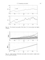
Fig. 14.2. Implied volatility against exercise price for some FTSE 100 index
data.
The initial asset price (on 22 August 2001) was 5420.3. We took values of r =
0.05 for the interest rate and T = 4/12 for the duration of the option. Figure 14.2
shows the implied volatility computed for the eight different exercise prices. Of
course, if the Black–Scholes formula were valid, the volatility would be the same
for each exercise price. We see that in this example the implied volatility varies
by around 10%. We also note that the implied volatility is higher for options that
start in-the-money than for options starting out-of-the-money. This behaviour is
14.7 Program of Chapter 14 and walkthrough 137
typical for data arising after the stock market crash of October 1987. Pre-crash
plots of implied volatility against exercise price would often produce a convex
smile shape; more recent data tends to produce more of a frown.
14.6 Notes and references
The convergence analysis for Newton’s method is based on the article (Manaster
and Koehler, 1982). It is also mentioned in (Kwok, 1998). More about implied
volatility can be found in (Hull, 2000; Kwok, 1998), for example.
The widely reported phenomenon that the implied volatility is not constant as
other parameters are varied does, of course, imply that the Black–Scholes formu-
las fail to describe perfectly the option values that arise in the marketplace. This
should be no surprise, given that the theory is based on a number of simplifying as-
sumptions. Despite the disparities, the Black–Scholes theory, and the insights that
it provides, continue to be regarded highly by both academics and market traders.
Indeed, it is common for option values to be quoted in terms of ‘vol’; rather than
giving C

, the σ

such that C(σ


) = C

in the Black–Scholes formula is used to
describe the value.
Many attempts have been made to ‘fix’ the nonconstant volatility discrepancy
in the Black–Scholes theory. A few of these have met with some success, but
none lead to the simple formulas and clean interpretations of the original work.
Chapter 17 of (Hull, 2000) gives a good overview of the directions that have been
taken.
EXERCISES
14.1.  Show that ∂C/∂σ has a unique maximum over [0, ∞) at σ = σ,
where σ is defined in (14.5).
14.2.  Verify the identity (14.6).
14.3. Suppose σ
0
= σ. Using the fact that F

(σ ) > 0 for σ<σ , confirm
that (14.10) holds in the case where σ>σ

.
14.7 Program of Chapter 14 and walkthrough
In ch14, listed in Figure 14.3, we implement Newton’s method for implied volatility of a European
call. After setting up r,S,E,T and tau,weusech08 from Chapter 8 to compute the call value,
C_true, corresponding to a volatility of sigma_true=0.3. Our task is then to recover the volatility
that produces the call value C_true.Weuse a while loop of the form discussed for ch13,witha
call to ch10 providing the required vega value. The final solution is correct to within 6 × 10
−17
.

138 Implied volatility
%CH14 Program for Chapter 14
%
% Computes implied volatility for a European call
%%%%%%%%%%% parameters %%%%%%%%%%
r=0.03;S=2;E=2;T=3;tau=T;sigma
true = 0.3;
[C
true, Cdelta, P, Pdelta] = ch08(S,E,r,sigma true,tau);
%%%%%%%%%%%%%%%%%%%%%%%%%%%%
%starting value
sigmahat = sqrt(2*abs( (log(S/E) + r*T)/T ) );
%%%%%% Newton’s method %%%%%
tol = 1e-8;
sigma = sigmahat;
sigmadiff = 1;
k=1;
kmax = 100;
while (sigmadiff >= tol&k<kmax)
[C, Cdelta, Cvega, P, Pdelta, Pvega] = ch10(S,E,r,sigma,tau);
increment = (C-C
true)/Cvega;
sigma = sigma - increment;
k=k+1;
sigmadiff = abs(increment);
end
sigma
Fig. 14.3. Program of Chapter 14: ch14.m.
PROGRAMMING EXERCISES
P14.1. Alter ch14 to deal with a put option.

P14.2. Acquire some real option data, either electronically or via a newspaper,
and create a figure like Figure 14.2. If possible, investigate the behaviour of the
implied volatility as the expiry time varies.
Quotes
The volatility is the most important and elusive quantity
in the theory of derivatives.
PAUL WILMOTT (Wilmott, 1998)
A smiley implied volatility is the wrong number
to put in the wrong formula
to obtain the right price.
RICCARDO REBONATO (Rebonato, 1999)
It is the strong opinion of the author that most traders
14.7 Program of Chapter 14 and walkthrough 139
will gain an improved performance by concentrating their efforts
on a better prediction of the volatility input into a Black–Scholes type model
rather than introducing other pricing techniques.
A . L . H. SMITH (Smith, 1986)
In those days, before the publication of the Black–Scholes option-pricing formula,
warrants were often grossly mispriced. Thorpe soon developed a computer program
to identify such opportunities; its deployment was so successful that,
by 1970, both Thorpe and Kassouf had abandoned academe for greener pastures.
JAMES CASE,reviewing the book (Bass, 1999) in Society for Industrial and Applied
Mathematics (SIAM) News, Jan/Feb, 2001.

15
Monte Carlo method
OUTLINE
• Monte Carlo
• confidence intervals
• Monte Carlo for option valuation

• Monte Carlo for Greeks
15.1 Motivation
Chapter 12 showed that valuing an option can be regarded as computing an ex-
pected value. The idea of using pseudo-random number generators to compute
estimates of expected values was touched on in Chapter 4. Here we pull these two
threads together and introduce the Monte Carlo approach to valuing an option.
As we will see in Chapter 19, this provides a powerful means to compute option
values in cases where no analytical formulas are available.
15.2 Monte Carlo
To begin, we consider the case of a general random variable X, whose expected
value
E(X ) = a and variance var(X) = b
2
are not known. Suppose
• we are interested in computing an approximation to a (and possibly b), and
• we are able to take independent samples of X using a pseudo-random number generator.
We know from Table 4.2 that computing the average of a large number of samples
can give a good approximation to the mean. Hence, if we let X
1
, X
2
, ,X
M
denote independent random variables with the same distribution as X then we
might expect
a
M
:=
1
M

M

i=1
X
i
(15.1)
141
142 Monte Carlo method
to be a good approximation to a.Wesay that an approximation to E(X) is un-
biased if it has the same expected value as X.Itiseasily shown that a
M
in
(15.1) is unbiased; see Exercise 15.1. To estimate the variance, since var(X) :=
E((X − E(X))
2
),anobvious choice is (

M
i=1
(X
i
− a
M
)
2
)/M.However, to make
this estimate unbiased we need to re-scale it slightly. Exercise 15.2 asks you to
check that the appropriate unbiased version is
b
2

M
:=
1
M − 1
M

i=1
(X
i
− a
M
)
2
. (15.2)
By the Central Limit Theorem,

M
i=1
X
i
behaves like an N(Ma, Mb
2
) random
variable, so
a
M
− a is approximately N

0,
b

2
M

. (15.3)
We could also say that a
M
− a is approximately an N(0, 1) random variable scaled
by b/
√
M. This suggests that sampling a
M
for large M should give an approxima-
tion to a that is correct to O(1/
√
M).
We can make this argument more quantitative by using the idea of a confidence
interval that was introduced in Section 6.5. If we had equality in (15.3) then, from
(6.15),
P

a −
1.96 b
√
M
≤ a
M
≤ a +
1.96 b
√
M


= 0.95.
We may re-write this as
P

a
M
−
1.96 b
√
M
≤ a ≤ a
M
+
1.96 b
√
M

= 0.95. (15.4)
The ratio b/
√
M appearing in (15.4) is often refered to as the standard error. Re-
placing the unknown b by the approximation b
M
we see that the unknown expected
value a lies in the interval

a
M
−

1.96 b
M
√
M
, a
M
+
1.96 b
M
√
M

(15.5)
with probability 0.95, approximately. In other words (15.5) gives an approximate
95% confidence interval for a.
This analysis leads us to the basic Monte Carlo method for approximating a.We
compute M independent samples and form a
M
in (15.1). In order to monitor the
error, we also compute the variance approximation b
2
M
in (15.2). Having b
M
allows
us to compute the confidence interval (15.5) (or indeed, a confidence interval for
some other percentage, such as 99%; see Exercise 6.8).
15.2 Monte Carlo 143
10
1

10
2
10
3
10
4
10
5
10
6
10
0.1
10
0.2
10
0.3
10
0.4
Num samples
Sample mean
Fig. 15.1. Monte Carlo approximations to E(e
Z
), where Z ∼ N(0, 1).Crosses
are the approximations, vertical lines give computed 95% confidence intervals.
Horizontal dashed line is at height E(e
Z
) =
√
e.
There are two key features to note.

(i) The size of the confidence interval shrinks like the inverse square root of the number
of samples. To reduce the ‘error’ by a factor of 10 requires a hundredfold increase in
the sample size. This is a severe limitation that typically makes it impossible to get
very high accuracy from a Monte Carlo approximation.
(ii) The size of the confidence interval is directly proportional to the standard deviation,
that is the square root of the variance, of the random variable under consideration. In
practice, it is highly desirable to transform the problem of approximating E(X) to the
problem of approximating E(Y ) where Y is another random variable that has the same
mean as X butasmaller variance. This idea, known as variance reduction, forms a
vital part of practical Monte Carlo algorithms. The two most popular approaches are
covered in Chapters 21 and 22.
Computational example In Figure 15.1 we give results from a Monte Carlo
simulation of
E(e
Z
), where Z ∼ N(0, 1).Inthis case we can work out analyt-
ically that
E(e
Z
) =
√
e; see Exercise 15.3. We used 13 different sample sizes,
M = 2
5
, 2
6
, 2
7
, ,2
17

.For each sample size, the picture plots the computed
mean, a
M
, with a cross and gives the computed 95% confidence interval as a
vertical line, often called an error bar. Note that both axes have logarithmic
scales. The exact mean,
√
e,isrepresented as a dashed line. We see that as M in-
creases the computed mean generally becomes more accurate and the confidence
144 Monte Carlo method
interval shrinks. In the third case, M = 2
7
, the correct mean is not contained in
the confidence interval. Remember that our theory predicts that this will happen
roughly 5% of the time, but requires M sufficiently large that
• the Central Limit Theorem approximation is accurate, and
• the computed variance b
M
approximates well the exact variance b.
A separate check revealed that with M = 2
7
the variance error |b
2
M
− b
2
| was a
non-negligible 7.1. The errors for M = 2
16
and M = 2

17
are 5.31 × 10
−3
and
3.64 × 10
−3
, respectively. The ratio of these errors is ≈ 1.5, which is close to
the asymptotic (M →∞)value of
√
2. This computation is typical – we have
achieved a few digits of accuracy with a modest amount of work. The ‘curse of
the 1/
√
M’ makes higher accuracy extremely costly. To reduce the error to, say,
10
−4
would take of the order of 10
8
samples, and to reduce it to 10
−6
would take
of the order of 10
12
samples; see Exercise 15.4. ♦
15.3 Monte Carlo for option valuation
We are now in a position to use Monte Carlo for option valuation. We consider
a European-style option with payoff that is some function  of the asset price at
expiry. Our model for the asset price at expiry is (6.8) with t = T . Using the risk
neutrality approach discussed in Chapter 12, the time-zero option value can be
found by setting µ = r and computing e

−rT
E((S(T ))).
Putting all this together, we wish to find the expected value of the random vari-
able
e
−rT


S
0
exp

r −
1
2
σ
2

T + σ
√
TZ

, where Z ∼ N(0, 1). (15.6)
The resulting Monte Carlo algorithm can be summarized as follows:
for i =1toM
compute an N(0, 1) sample ξ
i
set S
i
= S

0
e
(r−
1
2
σ
2
)T +σ
√
T ξ
i
set V
i
= e
−rT
(S
i
)
end
set a
M
=

1
M


M
i=1
V

i
set b
2
M
=

1
(M−1)


M
i=1
(V
i
− a
M
)
2
The output provides an approximate option price a
M
and an approximate 95%
confidence interval (15.5).
Computational example We now use the Monte Carlo method to value a
European call option, so (S(T )) = max(S(T ) − E, 0).Wewill use the
Black–Scholes formula (8.19) to compute the exact value and then see how
15.4 Monte Carlo for Greeks 145
10
1
10
2

10
3
10
4
10
5
10
6
10
0.1
10
0.2
10
0.3
Num samples
Option value approximation
Fig. 15.2. Monte Carlo approximations to a European call option value. Crosses
are the approximations, vertical lines give computed 95% confidence intervals.
Horizontal dashed line is at height given by the Black–Scholes formula.
well Monte Carlo performs. We take S
0
= 10, E = 9, σ = 0.1, r = 0.06 and
T = 1. The Black–Scholes option value is 1.5429. Figure 15.2 shows the Monte
Carlo results, in a similar manner to Figure 15.1. We used sample sizes M =
2
5
, 2
6
, ,2
17

.For each sample size we plot the computed mean a
M
with a
cross and show the computed 95% confidence interval as a vertical line. The
same pseudo-random number sequences as those for Figure 15.1 were used, and
once again the M = 2
7
confidence interval does not contain the true mean. With
the largest sample size, 2
17
, the error in a
M
was ≈ 1.2 × 10
−3
.Weemphasize
that in this example there is no need to apply Monte Carlo as the Black–Scholes
formula gives the exact solution conveniently. However, as we will see in Chap-
ter 19, Monte Carlo comes into its own in more complicated circumstances where
no simple Black–Scholes-type formula is available. ♦
15.4 Monte Carlo for Greeks
In addition to the option value, we know that the Greeks – the partial derivatives
of the option value with respect to various quantities – are also of interest. In
particular, the delta,  := ∂V /∂ S,plays a key role in the hedging strategy that a
trader must operate in order to replicate the option. The Monte Carlo approach can
be used to compute approximate partial derivatives; although it must be handled
146 Monte Carlo method
with care and may prove expensive. We focus here on the case of computing the
time-zero delta of a European-style option with payoff (S(T )),but the principles
apply generally.
A simple Taylor series expansion shows that the delta at asset price S and time

t satisfies
∂V (S, t)
∂ S
=
V (S + h, t) − V (S, t)
h
+ O(h), as h → 0. (15.7)
Hence, we may choose a small value of h and use the finite difference approxima-
tion
∂V (S, t)
∂ S
≈
V (S + h, t) − V (S, t)
h
.
This produces an approximation to delta at a single point based on option values at
two points with slightly different S arguments. Using the risk-neutral, discounted,
expected payoff formulation, we could thus approximate the time-zero delta by
computing Monte Carlo estimates of the two expected values in
e
−rT
E
(
(S(T )), with S(0) = S
0
)
−
E
(
(S(T )), with S(0) = S

0
+ h
)
h
.
(15.8)
Now the error in each of the two Monte Carlo estimates is O(1/
√
M) and hence,
after dividing the difference by h,weexpect an overall error of O(1/(h
√
M))
for (15.8). This is unfortunate: we want to make h small to get a good derivative
approximation in (15.7), but doing so forces us to take even more samples than
the basic Monte Carlo option value strategy would need. Another way to view the
difficulty is to note that in order to satisfy ourselves that we have even got the
correct sign for the delta, we might ask for non-overlapping confidence intervals
from the two Monte Carlo approximations. Since the exact means V (S, t) and
V (S + h, t) differ by O(h), this requires confidence interval widths that are at
least as small as O(h).
However, we can claw back some accuracy by noting that the two random vari-
ables in (15.8) are highly correlated: for any particular asset path the payoff start-
ing from S(0) = S
0
is likely to be close to the payoff starting from S
0
+ h. In-
tuitively, the corresponding sample mean errors should be close provided that we
use the same paths for the two simulations; that is we apply Monte Carlo to the
equivalent problem

e
−rT
E
[
(
(S(T )), with S(0) = S
0
)
−
(
(S(T )), with S(0) = S
0
+ h
)
]
h
,
(15.9)
15.4 Monte Carlo for Greeks 147
which involves a single random variable. In Chapters 21 and 22 we make the idea
of correlation more explicit, and Exercise 22.3 gives further justification for this
argument.
This leads us to the following Monte Carlo algorithm for approximating .
for i =1toM
compute an N(0, 1) sample ξ
i
set S
i
= S
0

e
(r−
1
2
σ
2
)T +σ
√
T ξ
i
set S
h
i
= (S
0
+ h)e
(r−
1
2
σ
2
)T +σ
√
T ξ
i
set 
i
= e
−rT
((S

i
) −(S
h
i
))/ h
end
set a
M
=
1
M

M
i=1

i
set b
2
M
=
1
M−1

M
i=1
(
i
− a
M
)

2
This produces an approximate delta value a
M
and an approximate 95% confidence
interval (15.5).
Computational example Here we return to the European call option used for
Figure 15.2 with the same sample sizes M. The Black–Scholes time-zero delta
value is 0.9558. Figure 15.3 shows the corresponding delta approximations from
10
1
10
2
10
3
10
4
10
5
10
6
10
−0.08
10
−0.06
10
−0.04
10
−0.02
10
0

10
0.02
Num samples
Delta approximation
Fig. 15.3. Monte Carlo approximations to time-zero delta of a European call
option. Crosses are the approximations, vertical lines give computed 95% confi-
dence intervals. Horizontal dashed line is at height given by the Black–Scholes
formula.
148 Monte Carlo method
the algorithm above, in the style of Figures 15.1 and 15.2. We fixed h = 10
−4
.
For M = 2
17
, the error in the sample was ≈ 1.2 × 10
−4
; smaller than that for the
corresponding Monte Carlo option value approximation. We also experimented
with the corresponding algorithm that uses different pseudo-random numbers for
the two options. The results were much worse; for the M values used here, no
digits of accuracy were recorded, and the standard deviations were around 50 000
times larger. ♦
15.5 Notes and references
There are many texts that discuss general Monte Carlo simulation. A ‘golden oldie’
that is still highly relevant is (Hammersley and Handscombe, 1964), whilst a short
and very accessible modern perspective is given by (Madras, 2002). Monte Carlo,
pseudo-random number generation and other simulation issues are treated in detail
in (Ripley, 1987).
Boyle’s classic 1977 paper (Boyle, 1977), which won the Journal of Financial
Economics’ All-Star Paper Award 2002, introduced Monte Carlo for option val-

uation. The paper (Boyle et al., 1997) summarizes developments since then, and
in particular, has a detailed treatment of the Greeks. Texts that cover Monte Carlo
for finance in some depth include (Clewlow and Strickland, 1998; J
¨
ackel, 2002;
Kwork, 1998)
EXERCISES
15.1.  Show that a
M
in (15.1) is an unbiased estimator of E(X ); that is, E(a
M
) =
a.
15.2. Show that

b
2
M
:=
1
M
M

i=1
(X
i
− a
M
)
2

satisfies
E(

b
2
M
) =

M − 1
M

b
2
. (15.10)
This confirms that

b
M
2
is not an unbiased estimator of var(X). Conclude
from (15.10) that b
M
2
in (15.2) is an unbiased estimator of var(X ).
15.3.  Show that if Z ∼ N(0, 1) then
E(e
Z
) =
√
e.[Hint: recall (3.8).]

15.4.  For the computational experiment that produced Figure 15.1, it was pre-
dicted that ‘To reduce the error to, say, 10
−4
,would take of the order of 10
8
15.6 Program of Chapter 15 and walkthrough 149
%CH15 Program for Chapter 15
%
% Monte Carlo for a European put
randn(’state’,100)
%%%%%%%%%%% Problem and method parameters %%%%%%%%%
S=4;E=5;sigma = 0.3;r=0.04;T=1;
Dt = 1e-3;N=T/Dt;M=1e4;
%%%%%%%%%%%%%%%%%%%%%%%%%%%%%%%%%%%%%%
V=zeros(M,1);
for i = 1:M
Sfinal = S*exp((r-0.5*sigmaˆ2)*T+sigma*sqrt(T)*randn);
V(i) = exp(-r*T)*max(E-Sfinal,0);
end
aM = mean(V); bM = std(V);
conf = [aM - 1.96*bM/sqrt(M), aM + 1.96*bM/sqrt(M)]
Fig. 15.4. Program of Chapter 15: ch15.m.
samples, and to reduce it to 10
−6
would take of the order of 10
12
samples.’
Where do these figures come from? For the computations in Figure 15.2,
roughly how many samples would be needed to reduce the error to 10
−6

?
15.6 Program of Chapter 15 and walkthrough
In ch15, listed in Figure 15.4, we use Monte Carlo to value a European put. The code follows
the algorithm in Section 15.3, making use of MATLAB’s built-in functions mean and std, which,
respectively, compute the sample mean (15.1) and sample standard deviation – the square root of the
sample variance (15.2).
The code produces a confidence interval conf = [1.0070, 1.0402]. Checking with the
Black–Scholes formula from ch08 gives
>> [C, Cdelta, P, Pdelta] = ch08(4,5,0.04,0.3,1)
C=0.2167
Cdelta = 0.3226
P=1.0207
Pdelta = -0.6774
PROGRAMMING EXERCISES
P15.1. Adapt ch15 to produce a picture like that in Figure 15.2.
P15.2. Adapt
ch15 to produce an estimate of the delta.
150 Monte Carlo method
Quotes
To know the vintage and quality of a wine
one need not drink the whole cask.
OSCAR WILDE, 1854–1900.
In the classical theory, which we are discussing here,
the unknown parameter p is a number, not a random variable,
so p is either in I or outside it,
and it is meaningless to speak of the probability of p lying in I
(the Bayesians, on the other hand, consider p a random variable – see Section 15.7).
The expression 95% confidence interval refers to the
procedure through which I was produced.
This procedure produces intervals containing p 95 percent of the time.

RICHARD ISAAC (Isaac, 1995)
The Central Limit Theorem is a powerful tool,
and we wish we had an intuitive explanation of why it should be true.
Unfortunately, we don’t.
MARK DENNEY AND STEVEN GAINES (Denney and Gaines, 2000)
16
Binomial method
OUTLINE
• description of the binomial method
• derivation of the parameters
• computational results
16.1 Motivation
We now introduce another computational approach. The binomial method is
straightforward to describe and implement, and, as we will see in Chapters 18
and 19, has the advantage that it is readily adapted to a range of non-European
options for which no analytical formula is available. In particular, the bino-
mial method provides the simplest means to value American options. In study-
ing the method, we revisit two ideas, discrete asset price models and risk
neutrality.
16.2 Method
The binomial method uses a simple discrete model for the asset price movement.
We let δt = T/M denote the spacing between successive time points, where T
is the expiry date. So asset prices will be considered at times t
i
= iδt, for 0 ≤
i ≤ M.Akey assumption in the binomial method is that between successive time
levels the asset price moves either up by a factor u or down by a factor d.An
upward movement occurs with probability p and a downward movement occurs
with probability 1 − p. This scenario can be regarded as a simplified version of
the discrete model introduced in Chapter 6. Indeed, Exercise 16.1 asks you to cast

this simple model in the form (6.2) by redefining Y
i
.
Since the initial asset price, S
0
,isknown, at time t
1
= δt the possible asset
prices are uS
0
and dS
0
. Similarly, at time t
2
= 2δt the possible asset prices are
151
152 Binomial method
S
0
S
1
1
S
1
0
S
2
2
S
2

1
S
2
0
S
M
M
S
M
M
1
S
M
0
S
M
1
Fig. 16.1. Recombining binary tree of asset prices.
u
2
S
0
, udS
0
and d
2
S
0
. (The price udS
0

may arise from an upward movement
followed by a downward movement or from a downward movement followed by
an upward movement.) In general, at time t = t
i
:= iδt there are i + 1 possible
asset prices, which we label
S
i
n
= d
i−n
u
n
S
0
, 0 ≤ n ≤ i. (16.1)
Hence, at the expiry time t = t
M
= T there are M + 1 possible asset prices. The
values S
i
n
for 0 ≤ n ≤ i and 0 ≤ i ≤ M form a recombining binary tree, as illus-
trated in Figure 16.1.
ForaEuropean-style call option, the payoff at expiry has the form (S(T)).
Hence, if the asset has price S
M
n
at time t = t
M

= T then the value of the option
at that time is (S
M
n
). Generally, we let V
i
n
denote the value of the option at time
t = t
i
corresponding to asset price S
i
n
.Wethus know that
V
M
n
= (S
M
n
), 0 ≤ n ≤ M. (16.2)