An Introduction to Financial Option Valuation: Mathematics, Stochastics and Computation_9 pot

16.3 Deriving the parameters 153
Our task is to find V
0
0
, the option value at time zero. We may do this by working
backwards through the tree. Suppose {V
i+1
n
}
i+1
n=0
are known; that is, we have the
option values corresponding to time t = t
i+1
and all possible asset prices. Then
consider the option value V
i
n
corresponding to asset price S
i
n
at time t = t
i
.Because
of our up/down assumption about the asset price movement, working from right to
left, the asset price S
i
n
comes either from S
i+1
n+1

, with probability p,orfrom S
i+1
n
,
with probability 1 − p.Now, recall the definition (3.1) for the expected value of
a discrete random variable. The big idea in the binomial method is to multiply
the two possible values V
i+1
n+1
and V
i+1
n
by their associated probabilities to get an
expected value. In this way the option value V
i
n
corresponding to asset price S
i
n
is
taken to be pV
i+1
n+1
+ (1 − p)V
i+1
n
,scaled by the appropriate factor that allows for
the interest rate, r. This gives the fundamental relation
V
i

n
= e
−rδt

pV
i+1
n+1
+ (1 − p)V
i+1
n

, 0 ≤ n ≤ i, 0 ≤ i ≤ M − 1.
(16.3)
Once the parameters u, d, p and M have been chosen, the formulas (16.1)–
(16.3) completely specify the binomial method. The recurrence (16.1) shows how
to insert the asset prices in the binomial tree. Having obtained the asset prices at
time t = t
M
= T , (16.2) gives the corresponding option values at that time. The
relation (16.3) may then be used to step backwards through the tree until V
0
0
, the
option value at time t = t
0
= 0, is computed.
16.3 Deriving the parameters
Since the discrete asset price model in the binomial method fits into the framework
of (6.2), by appealing to Exercise 6.2 we could tune the parameters by asking for
the corresponding Y

i
to have zero mean and unit variance. This would lead to
two constraints. However, to give more insight into the workings of the method,
we will derive those constraints from first principles. Exercise 16.5 asks you to
confirm that the two approaches lead to the same conclusion.
As a means to write down an expression for the up/down asset price model used
in the binomial method, we define a random variable R
i
such that R
i
= 1ifthe
asset price goes up from time (i − 1)δt to iδt and R
i
= 0ifthe asset price goes
down. Hence, R
i
= 1 with probability p and R
i
= 0 with probability 1 − p. This
means that R
i
is a Bernoulli random variable with parameter p,sofrom (3.2) and
(3.14) we see that
E(R
i
) = p and var(R
i
) = p(1 − p). After n time increments
the asset has undergone


n
i=1
R
i
upward movements and n −

n
i=1
R
i
downward
movements. So the asset price S(nδt) at time t = nδt is given by
S(nδt) = S
0
u

n
i=1
R
i
d
n−

n
i=1
R
i
.
154 Binomial method
We may re-arrange this to

S(nδt)
S
0
= d
n

u
d


n
i=1
R
i
.
Taking logs gives
log

S(nδt)
S
0

= n log d + log

u
d

n

i=1

R
i
. (16.4)
Now, by the Central Limit Theorem, for large n the sum

n
i=1
R
i
behaves like
a normal random variable. Hence, for large n, log(S(nδt)/S
0
) will be close to
normal. To match the continuous asset price model (6.8) used in the Black–Scholes
analysis, we thus require the mean of log(S(nδt)/S
0
) to be (µ −
1
2
σ
2
)nδt and the
variance to be σ
2
nδt. Further, as the binomial method works with expected values,
we impose the risk neutrality assumption µ = r. This leads to the conditions
p log u + (1 − p) log d = (r −
1
2
σ

2
)δt, (16.5)
log

u
d

= σ

δt
p(1 − p)
, (16.6)
see Exercise 16.2. Regarding δt = T/M as pre-specified, we now have two equa-
tions in the three unknowns, p, u and d.Ingeneral, we can fix one of the three
and solve for the other two. To pick out a particular solution this way, we may set
p =
1
2
and solve to find that
u = e
σ
√
δt+(r−
1
2
σ
2
)δt
, d = e
−σ

√
δt+(r−
1
2
σ
2
)δt
, (16.7)
see Exercise 16.3.
16.4 Binomial method in practice
The arguments in the previous section suggest that the binomial method asset
model matches that used in the Black–Scholes analysis for small δt, that is, large
M.Wemay thus hope that the option values computed from the binomial method
agree well with those from the Black–Scholes formulas, and that the agreement
improves if M is increased.
Computational example We use the binomial method to value a European
put with S
0
= 9, E = 10, T = 3, r = 0.06 and σ = 0.3. Table 16.1 shows the
results for M = 100, M = 200 and M = 400, along with the Black–Scholes
value 1.4728. Our first observation is that with all three choices of M the bi-
nomial method approximation is correct to at least two decimal places. The
16.4 Binomial method in practice 155
Table 16.1. European put value
approximations from binomial method
Option value
M = 100 1.4716
M = 200 1.4762
M = 400 1.4726
Black–Scholes 1.4728

0 50 100 150 200 250
1.46
1.48
1.5
1.52
M
European put
200 220 240 260 280 300 320 340 360 380 400
1.472
1.473
1.474
1.475
1.476
1.477
M
European put
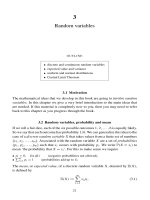
Fig. 16.2. Convergence of the binomial method for a European put as the num-
ber of time points, M, increases. Upper picture: M goes from 20 to 250 in steps
of 5. Dashed line is ‘exact’ solution. Lower picture: M goes from 200 to 400 in
steps of 1.
most accurate approximation of the three comes from the largest value of M,
which is intuitively reasonable. However, it is perhaps surprising that M = 200
gives less accuracy that M = 100. To check whether this is simply a quirk,
the upper picture in Figure 16.2 shows the computed option value for M =
20, 25, 30, ,250, with the Black–Scholes value superimposed as a dashed
line. We see that although the binomial method approximations do appear to
converge as M increases, the convergence is by no means monotonic – tak-
ing a slightly bigger M may worsen the error – and there is a general ‘saw-
tooth’ pattern to the sequence of approximations as M increases. The lower plot
156 Binomial method

emphasizes the waviness. Here we have plotted the computed solution for all M
between 200 and 400. The result appears to oscillate between two smooth curves,
neither of which approaches the correct answer monotonically. ♦
Two features stand out in Figure 16.2.
(i) The binomial method approximation converges to the Black–Scholes value as
M →∞.
(ii) The convergence is not monotonic.
These may be shown to be generic. Moreover, it is possible to describe the rate at
which convergence takes place. Letting e
M
=|V
0
0
− P(S
0
, 0)| denote the error in
the binomial method approximation with δt = T/M,itcan be shown that there is
a constant K such that
e
M
≤
K
M
. (16.8)
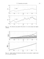
In the upper picture of Figure 16.3 we display the errors in the example above for
M between 100 and 400. The points have been joined by straight lines for clarity.
The curve 1/M is added as a solid line, and we see that (16.8) appears to hold with
K = 1. Taking logs in (16.8) gives log e
M
≤ log K − log M,showing that the log

of the error as a function of log M should lie below a straight line of slope −1.
The lower picture of Figure 16.3 re-scales the axes logarithmically to confirm this
behaviour.
16.5 Notes and references
Cox, Ross and Rubinstein (Cox et al., 1979) wrote the original binomial method
paper. Since then numerous authors have analysed and extended the ideas.
It is possible to derive the parameters u, d and p from a number of different
viewpoints. For example, with p =
1
2
the choice
u = e
rδt

1 +

e
σ
2
δt
− 1

, d = e
rδt

1 −

e
σ
2

δt
− 1

(16.9)
is common; see (Kwok, 1998; Wilmott et al., 1995). Exercise 16.4 shows that this
is very close to the choice (16.7) for small δt.
Although much literature has been devoted to establishing that the error in vari-
ous classes of binomial methods tends to zero as M →∞, surprisingly little atten-
tion was initially paid to the rate of convergence. Leisen and Reimer (Leisen and
Reimer, 1996) developed a general convergence rate theory, and the bound (16.8)
follows from their results. A more detailed analysis, with explicit error constants,
appears in (Walsh, 2003).
16.5 Notes and references 157
100 150 200 250 300 350 400
0
0.002
0.004
0.006
0.008
0.01
M
Error in binomial method
100 200 400
10
−6
10
−4
10
−2
M

Error in binomial method
Fig. 16.3. Upper picture: Error in the binomial method for a European put as the
number of time points, M, increases from 100 to 400. Solid line is 1/M.Lower
picture: same data on a log–log scale.
The odd–even ripples in the error, as depicted in Figures 16.2 and 16.3, have
been widely reported. The references (Leisen and Reimer, 1996; Rogers and Sta-
pleton, 1998) give explanations for the effect and propose fixes.
Applying the binomial method may be shown to be equivalent to using a finite
difference method to approximate the Black–Scholes PDE, a point that we pursue
in Section 24.4. This is one means of proving that the binomial method solution
converges to the Black–Scholes value as M →∞, see (Kwok, 1998), for example,
and numerical analysis insights can also be used to explain the odd-even ripples.
The book (Clewlow and Strickland, 1998) covers a number of practical issues
in the implementation of the binomial method, and provides pseudo-code listings.
A case study with the aim of making the binomial method run as quickly as
possible in MATLAB is given in (Higham, 2002), along with downloadable codes.
It is possible to compute Greeks via the binomial method. For partial derivatives
with respect to S or t, approximations can be obtained using information from the
tree. Exercise 16.8 illustrates the idea. Other partial derivatives can be treated by
re-running the method with perturbed data, in the manner outlined in Section 15.4.
Further details can be found in (Hull, 2000), for example, and (Walsh, 2003) shows
that delta can be approximated to the same order of accuracy as the option value.
158 Binomial method
EXERCISES
16.1.  Consider the discrete asset price model used in the binomial method.
Show that it may be written in the form (6.2) if we let Y
i
be defined as
Y
i

=



u−1−µδt
σ
√
δt
, with probability p,
d−1−µδt
σ
√
δt
, with probability 1 − p.
(16.10)
16.2.  Starting from (16.4) show that
E

log

S(nδt)
S
0

= n log d + log

u
d

np

and
var

log

S(nδt)
S
0

=

log

u
d

2
np(1 − p).
Hence, obtain (16.5)–(16.6).
16.3.  Show that setting p =
1
2
in (16.5)–(16.6) produces (16.7).
16.4. For the parameters u and d in (16.7) show that
u = 1 + σ
√
δt + rδt + O(δt
3/2
), d = 1 − σ
√

δt + rδt + O(δt
3/2
),
as δt → 0.
Show also that the corresponding u and d parameters in (16.9) have the
same expansions up to O(δt
3/2
). [Hint: recall that
√
1 + x = 1 +
1
2
x +
O(x
2
) and e
x
= 1 + x +
1
2
x
2
+ O(x
3
) as x → 0.]
16.5.  We know from Exercise 6.2 that if Y
i
in (16.10) has zero mean and unit
variance, we recover the continuous asset price model in the limit δt → 0.
Set µ = r and p =

1
2
and show that requiring E(Y
i
) = 0 and var(Y
i
) = 1
in (16.10) leads to
u = 1 + σ
√
δt + rδt, d = 1 − σ
√
δt + rδt.
Note that these values agree with those in Exercise 16.4 up to O(δt
3/2
).
16.6. Returning to the recurrence (16.3) we see that for M = 1
V
0
0
= e
−rδt

pV
1
1
+ (1 − p)V
1
0


,
and for M = 2
V
0
0
= e
−rδt

pV
1
1
+ (1 − p)V
1
0

= e
−rδt

pe
−rδt
( pV
2
2
+ (1 − p)V
2
1
) + (1 − p)e
−rδt
( pV
2

1
+(1 − p)V
2
0
)

= e
−2rδt

p
2
V
2
2
+ 2p(1 − p)V
2
1
+ (1 − p)
2
V
2
0

.
16.6 Program of Chapter 16 and walkthrough 159
Similarly for M = 3wefind that
V
0
0
= e

−3rδt

p
3
V
3
3
+ 3p
2
(1 − p)V
3
2
+ 3p(1 − p)
2
V
3
1
+ (1 − p)
3
V
3
0

.
The coefficients {1, 1}, {1, 2, 1}, {1, 3, 3, 1} are familiar from Pascal’s tri-
angle. Having spotted this connection, prove by induction that
V
0
0
= e

−rT
M

k=0

M
k

p
k
(1 − p)
M−k
V
M
k
, (16.11)
where

M
k

denotes the binomial coefficient,

M
k

:=
M!
k! (M − k)!
.

16.7.  Letting
W
i
:=








V
i
0
V
i
1
.
.
.
.
.
.
V
i
i









,
write down the form of the i by (i + 1) matrix B
i
such that W
i
= B
i
W
i+1
.
16.8.  Explain why the ratio (V
1
1
− V
1
0
)/(S
1
1
− S
1
0
) can be regarded as an ap-
proximation to the time-zero delta.
16.6 Program of Chapter 16 and walkthrough

The program ch16 implements the binomial method for a European call. It is listed in Figure 16.4.
First, parameters are initialized, using (16.7) for u and d. The quantity
S*d.^([M:-1:0]’).*u.^([0:M]’)
is an M+1 by 1 array whose components cover the values S
M
0
, S
M
1
, ,S
M
M
in the expiry-time level
of the asset price tree in Figure 16.1. Hence, the line
W=max(S*d.^([M:-1:0]’).*u.^([0:M]’)-E,0);
contains the expiry time option values, as in (16.2). We then work through the iteration (16.3) by
exploiting MATLAB’s colon notation to extract subarrays. The syntax
exp(-r*dt)*(p*W(2:i+1) + (1-p)*W(1:i));
160 Binomial method
%CH16 Program for Chapter 16
%
% Implements binomial method for European call
%%%%%%%% Problem and method parameters %%%%%%%%%%%
S=3;E=2;T=1;r=0.05; sigma = 0.3;
M=400; dt = T/M; p =0.5;
u=exp(sigma*sqrt(dt) + (r-0.5*sigmaˆ2)*dt);
d=exp(-sigma*sqrt(dt) + (r-0.5*sigmaˆ2)*dt);
%%%%%%%%%%%%%%%%%%%%%%%%%%%%%%%%%%%%%
%Time T option values
W=max(S*d.ˆ([M:-1:0]’).*u.ˆ([0:M]’)-E,0);

%Work back to option value at time zero
for i = M:-1:1
W=exp(-r*dt)*(p*W(2:i+1) + (1-p)*W(1:i));
end
disp(’Option value is’), disp(W)
Fig. 16.4. Program of Chapter 16: ch16.m.
represents
e
−rδt






p






W
2
W
3
.
.
.
W

i+1






+ (1 − p)






W
1
W
2
.
.
.
W
i













.
The line for i = M:-1:1 sets up a loop that is repeated M times; first with i=M, then with i=
M-1,andso on, down to i=1.With this set-up, the dimension of W decreases by one each time
around the loop. On exit, W is a scalar, whose value is V
0
0
.
Running ch16.m produces the value 1.1175.Tocheck, we may call ch08.
>> [C, Cdelta, P, Pdelta] = ch08(3,2,0.05,0.3,1)
C=1.1175
Cdelta = 0.9524
P=0.0200
Pdelta = -0.0476
PROGRAMMING EXERCISES
P16.1. Alter ch16 so that the choice (16.9) for u and d is used.
P16.2. Implement the binomial method via the formula (16.11).
16.6 Program of Chapter 16 and walkthrough 161
Quotes
‘Would you tell me, please, which way I ought to go from here?’
‘That depends a good deal on where you want to get to,’ said the Cat.
‘I don’t much care where ’said Alice.
‘Then it doesn’t matter which way you go,’ said the Cat.
LEWIS CARROLL, Alice in Wonderland
Sir, In your otherwise beautiful poem (The Vision of Sin)
there is a verse which reads

‘Every moment dies a man,
every moment one is born.’
Obviously, this cannot be true and I suggest that in the next edition you have it read
‘Every moment dies a man,
every moment 1
1
16
is born.’
Even this value is slightly in error
but should be sufficiently accurate for poetry.
CHARLES BABBAGE (in a letter to Lord Tennyson), source (Fr
¨
oberg, 1985)
In the literature,
there are numerous contributions with limit proofs to European type options.
Astonishingly, however, the convergence speed of binomially computed option prices
has, so far, rarely been examined technically.
Here, we present a theorem . . .
DIETMAR LEISEN AND MATTHIAS REIMER (Leisen and Reimer, 1996)

17
Cash-or-nothing options
OUTLINE
• cash-or-nothing call and put options
• Black–Scholes formulas
• Greeks
• behaviour of delta
• risk-neutral valuation
17.1 Motivation
We now take our first step away from vanilla Europeans and look at cash-or-

nothing call and put options. There are three good reasons to look at these options.
• They are widely traded, and hence of practical importance.
• The corresponding Black–Scholes values can be found analytically.
• They give us another opportunity to investigate the risk neutrality idea.
17.2 Cash-or-nothing options
A cash-or-nothing call option differs from a European call option in that the payoff
at expiry is
A, if S(T)>E, and
0, if S(T)<E,
where A > 0isfixed. Holding this option amounts to making a straight bet that
the terminal asset price will exceed the exercise price, E, that is, the European
call will finish in-the-money. Winning the bet gets you A, losing the bet gets you
nothing. Unlike the European case, there is no added value to be had from the asset
exceeding the strike by a wide margin; the upside is limited to A.
We have not yet specified the payoff for the case S(T) = E. This is an excep-
tional event, technically it occurs with zero probability, so the resulting payoff is
163
164 Cash-or-nothing options
E
A
/2
A
S
(
T
)
Payoff
Cash-or-nothing call
E
A

/2
A
S
(
T
)
Payoff
Cash-or-nothing put
Fig. 17.1. Payoff diagrams for cash-or-nothing call and put.
not important. But to be consistent with the formula that we derive, we will assume
that A/2ispaid off in this at-the-money scenario, S(T) = E.
Analogously, a cash-or-nothing put option differs from a European put option
in that the payoff at expiry is
0, if S(T)>E, and
A, if S(T)<E.
Holding this option amounts to making a straight bet that the European put will
finish in-the-money. As for the call, we assume that A/2ispaid off if S(T ) = E.
Cash-or-nothing call and put payoff diagrams are shown in Figure 17.1.
Cash-or-nothing options are sometimes called binary,ordigital options, al-
though these phrases are also used more generally when there is a discontinuous
payoff diagram.
17.3 Black–Scholes for cash-or-nothing options
We will let C
cash
(S, t) and P
cash
(S, t) denote the values of the cash-or-nothing
call and put options, respectively, for asset price S and time t.
The hedging argument used in Chapter 8 is very general – it requires only that
the option value is a smooth function of S and t. Hence, we may ask for C

cash
(S, t)
17.3 Black–Scholes for cash-or-nothing options 165
and P
cash
(S, t) to satisfy the Black–Scholes PDE (8.15). Specifying appropriate
final time and boundary conditions is then sufficient to characterize the valuation
formulas.
There is a simple put–call parity relation connecting C
cash
(S, t) and P
cash
(S, t),
see Exercise 17.1, and hence we will focus on finding a formula for C
cash
(S, t).
The cash-or-nothing call payoff function gives final time conditions
lim
t→T
−
C
cash
(S, t) =



A, for S > E,
A/2, for S = E,
0, for S < E.
(17.1)

When S = 0, the asset remains at zero for all later times and hence the payoff is
zero. This gives the boundary condition
C
cash
(0, t) = 0, for all 0 ≤ t ≤ T. (17.2)
When S is very large, the option is almost certain to pay off the amount A. So,
after discounting for interest, we find that
C
cash
(S, t) ≈ Ae
−r(T−t)
, for large S. (17.3)
Just as for the European case, imposing the final time and boundary conditions
is enough to specify a unique solution. The solution turns out to have the simple
form
C
cash
(S, t) = Ae
−r(T−t)
N(d
2
), (17.4)
where d
2
is the quantity (8.21) that appears in the European formulas. Our ap-
proach for confirming that (17.4) is an appropriate solution will be to check that the
formula satisfies the Black–Scholes PDE and the extra conditions (17.1)–(17.3).
Exercise 17.2 asks you to do the latter.
It is a straightforward exercise in differentiation to show that the partial deriva-
tives appearing in the Black–Scholes PDE have the following form:

∂C
cash
∂ S
=
Ae
−r(T−t)
N

(d
2
)
σ S
√
T − t
(delta); (17.5)
∂
2
C
cash
∂ S
2
=−
Ae
−r(T−t)
d
1
N

(d
2

)
σ
2
S
2
(T − t)
(gamma); (17.6)
∂C
cash
∂t
= Are
−r(T−t)
N(d
2
)
+Ae
−r(T−t)
N

(d
2
)

d
1
2(T − t)
−
r
σ
√

T − t

(theta); (17.7)
166 Cash-or-nothing options
E
0
T
S
t
C
Fig. 17.2. Black–Scholes surface for a cash-or-nothing call, with asset path
superimposed.
see Exercise 17.3. Inserting these expressions into the Black–Scholes PDE (8.15)
we find that the expression
∂C
cash
∂t
+
1
2
σ
2
S
2
∂
2
C
cash
∂ S
2

+rS
∂C
cash
∂ S
−rC
cash
takes the form
Are
−r(T−t)
N(d
2
) + Ae
−r(T−t)
N

(d
2
)

d
1
2(T − t)
−
r
σ
√
T − t

−
1

2
Ae
−r(T−t)
d
1
N

(d
2
)
(T − t)
+
Are
−r(T−t)
N

(d
2
)
σ
√
T − t
− Are
−r(T−t)
N(d
2
),
which cancels down to zero, as required.
Figure 17.2 gives a plot of the surface C
cash

(S, t) and shows the option values
mapped out by an asset path, in the style of Figure 11.3. For that path, the as-
set is close to being at-the-money near expiry, and we see that the value changes
dramatically as S(t) crosses the strike price E.
17.4 Delta behaviour
The delta of an option is of special interest as it plays a key role in our hedging
strategy. We see from (17.5) that the call delta is always positive. This behaviour
17.5 Risk neutrality for cash-or-nothing options 167
was also observed for European call options, and it can be explained in the same
way–apositive payoff becomes more likely if the asset price increases.
The behaviour of the delta at expiry can be summarized as follows:
lim
t→T
−
∂C
cash
∂ S
=



0, for S > E,
∞, for S = E,
0, for S < E,
(17.8)
see Exercise 17.5. Recall that the delta is precisely the amount of asset that we hold
in our replicating portfolio. For the in-the-money case, S > E,asthe time to expiry
shrinks the payoff is increasingly certain to be the constant A.Since there is no risk
to eliminate, we should be holding a zero amount of asset. Similarly, if the option is
out-of-the-money, S < E,asweapproach expiry, the payoff is increasingly certain

to be the constant 0, which is also riskless. The infinite at-the-money delta can be
thought of as a consequence of the impossibility of hedging at a point where the
payoff is discontinuous. Although expiring precisely at-the-money is a probability-
zero event, the delta will be large if S(t) ≈ E as expiry approaches. The practical
consequences of a large delta are, of course, quite serious. For example, a large
amount of cash needs to be withdrawn to maintain the delta-hedged portfolio and,
ultimately, it will be impossible to purchase the necessary amount of asset – there
will only be a finite supply available. This underlines the gap between theory and
practice.
We also note that the delta behaviour summarized in (17.8) is consistent with
Figure 17.2. As we approach expiry the surface starts to look like two flat, hori-
zontal sheets joined by a vertical sheet.
In Figure 17.3 we plot the delta surface, as defined in (17.5). We chopped off
the large heights that arise around S = E near expiry. A path is superimposed. To
emphasize that large deltas can arise, we chose an asset that stumbles towards the
strike price E near expiry. The ‘near infinite’ deltas close to expiry are too much
for the plotter to handle.
17.5 Risk neutrality for cash-or-nothing options
We saw in Chapter 12 that there is a way to derive the Black–Scholes value for a
European-style option that does not make direct use of the no arbitrage principle
or the concept of hedging. Instead we impose the risk neutrality assumption µ = r
and compute the expected payoff, appropriately discounted for interest.
We confirm directly in this section that the idea works for a cash-or-nothing call
option.
168 Cash-or-nothing options
E
0
T
S
t

delta
Fig. 17.3. Black–Scholes delta surface for a cash-or-nothing call, with asset path
superimposed.
The payoff function (·) appearing in (12.4) now has the form
(x) =



A, for x > E,
A/2, for x = E,
0, for x < E.
Since the value of an integral does not change if we alter the value of the integrand
at a single point, we may redefine (E) = A,sothat
e
−r(T−t)
E
(
payoff from S, t
)
= Ae
−r(T−t)

∞
E
exp

−(log(x/S)−(µ−
1
2
σ

2
)(T −t))
2
2σ
2
(T −t)

σ x
√
2π(T − t)
dx.
(17.9)
Exercise 17.6 asks you to confirm that when µ = r,this reduces to the Black–
Scholes value Ae
−r(T−t)
N(d
2
) from (17.4).
17.6 Notes and references
The terms binary and digital are not used with complete consistency in the litera-
ture. We have fixed on the unambiguous cash-or-nothing (and asset-or-nothing in
Exercises 17.7 and 17.8) in line with (Hull, 2000; Nielsen, 1999).
17.6 Notes and references 169
EXERCISES
17.1. By considering a portfolio consisting of a cash-or-nothing put and a
cash-or-nothing call with the same strike prices and expiry dates, derive the
‘cash-or-nothing put–call parity’ relation
C
cash
(S, t) + P

cash
(S, t) = Ae
−r(T−t)
. (17.10)
17.2.  Show that C
cash
(S, t) in (17.4) satisfies (17.1), (17.2) and (17.3).
17.3. Differentiate (17.4) to establish (17.5), (17.6) and (17.7).
17.4. Using (17.4) and (17.10), show that the value of the cash-or-nothing
put option is
P
cash
(S, t) = Ae
−r(T−t)
(
1 − N(d
2
)
)
.
Confirm that this formula has the required behaviour at S = 0 and in the
limits t → T
−
and S →∞. Also, show that it solves the Black–Scholes
PDE (8.15).
17.5.  Establish (17.8). (You may use without proof the fact that εe
1/ε
→∞
as ε → 0.)
17.6. Use the change of variable

y =−

log(S/x) + (r −
1
2
σ
2
)(T − t)
σ
√
T − t

to show that, with µ = r, the integral in (17.9) takes the value
Ae
−r(T−t)
N(d
2
), where d
2
is defined in (8.21).
17.7. An asset-or-nothing call option has payoff function (S(T)) of the
form
(x) =



x, for x > E,
x/2, for x = E,
0, for x < E.
Draw the payoff diagram. Show that the risk-neutral approach of setting

µ = r in e
−r(T−t)
E
(
payoff from S, t
)
produces the value SN(d
1
) for this
option, where d
1
is defined in (8.20). How would the analogous asset-or-
nothing put option be defined, and what is its value?
17.8.  Show that holding a European call option is equivalent to holding an
asset-or-nothing call option (see Exercise 17.7 above) and writing a cash-
or-nothing call with A = E, for the same expiry date. Use this to give an-
other way to value the asset-or-nothing call option in Exercise 17.7.
170 Cash-or-nothing options
%CH17 Program for Chapter 17
%
% Draws Black-Scholes surface for cash-or-nothing call
clf
%%%%%%%%%% Parameters %%%%%%%%%%%%
E=1; A=2; r=0.05; sigma = 0.2; T = 1; L = 50;
%%%%%%%%%%%%%%%%%%%%%%%%%%%%%
Svals = linspace(0,2,L);
tvals = linspace(0,T,L);
C=zeros(L,L);
for i = 1:L
S=Svals(i);

for j = 1:L-1
t=tvals(j);
tau = T-tvals(j);
d2 = (log(S/E) + (r - 0.5*sigmaˆ2)*(tau))/(sigma*sqrt(tau));
N2 = 0.5*(1+erf(d2/sqrt(2)));
C(i,j) = A*exp(-r*tau)*N2;
end
% value at expiry
C(i,L) = 0.5*A*(1+sign(S-E));
end
[Smat,tmat] = meshgrid(Svals,tvals);
mesh(Smat,tmat,C)
xlabel(’t’), ylabel(’S’), zlabel(’C(S,t)’)
Fig. 17.4. Program of Chapter 17: ch17.m.
17.7 Program of Chapter 17 and walkthrough
In ch17, listed in Figure 17.4, we plot a Black–Scholes surface for a cash-or-nothing call, in the style
of Figure 17.2. The code is similar to ch11,except that we implement the formula (17.4) directly,
rather than calling a separate function. To avoid division by zero errors, we deal with expiry, that is,
j=L, after the inner loop.
PROGRAMMING EXERCISES
P17.1. Alter the binomial method program ch16 to handle the case of an asset-or-
nothing call.
P17.2. Alter the discrete hedging program
ch09 to illustrate the difficulties that
can arise when a cash-or-nothing option is delta-hedged.
17.7 Program of Chapter 17 and walkthrough 171
Quotes
Markets go up; markets go down.
There is nothing insightful or sage about that observation.
Derivatives, like any other market positions, are subject to this market risk.

But while a normal investment may glide along a geometric path
in response to changing market conditions,
derivatives have special features that create
erratic behaviour or that accelerate or exaggerate the results.
PHILIP MCBRIDE JOHNSON (Johnson, 1999)
There are many ways to play the game,
but really only two kinds of players.
Speculators and hedgers.
Those scalping profits from churning markets,
and those seeking shelter from the storm.
Ninety-seven per cent of the daily churn in the financial markets is generated by
speculators.
This is the official figure, published by the Merc,
which defends speculators as necessary for keeping the markets
‘deep’ and ‘liquid’.
Speculators stir the pits and hedgers pump them with funds,
and between the two of them one gets the feeding frenzy known as
the world financial markets.
THOMAS A. BASS (Bass, 1999)

18
American options
OUTLINE
• American call and put
• equivalence of European and American call
• Black–Scholes for American put
• binomial method for American options
• optimal exercise boundary
• Monte Carlo for American options
18.1 Motivation

We now look at American options. These are typically more common than Euro-
peans. The significant new feature here is the early-exercise facility. For put op-
tions, this complicates the Black–Scholes analysis, places analytic formulas out of
reach, and puts a strain on computational methods.
18.2 American call and put
An American option is like a European option except that the holder may exercise
at any time between the start date and the expiry date.
Definition An American call option gives its holder the right (but not the obli-
gation) to purchase from the writer a prescribed asset for a prescribed price at
any time between the start date and a prescribed expiry date in the future. ♦
Definition An American put option gives its holder the right (but not the obli-
gation) to sell to the writer a prescribed asset for a prescribed price at any time
between the start date and a prescribed expiry date in the future. ♦
The holder of an American option is thus faced with the dilemma of deciding
when, if at all, to exercise. If, at time t, the option is out-of-the-money then it
173
174 American options
is clearly best not to exercise. However, if the option is in-the-money it may be
beneficial to wait until a later time where the payoff might be even bigger.
American options are more widely traded than their European counterparts. In
many exchanges, the early-exercise feature is offered by default. It is thus impor-
tant to know how much extra value, if any, this flexibility builds in.
The following argument, which is similar to one used in Section 2.6, shows that
it is never optimal to exercise an American call option before the expiry date.
As usual, let S(t) denote the asset price at time t and let E denote the exercise price. Sup-
pose the holder wishes to exercise the option at some time t < T . This is only worthwhile
if S(t)>E, and it gives a payoff of S(t) − E at time t. Instead, the holder could sell the
asset short at the market price at time t and then purchase the asset at time t = T by doing
the most favourable of
(a) exercising the option at t = T, and

(b) buying at the market price at time T .
With this strategy the holder has gained amount S(t)>E at time t and paid out an amount
less than or equal to E at time T. This is clearly better than gaining S(t) − E at time t.
Since it is never optimal to exercise an American call option before the expiry
date, an American call option must have the same value as a European call option.
Exercise 18.1 asks you to reach this conclusion by an alternative route.
As we will see shortly, the same is not true for put options.
18.3 Black–Scholes for American options
Our aim in this section is to show how the arguments in Chapter 8 that led to the
Black–Scholes PDE can be adapted to cover an American put option. We write
P
Am
(S, t) to denote the American put option value at asset price S and time t, and
use (S(t)) = max(E − S(t), 0) for the corresponding payoff function.
Our first observation is that
P
Am
(S, t) ≥ (S(t)), for all 0 ≤ t ≤ T, S ≥ 0. (18.1)
This follows from a simple arbitrage argument. If P
Am
(S, t)<(S(t)) then an
instantaneous profit can be made by purchasing the option and immediately exer-
cising it. We know from Figure 11.1 that this inequality does not hold universally
for a European put, so, for put options, the early-exercise feature does make a
difference to the value.
Now we return to the replicating portfolio idea of Chapter 8. We may repeat the
arguments up to the point (8.13) where (V − ),orinour case, (P
Am
− ),
is deemed to be riskless. We now try to take the next step, which gave the equality

(8.14).