The Financial Times Guide to Options: The Plain and Simple Guide to Successful Strategies (2nd Edition) (Financial Times Guides)_9 potx

18

Options talk 2: trading options 191
Some traders make only three or four trades per year. That means that
they only execute six to eight times per year apart from adjustment
trades. Most of the time they look for opportunities or they manage their
position.
This is a difficult approach to sell under the fixed income model because
the trading firm has monthly expenses. The firm needs monthly revenue.
I remember one prop trading firm based in Chicago that was doing very
well, but who sold out to a group of well-capitalised investors who didn’t
understand trading. Within a year the prop firm was out of business. Of
course, we hired a few of their traders.
One tip I can give you is to keep your costs low – and that includes per-
sonal expenses. Then you’ll have more patience because you’ll worry less
about meeting your monthly expenses.


19
Options talk 3: troubleshooting
and common problems
Investing with leverage
Options are leveraged investments: the risk/return potential is far greater
per amount invested than with standard investment strategies. It is there-
fore advisable to apportion less capital than with
standard investments, unless you are very confi-
dent of your outlook.
One of the most prudent options strategies for trading a straight call or put
position is to determine the amount of stock or shares that you are com-
fortably able to afford, then buy the number of call options that leverage

the same number of shares and no more. The rest of your capital is then
placed in a cash deposit.
For example, suppose you are bullish on a stock, and you are considering
paying $95 for 500 shares. You could instead pay 10 for 5, April 95 calls
with 180 DTE, and place the remainder in a six-month cash deposit. Your
expenditure and cash deposit break down accordingly:
Amount to invest: $95 × 500 = $47,500
Cost of options: $10 × 100 × 5 = $5,000
Amount deposited in CD: $85 × 500 = $42,500
Of course, investors frequently leverage to a greater degree. The point to
keep in mind is that a call can potentially expire worthless, and if it does,
then you have still risked no more capital than you can afford.
The above guide to leverage is essential for those who sell calls naked. If
you are the seller of the above 5, April 95 calls, you incur the potential
obligation to buy 500 shares in order to transfer them to the long call
options are leveraged
investments

194 Part 3

Thinking about options
holder. You should have at least the amount of the break-even level times
the number of shares leveraged on deposit in order to meet the obligation
of your short calls:
Short call break-even level: $10 + $95 = $105
Multiplied by number of shares: $105 × 500 = $52,500 on deposit
A short call spread faces the same potential capital requirement, although
the risk is limited.
Covered call writing assumes that the short call holder has already purchased
shares to deliver, and so the capital requirement is already on deposit.

The seller of a naked put incurs the potential obligation to buy stock at the
break-even level. Therefore, this level of capital should be on deposit. For
example, if you are bullish in a stock you might, if compelled by the devil
to sell premium, sell 5, April 95 puts at 10. You may also wish to buy the
stock on a price decline but, in either case, your prudent capital require-
ment would be as follows:
Short put break-even level: $95 – $10 = $85
Multiplied by number of shares: $85 × 500 = $42,500
The put buyer is in an advantageous position in terms of capital require-
ment. He has the potential right to sell the stock at a higher level than the
market price at expiration.
Note that clearing firms often require less capital on deposit than we have
mentioned. The above are merely prudent suggestions. They will also lead
to more disciplined trading.
Contract liquidity and market making
Generally speaking, the more liquid an options contract, the tighter is the
bid–ask spread for an option’s price. The greater the bid–ask spread, the
greater is the cost of opening and closing a position. This spread is often
simply called ‘the market’ for the option. Eurodollar options, for example,
have markets that are half to one tick wide, or $12.50 to $25.00. The mar-
kets for options on thinly traded stocks can be three or more ticks wide,
or $300+.
The width of a bid–ask spread is a product of the opportunities for
spreading risk, either with the underlying or with other options. If the
underlying or the other options contracts are not liquid, then the options

19

Options talk 3: troubleshooting and common problems 195
market-makers cannot hedge the positions that retail customers want

them to assume. They may be forced to carry the positions in their inven-
tory for periods of weeks or months, and during this time they are exposed
to risk. In order to cover their risk, the market-makers need to widen their
bid–ask spreads. Under these circumstances, to ask the market-makers to
tighten their spreads is to ask them to put their jobs in jeopardy. No sensi-
ble trader, including yourself, will do this.
Bid–ask spreads also widen during highly volatile markets. If the under-
lying is leaping wildly, then the options market-makers cannot hedge. In
order to cover their risk, they need to widen their markets to correspond
to the wide range of the underlying’s prices. You would do the same.
Common problems with straight call or
put positions
This section offers observations on what may happen to a straight call
or put position. The circumstances here presented are not those that
necessarily will happen. These observations are given in case similar cir-
cumstances occur to you. The purpose is simply for you to have a basis for
understanding the behaviour of your options position if one of these situ-
ations arises.
Stocks up, calls practically unchanged or underperforming
Occasionally when a stock or stock index rallies, purchased out-of-the-
money calls underperform. This can occur when the implied volatility
has been extremely high, after a sell-off, and long call positions have
been seen either as defensive alternatives to buying the stock or as syn-
thetic puts. This is discussed in Part 4. As the market rallies, the downside
protection that the calls afford is needed less, and the market probably
thinks that the potential upside is limited. As a result the implied vola-
tility of the calls declines, and premium levels fall. The options still gain
in value because they are trending towards the money, but profits are
not optimum.
Under these circumstances, an alternative strategy would be the long call

spread. With this strategy the long call position’s exposure to declining
volatility is offset by that of the short, further out-of-the-money call. Refer
to Chapter 8 on this spread.

196 Part 3

Thinking about options
Stocks down, calls practically unchanged or down slightly
(the opposite of the above)
Sometimes when an underlying breaks, short out-of-the-money calls in
stocks or stock indexes stubbornly cling to their value. This can be due
to a general rise in the implied volatility as traders seek downside protec-
tion from both calls and puts. The calls are losing value because the stock
is moving away from them, but they are gaining value as the increasing
implied volatility increases their premium. There is increased demand for
them because they are alternatives to a stock purchase and because they
can be converted into synthetic puts. This also discussed in Part 4.
When this occurs, it is advisable simply to hold the position until the
market stabilises. This requires strong nerves, but keep in mind that
the stock’s price direction and time decay are on your side. If the stock
rebounds, the implied volatility often decreases, and if so, the calls’ pre-
miums will also decrease. The potential problem is that the stock may
suddenly rebound to a higher level than where you sold the calls. Be ready
with a buy-stop order. The more prudent strategy is the short call spread.
Stocks down, puts practically unchanged or
underperforming
Occasionally a stock or stock index sells off, and long, out-of-the-money
puts underperform. This is often due to the fact that the stock has retraced
to the lower end of its trading range, and the market thinks that it will
remain supported at its present level. The implied remains stable, or

decreases somewhat, because the stock decline has met expectations. This
problem may also be due to a decrease in the implied volatility of the put
because of a shift in the volatility skew, and for this, you should consult
Chapter 9 on volatility skews.
An alternative strategy is the call sale, above, if properly managed. The
long put spread is a better alternative because any decline in the implied,
via the skew or otherwise, affects both the long and short put strikes. You
are then taking advantage of downside price movement with little expo-
sure to a change in the implied. Refer to Chapter 8 on the long put spread.
Personally, I have a different approach to buying a straight put. I use tech-
nical analysis to note the support level of the stock or index. If I think
that the stock is more likely to break support than the market is indicat-
ing, I buy puts below the level of support. Not only are these puts cheaper
but, more importantly, if the stock does break support, the implied often

19

Options talk 3: troubleshooting and common problems 197
increases because the market is then uncertain of the extent of the down-
side potential. If I am uncertain that the stock will break support, which I
am most often, I use the long put spread.
Stocks up, puts down slightly or unchanged
Often when the stock market rallies, puts lose very little of their premium.
This occurs when the market fears a retracement. A rally in the stocks may
be seen as a put buying opportunity, and demand remains strong. This
can be nerve-racking for put sellers, and they feel like sitting ducks. Often
the market retraces and stabilises, and time decay begins to eat away at the
puts, but by then the put sellers are only too glad to close their positions
at a break-even level.
Another reason for this occurrence is that with a rally, the put skew often

shifts horizontally with the underlying, causing the implieds of the puts to
increase. Refer to Chapter 19 on volatility skews.
A sensible alternative to being short puts is the short put spread. This
spread limits downside risk while still preserving the opportunity for
income through time decay. The exposure to changes in the implied, via
the skew or otherwise, is also limited. As we said before, you shouldn’t sell
naked puts unless you want to buy the stock or other underlying.
Straight calls and puts with commodities
Although it is difficult to generalise, with commodities you can often sub-
stitute call strategies for the above anomalies with put strategies, and put
strategies for the above anomalies with call strategies. In commodities,
calls are often king because of potential supply shortages. They often have
positive call skews instead of positive put skews. This is true for stocks with
large commodity exposure as well. Generally speaking, with commodities
the strategy with the most risk is the short call.
Misconceptions to clear up about straight call
and put positions
Remember, there are two advantages to a call purchase. They must both be
seen as alternatives to buying a stock or other underlying.
O
The first is to take advantage of market gains.
O
The second is to limit exposure to capital risk.

198 Part 3

Thinking about options
It is inaccurate and misleading to think of a call as simply ‘a chance to
win’, when it is equally a chance not to lose. Furthermore, if you think of
an option as a ‘chance’, you will most likely become prey to those traders

who strive to minimise chance from their dealings.
Another advantage of a call purchase is that as the underlying advances,
the call becomes a greater percentage of the underlying until eventually it
trades at parity with the underlying. The alternative advantage is that as
the underlying declines, the purchased call becomes less a percentage of
the underlying until it eventually loses its correlation with the underlying.
Likewise, for stock-holders, long puts offer the dual benefit of downside
protection while preserving potential upside gains. Puts are not simply
a downside chance. As the stock or underlying
declines, the long put position becomes a greater
percentage of a sale at the strike price until it
eventually trades at parity, or the full amount of
the underlying’s decline. But as the underlying
increases in price, the long put gradually loses its correlation with the
stock or underlying, and the upside profit is maintained.
It is no coincidence that at-the-money calls and puts are priced the same.
They both offer the same amount of upside and downside volatility cov-
erage. This amount, or price, is the expected range of the underlying
through expiration.
I
n other words, if XYZ is trading at 100, both the 100 call and the 100
put have the same price, perhaps four, because the market expects XYZ
to close between 96 and 104 at expiration. If you buy the call instead of
buying XYZ, you have 96 points of potential savings, and unlimited profit
potential above 104. If you buy the put instead of selling XYZ that you
own, you have 96 points of potential savings, and unlimited profit poten-
tial above 104.
The above relationship between calls and puts is the basis of synthetic
options positions, or put–call parity. This will be discussed in Part 4.
It is no coincidence that

at-the-money calls and
puts are priced
the same

20
Volatility skews
We have previously discussed the relationship between implied volatil-
ity and historical volatility. We mentioned that the implied can have a
life of its own based on expectations for future changes in the historical.
This condition often creates variations in implied volatility from strike to
strike. These variations often fall into patterns which can be plotted on a
graph, and for which equations can be found to match. Such patterns in
implied volatility are known as volatility skews.
In this chapter we will see how skews affect the profit/loss of straight
options positions. We will also see that unless you are a skew wizard, your
best way to reduce skew risk is to spread.
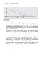
Observing skews: bonds
Figure 20.1 shows a graph of the volatility skew for options on March
Treasury Bonds. Below that, Table 20.1 gives the data containing the
implied volatilities used to plot the skew.

200 Part 3

Thinking about options
Table 20.1 March Treasury Bond options, 87 days until
expiration, March futures at 128.01
Strike Call value Call implied
volatility
Put value Put implied
volatility

112 0.01 11.21
114 0.03 11.47
116 0.06 11.21
118 0.11 10.84
120 0.19 10.38
122 0.33 10.01
124 0.57 9.76
126 3.31 9.57 1.30 9.55
*128 2.22 9.44 2.20 9.43
100 106 112 118 124 130 136 142 148
10
0
Strike v . volatility
Figure 20.1
Options volatility skew: March Treasury Bond, underlying futures
contract at 128.01
Source: pmpublishing.com.

20

Volatility skews 201
Strike Call value Call implied
volatility
Put value Put implied
volatility
130 1.32 9.44 3.29 9.45
132 0.59 9.54
134 0.34 9.58
136 0.20 9.84
138 0.11 9.98

140 0.07 10.45
142 0.04 10.70
144 0.02 10.76
146 0.01 10.86
Source: Data courtesy of pmpublishing.com.
In Figure 20.1, the dotted line is the actual plot of the implieds from strike
to strike, while the solid line has been generated with an algorithm. Some
traders use the equation to determine if an option is undervalued or over-
valued. The discrepancies as you can see are very small.
The ATM implied volatility is that of the 128 strike, at 9.44 per cent.
Note that the implied volatility of the 136 call is 9.84 per cent, while the
implied of the 120 put is 10.38 per cent, and that both these strikes are
equidistant from the money.
Calls and puts of the strike prices ascending from the at-the-money strike
are said to be on the call skew, while calls and puts of the strike prices
descending from the at-the-money strike are said to be on the put skew.
Here, both the call and put skews have increased implieds, and so they are
said to be positive. This type of skew is often found in longer-term debt
markets such as bonds, gilts and bunds.
(Personally, I refer to this type of skew as a ‘parabolic’ skew, because of its
obvious resemblance to a parabola.)

202 Part 3

Thinking about options
Observing skews: stocks and stock indexes
Figure 20.2 shows a graph of the volatility skew for December options on
the OEX. Table 20.2 gives the data containing the implied volatilities used
to plot the skew.
Again, the dotted line is the actual plot of the implieds from strike to

strike, while the solid line has been generated with an algorithm. The close
match-up may seem arbitrary, but because skews continue to exhibit regu-
lar patterns over the years, they are calculable.
The ATM implied volatility is that of the 590 strike, at 17.82 per cent.
Note that the implied volatility of the 610 call is 15.12 per cent, while the
implied of the 570 put is 20.56 per cent, and that both these strikes are
equidistant from the money. Note also that the implied of the 500 strike is
34.46 per cent, or almost double that of the ATM implied.
Here the put skew is positive while the call skew, with decreasing implieds,
is negative. This type of skew is found in other stock index options, such
as the FTSE.
(Personally, I refer to this type of skew as a ‘linear’ skew. It is simply more
linear than a parabolic skew. Note that the tail of the call skew flattens out.)
410 435 460 485 510 535 560 585 610
10
Strike v . volatility
40
50
30
20
Figure 20.2
Options volatility skew: December OEX, underlying index at
587.18, December synthetic future at 590.00
Source: pmpublishing.com.

20

Volatility skews 203
Table 20.2 OEX December options
December OEX options

23 days until expiration
Underlying index at 587.18
December synthetic future at 590.00
Strike Call value Call implied
volatility
Put value Put implied
volatility
420 0.13 53.67
430 0.19 52.77
440 0.25 51.16
450 0.25 47.66
460 0.19 42.59
480 0.31 38.71
490 0.44 37.19
500 0.50 34.46
515 0.81 31.92
545 2.00 25.98
550 2.38 25.06
555 2.75 23.90
570 4.50 20.56
575 21.00 20.75
580 17.13 19.60 6.75 18.87
585 13.50 18.44 8.38 18.21
*590 10.50 17.82 10.50 17.82
595 7.75 16.98
600 5.38 16.06
605 3.63 15.49
610 2.38 15.12
615 1.56 15.05
620 1.00 15.01

630 0.50 15.84
Source: Data courtesy of pmpublishing.com.

204 Part 3

Thinking about options
Volatility skews on individual stocks
Skews on individual stocks have basically the same characteristics as skews
on the indexes. Figure 20.3 shows a recent skew of June options on Marks
and Spencer.
On this day, M&S settled at 375.80.
1
Observing skews: Commodities
Volatility skews in commodities have their own spe-
cial properties. As an example, we can examine the
skew for December 2010 Corn (see Figure 20.4).
1
Figures courtesy of the London International Financial Futures and Options Exchange,
LIFFE.
24
26
28
Implied volatilities
30
32
22
280
300 320 340 360
Strikes
380 400 420 440

Figure 20.3
Recent skew of June options on Marks and Spencer
volatility skews in
commodities have their
own special properties
27
29
31
33
35
37
25
280
300 320 340 360 380 400 420 440 460 480
Figure 20.4
Skew for December 2010 Corn with Corn at $3.80 per bushell

20

Volatility skews 205
Here, we have a typical commodities volatility skew. The call side is posi-
tive because producers and consumers wish to hedge shortage of supply.
They buy calls.
The new skew
Recently we have seen a change in commodities’ skews. Have a look at the
crude oil chart in Figure 20.5.
Here we have a positive put skew. It resembles the skew in stocks and
bonds, not commodities. So what’s going on? Here’s my opinion.
Oil is now being traded by the banks and hedge funds. If you can think
back a few years, then you’ll remember that commodities were a niche

market. They were traded by consumers and producers. This is no longer
the case. Commodities are now an asset class, supposedly.
The result is that the current open interest in derivatives contracts over-
whelms the available supply. The longs outnumber the shorts, and they
have more money. Price is therefore supported. But in order to hedge their
asset, the funds buy puts. That’s why there’s a positive put skew in oil. So,
in the end, what’s going to happen? A blow-out. No firm, no one, no body
is bigger that the market. Think of the Hunt brothers who tried to corner
silver in the 1970s.
29
30
31
32
33
Vols
CL
35
36
37
38
28
6700
6800
6900
7000
7100
7200
7300
7400
7500

7600
7700
7800
7900
8000
8100
8200
8300
8400
8500
8600
8700
Figure 20.5
Crude oil skew

206 Part 3

Thinking about options
Sooner or later, traders – and I mean big ones – will get wise to the weak-
ness of the longs and they will short them. Then the longs will be routed.
In the meantime, you might ask your bank manager if his firm has expo-
sure to commodities.
Trading skews
So how to trade the skews? If there is a positive skew, one suggestion is
to neutralise your exposure by buying the 1 × 1 call spread or put spread.
You’re then financing your long option with a short option that is more
expensive in terms of implied volatility. You’re financing option is value
for money. There is more on this topic below.
Volatility skews versus the at-the-money
implied volatility

Regardless of the nature of the skews, the implied volatility of any options
contract, i.e. the implied that corresponds most closely to the current vola-
tility of the underlying, is always the implied that is at-the-money. One
can say that the at-the-money strike, however that may change, is always
the focal point of both the call and put skews.
Why there are skews
There is no agreement as to why there are skews, apart from the obvious
reason of supply and demand for the options. We know, however, by study-
ing historical data that large price changes in many underlyings occur with
greater frequency than are accounted for by normal distribution. At least
once in a generation an asteroid hits the stock market. Skews might seem
irrational, but then so do many market events.
Don’t make the mistake of thinking that skews exist because brokers like
to buy or sell out-of-the-money options, or because a particular house or
group of houses always buys or sells certain options. One might as well say
that short-term interest rates are at their current levels because the central
banks hold them here.
2
Markets don’t operate in this way; they are more
powerful than the participants.
2
True, central banks have in the past resisted monetary trends, but only by placing their
nations’ economies at risk.

20

Volatility skews 207
For whatever reasons, skews continue to appear in most options contracts
year after year, and they continue to display similar patterns in each con-
tract. Most of us by now have learned to treat them with respect.

I have personal opinions on the reasons for volatility skews. A skew is a
function of variations in implied volatility. Like the implied, it indicates
market expectations for the near-term level of the historical volatility. It
therefore indicates what the market expects the historical volatility will
be if the underlying suddenly shifts to a new level in the direction of the
skew. This is a form of discounting, which all markets do.
Further, a parabolic-shaped, positive skew indicates that the implied is
likely to remain relatively stable when the underlying remains in the cur-
rent trading range. The belly of the skew accounts for this. The increasing
slopes of the parabolic skew indicate that the implied is likely to increase
exponentially if the underlying suddenly moves towards the wings of the
skew and breaks through the current trading range. Again, this is a form of
discounting by the market.
Most stock index and long-term interest rate contracts have positive put
skews because these markets, more often than not, become more volatile
as they break. There is also perennial demand for puts in these markets to
protect against loss of asset value.
Many commodities have positive call skews. Commodities become more
volatile as prices increase, which they suddenly do when faced with supply
shortages. Corn and soybeans have had positive call skews for years. If
drought conditions occur, grain dealers find it difficult to honour forward
commitments. Cash and futures prices, along with the implied volatilities
of options, soar.
A flat or negative skew indicates that the volatility of an underlying is
expected to be stable, or to decline slightly if the underlying moves in its
direction. Bonds spend long periods of time with flat to slightly positive
call skews during periods of interest rate stability. Commodities often have
negative put skews because slackening demand results in their grinding
lower. Negative call skews in stock indexes indicate that as their markets
move steadily higher and the value of their indexes increases, an equiva-

lent price change calculates to a lower historical volatility.

208 Part 3

Thinking about options
Skew behaviour towards expiration
Skews can change their degree of positiveness or negativeness. Positive
skews most often become more positive as they approach expiration.
The underlying contract for this January set of T-Bond options is the same
as for the previous March set of T-Bond options; it is the March futures
contract. Here, the implied of the ATM call at the 128 strike is lower, at
8.14 (see Table 20.4). The implied of the January 122 put is greater,
at 10.42, than the March 122 put at 10.01. The January 134 call has an
implied of 9.19, while the March 134 call has an implied of 9.58. While
both January skews are increased, the put skew exhibits the more radi-
cal change. You may compare the implied volatilities strike by strike (see
Figure 20.6).
117 120 123 126 129 132 135 138
8
Strike v . volatility
11
13
10
9
12
14
15
Figure 20.6
January T-Bond options skew
Source: pmpublishing.com.

20

Volatility skews 209
Table 20.4 January Treasury Bond options
January Treasury Bond options
24 days until expiration
March future at 128.01
Strike Call
value
Call
implied
Call delta Put
value
Put
implied
Put delta
121 0.01 10.02 0.01
122 0.03 10.42 0.03
123 0.05 9.92 0.06
124 0.07 9.00 0.08
125 0.14 8.91 0.14
126 2.26 8.59 0.77 0.25 8.68 0.23
127 1.44 8.44 0.65 0.42 8.42 0.35
*128 1.05 8.14 0.51 1.04 8.26 0.49
129 0.43 8.30 0.36 1.41 8.32 0.63
130 0.25 8.40 0.24 2.23 8.46 0.75
131 0.13 8.38 0.14
132 0.07 8.62 0.09
133 0.04 9.01 0.05

134 0.02 9.19 0.03
135 0.01 9.41 0.01
Source: pmpublishing.com.
Skews’ shift with underlying
Skews most often shift horizontally with the price of their underlying con-
tracts. If an underlying drifts back and forth in a range, the skew will most
often range as well. The focal point clings to the at-the-money strike, with
little change to the ATM implied. This effectively changes the implied of
each strike.

210 Part 3

Thinking about options
For example, if the above March T-Bond contract rose to 129.01 then
the implieds of all the strikes would be likely to shift to the next strike
upward. The January 129 calls would have an implied of 8.14, and the
January 123 puts would have an implied of 10.42, etc.
This occurrence presupposes no change in the historical or ATM implied
volatility. Here the underlying is most often trading in a range. Sometimes
the underlying moves but the focal point of the skew clings to a strike;
this occurs when the market expects a retracement.
Skews’ change of degree
A skew often becomes more positive if the underlying makes a sudden
move, or threatens to make a sudden move, in its direction. A bond market
put skew may become more positive if an inflation report is revealed to be
worse than expected. Several days in advance, the put skew may behave in
the same manner if the report is expected to be worse than expected.
Under these circumstances, the skew becomes more like a skew with fewer
days until expiration. If and when the market’s apprehension subsides, the
skew may return to its former level.

A call skew in a stock index may become less negative to flat in anticipa-
tion of a Christmas or January rally, or an imminent cut in interest rates.
Eventually, the skew will revert to its former position.
Skews’ vertical shift
If the ATM implied increases or decreases, then the skew most often
shifts vertically upward or downward. This effectively raises or lowers the
implied of all strikes because the skew retains its shape. The focal point of
the skew remains at the ATM strike (see Figure 20.7).
Caution
Do not assume that skews foretell directional moves or changes in volatility.
Sometimes they do, but often they do not. A stock’s put skew may be bid
because earnings are expected to be bad. When the earnings are reported,
they may be no worse than expected, the put skew may fall, the stock may
rally and volatility may decline. Likewise, a flat call skew in a bond market
is no indicator that events will continue to be dull and routine. If a shock

20

Volatility skews 211
hits the stock market, a flight to quality and so a flight to bonds may result,
rapidly forcing their call implieds, and their call skews, higher
.
Trading with skews
Volatility skews present additional opportunities
for profit as well as additional risks. They are addi-
tional variables which should be considered when
trading options, especially straight long or short
calls and puts. Their risks are lessened through
spreading. The following paragraphs offer guidelines on how to deal with
some of the more common, but by no means all, market situations. Skew

behaviour varies as much as market behaviour.
As you might expect, there are two basic possibilities to skew trading:
O
buying or selling out-of-the money options on a positive skew
O
buying or selling out-of-the-money options on a negative skew.
Trading options on a positive skew
The purchase of an out-of-the-money option on a positive skew, like the
purchase of any option, profits if the underlying moves in its direction
and/or if the implied increases. If the underlying moves in the option’s
100
36
38
34
24
30
28
26
32
22
20
18
16
XYZ
Increased implied
Decrease
implied
Implied vol
Figure 20.7
Skew vertical shift

Volatility skews present
additional opportunities
for profit as well as
additional risks

212 Part 3

Thinking about options
direction, but meets a support or resistance level, the option profits from
direction but often underperforms. This is because the focal point of the
skew shifts horizontally to the at-the-money strike, causing the implied of
the option effectively to decrease (see Figure 20.8).
With XYZ at 100, the 105 call is purchased at an implied that is above
the at-the-money level, and as the underlying moves to the 105 strike,
the option’s implied effectively decreases from 28 per cent to 20 per cent.
The net result is still a profit if time decay has not been too costly. Note
that the implied of the 100 call and put both increase from 20 per cent to
28 per cent.
For example, suppose you pay 25 (
25
/
64
) for the T-Bond January 130 call
from the set in Table 20.4. You might estimate the profit potential for a
two-point rally in bonds by multiplying two points (128 options ticks)
by the average delta of the call over the course of the move. This average
delta is determined by the delta of the 129 call, at 0.36: 128 × 0.36 = 46
ticks profit. Your estimated new value of the 130 call with bonds at 130 is
46 + 25 =
71

/
64
, or 1.07.
By looking at the 128 call with bonds at 128, you note that the current
ATM call has a value of only 1.05. If the ATM implied remains stable, then
the market is telling you that a 130 call with bonds at 130 will have a
value of 1.05.
Effectively then, for a two-point rally, your 130 call may underperform by
two ticks. In practice, this often happens. The reason for this is that you
95 100 105
XYZ
32
38
30
22
36
34
28
26
24
20
Implied vol
Figure 20.8
Positive skew, right horizontal shift

20

Volatility skews 213
have purchased a call at an implied of 8.40 which will be reduced to 8.14
by a horizontal shift in the volatility skew.

In this case, the underperformance is not a great amount. But if the call
were purchased further up the skew (at a higher strike), and if the skew
were more positive, then the reduction due to a decrease in implied vola-
tility would be greater.
In order to minimise this skew risk, you might instead purchase an out-of-
the-money call spread. Here, you could buy the 130 call and sell the 132
call. As the skew shifts, both implieds decrease.
Another approach is simply to pay 1.05 (
69
/
64
) for the 128 call. Here, as
the market rallies, the shift in the skew causes the implied of your call to
increase. Using the delta of the 127 call at 0.65, your expected profit for
a two-point rally would be 0.65 × 128 = 83. The new value of your call is
estimated at 83 + 69 =
152
/
64
, or 2.24.
You note that the current 126 call has a value of 2.26. This is the expected
value of your 128 call if bonds rally two points. Because the implied of
your call increases from 8.14 to 8.59, your 128 call may, and often will,
outperform by two ticks.
Still another approach is to buy the 128–130 call spread. Here, your
spread’s long strike profits from increased volatility, and your spread’s
short strike profits from decreased volatility.
You can use the preceding data to calculate the effect of a skew shift on
the implieds and values of selected puts. If the underlying breaks, puts on
a positive skew may underperform due to a decrease in their implieds.

Trading options on a linear skew
A long out-of-the-money option on a linear skew, or a skew that is call
negative and put positive, presents a couple of possibilities. As the under-
lying rallies, you might expect the skew to shift horizontally, resulting in
an increase in all the implieds. Often this happens.
In Figure 20.9, as XYZ rallies from 100 to 105, all the calls and puts
increase their implied volatility. Note that the reverse situation often
occurs: an underlying breaks, usually on a retracement, and the skew shifts
to the left, resulting in a decrease in all the implieds.