Báo cáo toán học: " Memory bandwidth-scalable motion estimation for mobile video coding" pot
Bạn đang xem bản rút gọn của tài liệu. Xem và tải ngay bản đầy đủ của tài liệu tại đây (861.06 KB, 11 trang )
RESEARCH Open Access
Memory bandwidth-scalable motion estimation
for mobile video coding
Jui-Hung Hsieh
*
, Wei-Cheng Tai and Tian-Sheuan Chang
*
Abstract
The heavy memory access of motion estimation (ME) execution consumes significant power and could limit ME
execution when the available memory bandwidth (BW) is reduced because of access congestion or changes in the
dynamics of the power environment of modern mobile devices. In order to adapt to the changing BW while
maintaining the rate-distortion (R-D) performance, this article proposes a novel data BW-scalable algorithm for ME
with mobile multimedia chips. The available BW is modeled in a R-D sense and allocated to fit the dynamic
contents. The simulation result shows 70% BW savings while keeping equivalent R-D perform ance compared with
H.264 reference software for low-motion CIF-sized video. For high-motion sequences, the result shows our
algorithm can better use the available BW to save an average bit rate of up to 13% with up to 0.1-dB PSNR
increase for similar BW usage.
Keywords: motion estimation, memory bandwidth, H.264/AVC
1. Introduction
With the rapid progress o f semiconductor technology,
video coding is becoming popular in modern mobile
devices to provide video services. In these devices,
motion-compensated temporally predictive coding with
motion estimation (ME) not only contr ibutes the most
to the coding efficiency of modern video encoder
designs [1], but also requires large amounts of computa-
tions as well as data bandwidth (BW) [2]. This leads to
severe design challenges for power-limited mobile
devices. In power-limited mobile device, the available
power could be change d dynamically due to low battery
power or dy namic power management , such as dynamic
voltage and frequency scaling [2,3]. In such cases, the
available data B W could be inconsistent with the video
requirements and be lower than expected. Once this
situation occurs, the video coding will be delayed or
forced to drop frames. Either case leads to unwanted
low video quality. This BW constrained problem is get-
ting worse with increasing camera resolution in mobile
devices.
Broadly speaking, the BW-constrained ME problem is
one of the resource constraints. Other resource
constrained designs [2-9] focus on lowering power con-
sumption, with or without rate-distortion (R-D) optimi-
zation [2-5], or adjusting computational complexity with
rate-control like methods [6-9]. He et al. [2] developed a
new R-D analysis framework with a power constraint.
Subsequently, the power-aware designs [3,4] directly
change their search algorithms without R-D optimiza-
tion to predesigned ones to fit a lower power mode.
Chen et al. [5] used a fast algorithm and data reuse to
achieve a power-aware design. Tai et al. [6] proposed a
novel computation-aware scheme to determine the tar-
get amount of computation power allocated to a frame
and allocated this to each block in a computation-dis-
tortion-optimized manner. The computational complex-
ity complexity-aware designs [7-9] used a rate-control
like method to combine complexity constraints into R-D
optimiza tion. The basic assump tion of these approaches
is that there are limited computational resources in
handheld devices b ut sufficient memory BW. This
assumption could easily fail because of dynamic mobile
environment in which videos are coded and decoded at
the same time or because of the dynamic power man-
agement mentioned above.
To solve the above issue, we propose a BW-scalable
ME algorithm to fit the available data BW constraint.
We assume that the data BW are the limited resource
* Correspondence: ;
Department of Electronics Engineering & Institute of Electronics, National
Chiao-Tung University, Hsinchu, Taiwan
Hsieh et al. EURASIP Journal on Advances in Signal Processing 2011, 2011:126
/>© 2011 Hsieh et al; licensee Springer. This is an Open Access ar ticle distributed under the terms of the Creative Commons Attribution
License ( which permits unrestricted use, distribution, and r eproduc tion in any medium,
provided the original work is prope rly cited.
and could be dynamically changed [3]. The available
data BW will be sufficient in full or normal battery
mode and have a higher working frequency. In low bat-
tery or power-saving mode, the available data BW will
be insufficient due to the lower working frequency or
lower voltage supply. With a lower than expected BW
supply, ME computations could fail to meet real-time
constraints or lead to significant R-D performance loss
due to the macroblock (MB) skipping coding. The pro-
posed method predicts and allocates the memory BW
according to its R-D gain (RDG) and the available BW
to model the bandwidth-rate-distortion (B-R-D) beha-
vior of the existing ME algorithm. This B-R-D algorithm
is a rate-control like method for MB MB-based BW
allocation, which maximizes the coding efficiency under
the BW constraint. The simulation results show that the
proposed algorithm can better utilize the BW instead of
wasting it as other designs do, and it can be scaled to
the available BW.
The rest of this article is organized as follows. The
review of related studies is presented in Section 2. In
Section 3, we propose an analytical B-R-D optimized
model. The online R-D optimized BW-scalable ME
scheme is summarized in Section 4. Section 5 presents
the simulation results and comparisons with traditional
approaches. Finally, Section 6 concludes this article.
2. Review of related studies
To solve the computational complexity and data BW
challenges of ME, va rious approaches have be en pro-
posed, such as parallel full search hardware design and
fast ME algorithms.
Full search ME designs han dle the computational
complexity by using parallel processing elements for
matching cost computation [10]. Furthermore, with i ts
search center at (0, 0), it can reduce the data BW by
reusing the overlapped search area, termed Level C data
reuse in [11]. Such a design style is simple to use, but it
will need constant data BW regardless of the video con-
tents. Besides, to meet the Level C data reuse require-
ment, such a design also needs a larger search range
(SR) to cover the possible best matching point due to
the (0, 0) search center [12], which implies a waste of
data BW compared to methods with a search center at
the motion vector (MV) predictor (MVP).
On the other hand, f ast ME a lgorithms only search a
few candidates so that the computational complexity is
lower. To facilitate such searching, most of the fast algo-
rithms adopt the MVP as the search center [13]. In [14],
most of best matching points are around the MVP,
which can cov er over 90% of the best matching points
within ± 8 SR. Thus, it can have a smaller SR and could
have lower data BW even with poor data reuse between
consecutive searches. However, even the fast ME
algorithm still assumes constant and sufficient data BW
support for the required SR. Some designs with a
dynamic SR [15-17] could have even lower data BW
demands by changing the SR according to the content
content-dependent prediction, but they still assume con-
stant and sufficient BW support in the planning of chip
design. Besides, none of the designs can adapt to
dynamic data BWs. Several approaches have tried to
reduce the r equired data BW. Designs in [18,19] use a
cache to maximize the possible data reuse for irregular
search patterns. Bus BW-effective ME designs in [20,21]
lower the BW requirement by red ucing the pixel repre-
sentation from 8 bits to a binary pattern. However,
these designs are only useful for specific search algo-
rithms without a data BW constraint.
In summary, none of above approaches has considered
data BW as a limited reso urce to explore the possibility
of optimizing its usage in an R-D sense. The assumption
that there will be constant and sufficient BW has the
benefit of simplifying the design procedure, and thus, it
is widely used in VLSI hardware design, but it usually
wastes a lot of data BW because only a portion of the
MBs in a high-motion video will need such a large
amount of data. Such data BW waste is a serious pro-
blem for power-limited mobile devices because data
access to DRAM is off-chip access and thus consumes
significant power, which can be as much as the power
consumption of the video chip [22]. As indicated in
[22], the power consumption of external DRAM access
could be up to 50% of the total power consumed by the
video decoding chip. For encoding, this portion will be
larger but is often neglected in the previous design.
Besides, with a dynamically changing BW, the current
approaches with constant and sufficient BW ass umption
would have insufficient BW for coding, could need
more time to complete the coding and fail the real-time
constraint or drop MB coding and quality to fulfill the
timing constraint. Both situations are not acceptable to
attain a high-quality visual experience.
3. Analytical B-R-D optimized modeling
For a given video coding distortion (or equivalent pic-
ture quality), D, and bit rate, R, if we decrease the avail-
able encoding BW, the coding will generate more
distortion and bits, which in turn implies a higher D
and R for ME operation and more data BW for video
coding. Therefore, the overall BW usage of a ME mod-
ule is linearly proportional to its search area. We intro-
duce a set of BW control parameters, B =[b
1
,b
2
, ,b
L
],
to control the search area of the ME module. The
model with the BW control parameters is of a more
generic form and captures the available data BW under
different system conditions. Consequently, the ME SR
selection is then a function of these control parameters,
Hsieh et al. EURASIP Journal on Advances in Signal Processing 2011, 2011:126
/>Page 2 of 11
denoted by SR( b
1
,b
2
, ,b
L
). However, the overall BW
usage of a ME module is linearly proportional to its
search area. Within the BW-limited design framework,
the encoder BW requirement, denoted by BW, is a func-
tion of SR, and is also a function of B, denoted by
BW =
(
SR
)
= BW(β
1
, β
2
, , β
L
)
(1)
where F(·) is the SR selection model of the ME mod-
ule. To optimize the BW usage, the available data BW,
b
i
, should dynamically be allocated among the MBs
according to their motion characte ristics. Thus, we exe-
cute the ME algorithm with a different SR of BW con-
trol parameters and obtain the corresponding R-D data.
According to our measurements and analysis, the R-D
performance model can well be approximated by the
following expression, denoted by RDG(BW(b
1
,b
2
, ,b
L
))
as (2).
RDG
(
BW
)
= RDG(BW(β
1
, β
2
, , β
L
))
(2)
where
RDG = RDC
init
− RDC
BMA
(3)
and the RDG isthedifferenceoftheLagrangeR-D
cost (RDC)attheMVP(RDC
init
)andthefinalbest
matching position (RDC
BMA
). The Lagrange RDC func-
tion is frequently employed as a measure of ME effi-
ciency, which is defined as
RDC
motion
(
mv, λ
motion
)
= min
SAD
(
s, c
(
mv
))
+ λ
motion
R
mv − pmv
(4)
where mv is the MV received by the ME , and l
motion
indicates the Lagrange multip lier. The distortion term
SAD(s, c(mv)) is the sum of the absolute differences
between the original signal s and the coded video signal
c. The rate term, l
motion
R(mv - pmv ), represents the
motion information and the coded bit length of the MV
difference (MVD) b etween the MV and predicted MV.
Note that Equation 2 is computationally intensive and is
intended for offline analysis to obtain the B-R-D model.
Next, we optimally configure the BW control para-
meters to maximize the video quality (or minimize the
video distortion) and minimize the video bit rate under
the BW constraint. Mathematically, this can be formu-
lated as in (5).
max
{
β
1
,β
2
, β
L
}
RDG = RDG(BW(β
1
, β
2
, , β
L
))
s.t. BW(β
1
, β
2
, β
L
) ≤ BW
(5)
where BW is the available BW pool for video encod-
ing. The optimum solution, denoted by RDG(BW),
describes the B-R-D behavior of the video encoder. The
corresponding optimum BW control parameters are
denoted by {b
i
*(BW)}, 1 ≤ i ≤ L.
More specifically, we develop an analytical B-R-D
model to perform on-line BW optimization for real-time
video coding. For the simplicity of on-line execution,
the RDG formulation can be well approximated by the
following expression.
RDC
init
− RDC
BMA
= γ × BW(β
1
, β
2
, , β
L
)
(6)
where g is a positive constant. In this study, we refer
to BW as the maximum required data BW for ME.
4. Online R-D optimized BW-scalable ME
Section 3 provides a theoretical analysis of the data BW-
limited performance of the B-R-D optimization. How-
ever, in this section, we discuss how this theoretical lim-
ited data BW performance can be realized in practical
video coding. There are four major issues that need to
be addressed. First, the real BW calculation requires glo-
bal knowledge of the on-chip SRAM buffer resource and
reuse strategy. Second, in BW variations between video
coding and decoding as discussed in this section, we
assume that the available data BW for video coding are
time-varying because of non-stationary video input on
the real-time coding and decoding side. Third, once the
optimum BW efficiency of the previous coded MB is
determined, we need to develop a scheme to allocate
and predict the BW interval to achieve the video
smoothness constraint. This approach is computation-
ally intensive and its correspon ding parameter adjust-
ment is only suitable for offline analysis. In real-time
video encoding on mobile devices, it is desirable to
develop a low-complexity scheme that is able to esti-
mate the BW interval paramet ers from the frame statis-
tics collected in the video coding. F ourth, to avoid
under- or over-use of the BW pool, the target SR is
further refined by the neighboring MV. In the following,
we will discuss these issues.
4.1. BW budget initialization
First, the BW budget (BW
budget
)isinitializedforBW
allocation of the overall data BW pool later in the cod-
ing process. This initializa tion takes the available system
BWandconvertsittoadefaultsystemSRfortheME.
Then, the BW budget is allocated with the above system
SR for a GOP, as in (7).
BW
budget
=
BW
Bus
Frame Rate
× GOP
size
(7)
where the BW
Bus
denotes the bus data transmission
rate (bytes/s), Frame_Rate is the num ber of coded
frames per second, and GOP_size denotes the frame
numbers in a GOP. Larger GOP size allows for more
freedom in adjusting the BW. For the purposes of hav-
ing a concrete example that represents common
Hsieh et al. EURASIP Journal on Advances in Signal Processing 2011, 2011:126
/>Page 3 of 11
practices in video coding, the BW budget for the GOP is
set 16 frames in this article.
4.2. BW evaluation in an R-D sense
To justify the BW usage from (6), the BW efficiency,
G
ave
, is defined as the sum of the RDG before the cur-
rent coded k t h MB divided by the total used BW
(
BW
k
usage
), which denotes the accumulated used data
BW up to the (k - 1)th MB, as in (8) and (9).
G
ave
=
k−1
i=1
RDC
i
init
− RDC
i
BMA
BW
k
usage
(8)
where
BW
k
usage
=
k−1
i=1
BW
i
usage
(9)
and
RDC
i
init
denotes the RDC at the predicted MV
position.
RDC
i
BMA
denotes the RDC after the motion
search of the block-matching algorithm, and
BW
k
usage
denot es the used data BW in the ith MB with a Leve l C
data reuse scheme.
G
ave
measures the BW efficiency by averaging the
RDG over the used BW before the kth MB, which
implies how much RDG can be achieved with a unit of
data BW. Thus, the more G
ave
we gain, the better BW
and coding efficiency we will obtain. In the following
step, we will use G
ave
for BW prediction.
4.3. BW prediction and allocation with the smoothness
constraint
With the BW efficiency, G
ave
, we can derive the allowed
BW interval with the BW prediction and allocation. The
BW prediction predicts the available BW for the next
coded MB with the smoothness constraint. The smooth-
ness constraint maintains the quality and the smooth-
ness (i.e., similar RDC) between consecutively coded
MBs. With this constraint and the RDG per unit BW
from (8), we can predict the forward and backward BW
usage and thus, constrain the possible BW usage of the
next coded MB.
First, to keep the quality and the sm oothness between
the current and the previous MBs, we use the RDC data
from previous MBs to make further predictions (10).
RDC
k
init
− G
ave
BW
k
BP
=
k−1
i=1
RDC
i
BMA
k − 1
(10)
where BW
BP
denotes the backward BW prediction, as
shown in latter equation. In (10), the left-hand side is
the target RDC of the current MB, and the right-hand
side is the average RDC of the previous MBs. To main-
tain the quality and the smoothness, ideally, the target
RDC of the current MB will be equal to the average
past RDCs. Thus, if we have larger G
ave
, (10) implies
that less BW (i.e., BW
BP
) is needed to maintain a similar
RDG as the previous MBs. Therefore, the backward pre-
diction for the current kth MB can be derived, as in (11)
from (10).
BW
k
BP
=
RDC
k
init
−
k−1
i=1
RDC
i
BMA
k − 1
G
ave
(11)
In contrast to BW
BP
, we define the forward prediction
BW
FP
to keep the quality and smoothness between the
current and the future MBs by adopting BW informa-
tion as in (12).
BW
k
FP
=
BW
budget
−BW
k
usage
n − (k − 1)
(12)
where n is the overall MB numbers in a GOP. Because
we have no knowledge of the future RDG,theforward
prediction, BW
FP
, is set to the remaining BW budget
divided by the remaining MBs in the GOP that are not
coded yet.
These two BW predictions link the BW usage between
the past MBs and the future MBs. Their relationship can
be used to allocate the available BW as follows:
if ( BW
FP
>BW
BP
) { (condition 1)
BW
lower
=BW
BP
+ 0.5 × (BW
FP
-BW
BP
);
BW
upper
=BW
FP
+ 0.25 × (BW
FP
-BW
BP
);
}
else { (condition 2)
BW
lower
= BW
FP
- 0.5 × (BW
BP
- BW
FP
);
BW
upper
= BW
FP
;
}
in which, BW
lower
and BW
upper
are the lower and
upper bounds of the BW usage per MB, respectively.
The parameters, 0.5 and 0.25, are selec ted empirically
and are easy to implement because they are powers of
2. The parameters are obtained from a two-step process.
In the first step, we execute the proposed BW-scalable
ME algorithm with different configurations of para-
meters to obtain the corresponding BW
lower
, BW
upper
,
and R-D data. Note that this step is computationally
intensive and is intended for offline analysis to obtain
BW
lower
, BW
upper
, and the B-R-D model only. Once the
B-R-D model and the BW intervals BW
lower
and BW
up-
per
are established, we perform the second step, which
optimizes the configuration of the BW control para-
meters to maximize the video quality under the system
Hsieh et al. EURASIP Journal on Advances in Signal Processing 2011, 2011:126
/>Page 4 of 11
BW constraint. Meanwhile, the parameters, which are
empirically selected in the following section, are
obtained by the same method . For condition 1, as
shown in Figure 1, BW
BP
is smaller than BW
FP
,which
impl ies that less BW had been allocated to the previous
MBs, and thus, more BW can be allocated to the next
MB.Asaresult,wesetthelowerbound,BW
lower
,
higher than the average BW in the past MBs (equal to
BW
BP
+ 0.5 × (BW
FP
-BW
BP
)), and also set the upper
bound, BW
upper
, higher than the average BW prediction
in the future MB coding (equal to BW
FP
+0.25×
(BW
FP
- BW
BP
)). This larger BW allocation enables bet-
ter quality. In contrast, for condition 2 in Figure 1,
BW
FP
is smaller than or equal to BW
BP
, which implies
that too much BW had been allocated to the previous
MBs, and hence less BW can be allocated to the next
MB. As a result, both bounds should be lower than
BW
FP
to keep the smoothness and quality, and we set
BW
lower
equal to BW
FP
-0.5×(BW
BP
- BW
FP
)andset
BW
upper
equal to BW
FP
.
4.4. SR decision and refinement
Finally, we employ the above available BW interval and
R-D data to make an SR decision for the next MB cod-
ing. The SR decision is div ided into three cases, and the
corresponding SR adjustment coefficient is resolution
independent, as shown in Figure 2. Case 1 is the BW
limited case because the average BW usage of the
previous MBs falls outside the available BW interval
bounded by BW
upper
and BW
lower
.Thus,thecurrentSR
is decreased by 8 if it is larger than BW
upper
or increased
by 8 if it is smaller than BW
lower
for next MB coding.
The average BW usage of the previous MBs falling
inside the a vailable BW interval implies sufficient BW i s
available for R-D optimization. This can be further
divided into two cases, case 2 and case 3. If the RDC (R ×
D
cur
) is larger than a predefined threshold (case 2), the
video has a bad qua lity, and thus, the S R is increased by
16 for be tter quality in the next MB. This threshold is set
empirically to 4 times, the average RDC of the previous
MBs, i.e., 4(R × D
avg
), for coarse-grained refinement of
the quality. However, if the RDC (R × D
cur
)issmaller
than the predefined threshold (case 3), the video has a
quite smooth quality, and thus, the SR is adjusted slightly.
Thus, the SR remains unchanged if the RDG of the cur-
rent MB (RDG
cur
)iswithintheaverageRDG (RDG
avg
)
plus or minus an adaptive offset (i.e., RDC
BMA
/20000
empirically for fine-grained refinement of quality). How-
ever, if the RDG
cur
is smaller than RDG
avg
- offset,the
video is of good enough quality, and thus, the SR is
decreased by 4 to save BW. On the other hand, if the
RDG
cur
is larger than RDG
avg
+ offset, the quality is low,
and the SR is increased by 4 to improve the quality.
The above SR decisions are further refined to avoid
BWwastebyconsideringtheSRvaluesintheadjacent
MBs, as illustrated in Figure 3a. First, we get the
Figure 1 Illustration of the available BW interval determination.
Figure 2 Illustration of the SR decision.
Hsieh et al. EURASIP Journal on Advances in Signal Processing 2011, 2011:126
/>Page 5 of 11
adj acent MVs from the neighboring blocks and the MV
of previous frame on the co-located block, such as
MV
UL
,MV
U
,MV
UR
,MV
L
,andMV
Cur
, shown in Figure
3b. All these MVs are of sub-pel precision. Then, we
compare these five MVs and choose a maximum MV
(max_mv ). After that, we set the available SR value
using this maximum MV. The refined SR, max_a-
vail_SR,is
max avail SR =
⎧
⎪
⎪
⎨
⎪
⎪
⎩
SR
lower
,maxmv ≤ mv
lower
SR
step
× Ceil
max
mv
SR
step
+ SR
offset
, mv
lower
< max mv ≤ mv
upper
SR
upper
,otherwise
(13)
in which the parameters SR
lower
, SR
upper
, SR
step
,and
SR
offset
are resolution dependent. For our simulation, we
set SR
lower
equal to 4 for CIF and 26 for HD (720P)
resolution. Meanwhile, we set SR
upper
, SR
step
,andSR
offset
equal to 32, 4, and 4 for CIF resol ution and equal to 72,
8, and 2 for HD (720P) resolution. Meanwhile, we set
mv
lower
and mv
upper
equal to 2 and 24 for CIF resolution
and 24 and 64 for HD (720P) resolution.
Finally, the SR is selected by choosing the minimum
SR between max_avail_SR and SR from Figure 2, for
MB coding.
4.5. Summary of the algorithm
Figure 4 shows the proposed B-R-D optimized algorithm
that can be combined with existing ME algorithms to
make them BW scalable. This algorithm first models the
available BW with its RDG and then predicts and allo-
cates the BW in an R-D optimized sense to determine
the available SR. The whole algorithm is repeated for all
inter-coded frames in a GOP and consists of four steps,
as described below.
Step 1. Initialization: Create the BW budget from (7)
for all MBs in a GOP.
Step 2. BW evaluation in an R-D sense: Evaluate the
RDG in terms of the consumed BW as shown in (8) and
(9) to model the BW in a R-D sense.
Step 3. BW prediction and allocation with the
smoothness constraint: From the RDG obtained from
step 2 and the available BW, the BW for the next coded
MB is predicted in (10) to (12) and allocated as
described in Section 4.3 to keep the video quality as
smooth as possible using the smoothness constraint.
Step 4. SR decision and refinement: According to
the available BW from step 3, the SR of next coded MB
is determined and refined in (13) for ME execution.
5. Simulation results
5.1. Simulation conditions
The proposed algorithm was implemented in the H.264/
AVC reference software, JM [23], for performance eva-
luation. The simulation conditions are CIF-sized test
sequences with a baseline profile, no R-D optimization,
one reference frame, a full-search algorithm as well as
an Enhanced Predictive Zonal Search (EPZS) algorithm
[24] for ME, IPPP sequences, 30 frames/s, and 16 frames
per GOP. All of the block matching algorithms were
implemented using Visual C++ on a PC with a 2.66
GHz Intel
®
Core™ 2 Duo CPU.
In the following simulations, we classify the correspond-
ing BW conditions into two patterns: a constant data BW
Figure 3 Illustration of the SR refinement. (a) Flowchart of the SR refinement method. (b) The relationship between neighboring blocks and
the current block.
Hsieh et al. EURASIP Journal on Advances in Signal Processing 2011, 2011:126
/>Page 6 of 11
pattern and a variable data BW pattern. Both patterns pro-
vide the same amount of reference block data for the same
SR ±R. However, t he constant data BW pattern will
assume that the available BW is constant and fixed during
ME operations, which in turn assumes that the available
BW is sufficient and implies that the video encoder does
not have a BW constraint during the video encoding pro-
cess. Meanwhile, the variable data BW pattern will assume
that the available BW is variable during ME operations,
which assumes that the available BW is ins uffici ent a nd
impl ies that the video encoder is BW constrained during
the video encoding process. The constant data BW pattern
is the scenario used in traditional ME design, which does
not consider the other components, while the variable
data BW pattern simulates the scenario where th e BW is
changing due to situations like simultaneous coding and
decoding (defined as SCD mode) in a video phone or dif-
ferent low power modes (defined as LP mode) for mobile
applications. The SCD mode assumes the dec oding uses
merged sequences from Stefan, Akiyo, and Football (inter-
leaved high-motion and low-motion sequences) and sets
the sce ne cut at a multiple of 32 frames. With the above
interleaved decoded sequence, the available BW for encod-
ing will change dynamically, as shown in Figure 5a. Figure
5b shows the LP mode with a descending trend in data
BW in a power aware system. In the following simulations,
we assume the SR for the sear ch algorithm is ± R for the
constant data BW pattern R and the variable data BW pat-
tern case.
To show the benefit of the proposed scheme, we
tested three different BW adaption schemes in the fol-
lowing simulations. The first scheme, denoted as fixed-
SR, is for ME without any BW adaption scheme. Thus,
the total BW for ME is equally distributed for all MB
coding , and its SR setting is constant for the entire cod-
ing time. The second scheme, denoted as simple-SR, is
for ME with a simple BW adaption scheme. Its BW
adaption equally distributes the available data BW to all
MBs in a period, as in the fixed-SR case, but the distri-
bution will be changed when the available BW changes.
Thus, its SR adapts as well. This adaption does not con-
sider the used BW or the related R-D information. The
final scheme, denoted as BRD-SR, is the proposed B-R-
D optimized BW-scalable method.
5.2. B-R-D performance evaluation
Tables 1, 2, 3, 4, and 5 show the simulation results for
the constant and variable BW patterns with the different
BW adaption schemes. Figure 6 shows the average BW
per frame for the high-motion Stefan sequence with the
quantization parameter set to 28.
For the constant BW pattern case, T able 1 illustrates
that the full search ME with the proposed BRD-SR
scheme can attain similar quality performance as the
that with the fixed-SR scheme in the low-motion
sequence (Akiyo sequence) and the medium-motion
sequence (Foreman sequence), but with less BW. In
case of low-motion sequence, the proposed algorithm
can save 35-83% of the BW with different SRs. For the
medium-motion sequence, our algorithm can save 4-
45% of the BW. For the high-motion sequence (Stefan
sequence), our algorithm can save an average bit-rate of
up to 13% and increase the PSNR by up to 0.1 dB under
the low SR constraint. Also, the simulation sho ws simi-
lar results as that in the full search algorithm by apply-
ing our proposed algorithm to the fast algorithm, the
EPZS algorithm, which is due to our effective SR adjust-
ment. For a fair comparison, the presented BW has con-
sidered data reuse [11] in the overlapped region
between search point s, and thus, only new data that are
notinthelocalbufferwillbeloadedfromexternal
memory and counted in the BW usage. In summary, the
proposed algorithm can save data BW for the full search
and EPZS algorithms as well.
Initialization
Bandwidth
Evaluation
Bandwidth
Prediction &
Allocation
SR
Decision &
Refinement
Last Frame
in GOP
Yes
No
Input
V
ideo
Figure 4 Flowchart of the B-R-D optimized modeling method.
Hsieh et al. EURASIP Journal on Advances in Signal Processing 2011, 2011:126
/>Page 7 of 11
For the variable BW pattern case, Tables 2 and 3
compare the results between the BRD-SR scheme and
the simple-SR scheme in the SCD and LP modes. All of
these results show t rends in R-D performance and BW
saving similar to those in Table 1. In summary, these
results show our algorithm with B-R-D optimization can
better utilize the BW for ME computation and achieves
better performance than the fixed-SR and simple-SR
schemes.
Table 4 shows the execution-time of the proposed
algorithm and compares it to the fixed-SR scheme with
the constant BW pattern. The results are similar to
those found with the simple-SR scheme in the variable
BW pattern case. Our proposed algorithm slightly
improves execution time. However, the saving is not
directly proportional to BW saving due to the calcula-
tion overhead of the MB-level BW-scalable scheme.
These overheads can be reduced with fu rther software
Figure 5 Variable data BW pattern with ± 8 SR for: (a) the SCD mode and (b) the LP mode.
Hsieh et al. EURASIP Journal on Advances in Signal Processing 2011, 2011:126
/>Page 8 of 11
optimization or better hardware implementation of the
existing ME engine.
Table 5 shows the si mulation results for the HD reso-
lution videos and a comp ariso n of the proposed scheme
with the fixed-SR scheme. The simulation conditions
are three 720P-sized video sequences with a baseline
profile, no R-D optimization, one reference frame, IPPP
sequences, 30 frames/s, and 16 frames per GOP. All of
the simulation results show similar savings to those
found with CIF resolution, which are listed in Table 1.
This proves the applicability of the proposed algorithm
on larger sized video sequences.
Table 1 Performance comparison with the fixed-SR scheme for CIF resolution
Search
algorithm
Sequence Akiyo Foreman Stefan
BW
pattern
ΔBW
(%)
ΔPSNR
(dB)
ΔBit-rate
(%)
ΔBW
(%)
ΔPSNR
(dB)
ΔBit-rate
(%)
ΔBW
(%)
ΔPSNR
(dB)
ΔBit-rate
(%)
FS Const. 8
a
-35.2 -0.02 +0.24 -4.78 -0.02 +1.79 -1.01 +0.10 -13.42
Const. 16
a
-69.8 -0.01 -0.35 -22.07 -0.02 +2.10 -6.04 +0.01 -2.45
Const. 24
a
-82.8 -0.01 -0.45 -43.74 -0.02 +1.99 -17.59 +0.01 -1.21
EPZS Const. 8
a
-31.3 -0.01 +0.07 -3.66 -0.03 +3.21 -0.25 -0.03 +2.12
Const. 16
a
-65.4 -0.01 -0.17 -21.26 -0.03 +2.53 -7.14 -0.04 +3.13
Const. 24
a
-79.8 +0.01 -0.45 -42.95 -0.03 +2.01 -18.75 -0.02 +1.46
a
means constant BW and SR is set within ± 8 and ± 24.
Table 2 Performance comparison with the simple-SR scheme for CIF resolution in the SCD mode
Search
algorithm
Sequence Akiyo Foreman Stefan
BW
pattern
ΔBW
(%)
ΔPSNR
(dB)
ΔBit-rate
(%)
ΔBW
(%)
ΔPSNR
(dB)
ΔBit-rate
(%)
ΔBW
(%)
ΔPSNR
(dB)
ΔBit-rate
(%)
FS Variable 8
a
-37.8 +0.01 +0.17 -12.30 -0.02 +1.98 -1.38 +0.07 -9.83
Variable 16
a
-69.9 0.00 +0.36 -31.03 -0.02 +3.19 -7.29 +0.01 -2.16
Variable 24
a
-82.8 -0.01 -0.34 -45.56 -0.02 +1.69 -19.10 -0.01 -1.13
EPZS Variable 8
a
-33.1 +0.02 -0.15 -11.0 -0.02 +2.64 -0.76 -0.02 +1.17
Variable 16
a
-65.6 +0.01 +0.20 -29.54 -0.02 +2.37 -7.69 -0.03 +2.98
Variable 24
a
-79.8 0.00 -0.09 -44.72 -0.02 +1.90 -20.8 -0.01 +1.58
a
means variable BW and SR is set within ± 8 and ± 24
Table 3 Performance comparison with the simple-SR scheme for CIF resolution in the LP mode
Search
algorithm
Sequence Akiyo Foreman Stefan
BW
pattern
ΔBW
(%)
ΔPSNR
(dB)
ΔBit-rate
(%)
ΔBW
(%)
ΔPSNR
(dB)
ΔBit-rate
(%)
ΔBW
(%)
ΔPSNR
(dB)
ΔBit-rate
(%)
FS Variable 8 -37.9 -0.01 +0.12 -5.05 0.00 +0.10 -3.49 +0.03 -2.83
Variable 16 -70.2 -0.01 +0.34 -30.1 -0.02 +2.43 -16.5 +0.07 -9.29
Variable 24 -83.0 -0.01 +0.04 -51.2 -0.02 +1.20 -32.6 -0.01 +0.04
EPZS Variable 8 -32.9 0.00 -0.01 -3.44 -0.01 +0.37 -2.73 -0.02 +1.42
Variable 16 -65.7 -0.01 -0.13 -27.8 -0.03 +2.84 -16.2 -0.05 +3.35
Variable 24 -79.9 +0.01 -0.11 -49.8 -0.01 +1.49 -32.1 -0.01 +1.25
Table 4 Execution-time comparison with the fixed-SR
scheme for CIF resolution
Search algorithm Sequence Akiyo Foreman Stefan
BW pattern ΔTime (%)
FS Const. 8 +0.45 +0.06 +0.19
Const. 16 -0.57 -0.32 -0.06
Const. 24 -1.94 -0.69 -0.38
EPZS Const. 8 -1.31 -0.26 -0.45
Const. 16 -2.31 -0.90 -0.20
Const. 24 -3.21 -2.43 -0.90
Hsieh et al. EURASIP Journal on Advances in Signal Processing 2011, 2011:126
/>Page 9 of 11
6. Conclusion
In this article, we propose a BW-scalable approach f or
an ME algorithm to maximize the R-D performance
while dynamically all ocating the available BW.
Compared to the traditional methods, our algorithm
could save up to 70% of th e BW with a full-search algo-
rithm and 65% of the BW with the EPZS algorithm with
an average SR size of ± 16 for low-motion CIF
Table 5 Performance comparison with the fixed-SR scheme for 720P resolution.
Search
algorithm
Sequence Station2 Sunflower Tractor
BW
pattern
ΔBW
(%)
ΔPSNR
(dB)
ΔBit-rate
(%)
ΔBW
(%)
ΔPSNR
(dB)
ΔBit-rate
(%)
ΔBW
(%)
ΔPSNR
(dB)
ΔBit-rate
(%)
FS Const. 56
a
-69.64 -0.01 +0.27 -48.98 -0.01 +0.28 -23.86 0.00 -0.11
Const. 64
a
-75.97 0.00 +0.29 -59.09 -0.01 +0.20 -37.97 0.00 +0.06
EPZS Const.
56
a
-69.82 -0.01 -0.06 -49.75 +0.01 -0.2 -26.52 0.00 +0.17
Const. 64
a
-76.15 0.00 -0.26 -59.69 0.00 +0.39 -40.43 0.00 -0.02
a
means variable BW and SR is set within ± 56 and ± 64.
0
500
1000
1500
2000
2
5
00
1
14
27
40
53
66
79
92
105
118
131
144
157
170
183
196
209
222
235
248
261
274
287
BW (Pixel)
Frame
SR Const 8
System BW
Proposed
0
500
1000
1500
2000
2500
3000
1
14
27
40
53
66
79
92
105
118
131
144
157
170
183
196
209
222
235
248
261
274
287
BW (Pixel)
Frame
SR Random 8
System BW
Proposed
0
500
1000
1500
2000
2500
3000
3500
4000
4500
1
14
27
40
53
66
79
92
105
118
131
144
157
170
183
196
209
222
235
248
261
274
287
BW (Pixel)
Frame
SR Const 16
System BW
Proposed
0
1000
2000
3000
4000
5000
6000
7000
1
14
27
40
53
66
79
92
105
118
131
144
157
170
183
196
209
222
235
248
261
274
287
BW (Pixel)
Frame
SR Const 24
System BW
Proposed
0
1000
2000
3000
4000
5000
6000
1
14
27
40
53
66
79
92
105
118
131
144
157
170
183
196
209
222
235
248
261
274
287
BW (Pixel)
Frame
SR Random 16
System BW
Proposed
0
1000
2000
3000
4000
5000
6000
7000
1
14
27
40
53
66
79
92
105
118
131
144
157
170
183
196
209
222
235
248
261
274
287
BW (Pixel)
Frame
SR Random 24
System BW
Proposed
(a)
(b)
(
c
)
(d)
(e)
(f)
Figure 6 Constant BW patterns with SR equal to: (a) ± 8 (b) ± 16 (c) ± 24 and variable BW patterns with SR equal to (d) ± 8 (e) ± 16
(f) ± 24.
Hsieh et al. EURASIP Journal on Advances in Signal Processing 2011, 2011:126
/>Page 10 of 11
resolution sequences. Compared to either the full search
or EPZS algori thm, our propose d algorithm can save up
to 70% of the BW with an SR size of ± 56 for HD
(720P) resolution video. These savings come from
appropriate MB-level BW allocation. In addition, while
coding high-motion sequences, the simulation result
shows our design could save an average bit rate of up to
13% and increase the average PSNR by up to 0.1 dB
with similar BW usage for CIF resolution. The proposed
design can be combined with current ME designs.
Further study can be done by incorporating this work
into the rate-control scheme or other resource con-
strained algorithms for better performance.
Abbreviations
B-R-D: bandwidth-rate-distortion; BW: bandwidth; BW
BP
: data bandwidth
backward prediction; BWbudget: bandwidth budget; BW
FP
: data bandwidth
forward prediction; EPZS: enhanced predictive zonal search; max_mv:
maximum motion vector; MB: macroblock; MBs: macroblocks; ME: motion
estimation; MV: motion vector; MVD: motion vector difference; MVP: motion
vector predictor; R-D: rate-distortion; RDC: Lagrange R-D cost; RDC
BMA
:
Lagrange R-D cost at the final best matching position; RDC
init
: Lagrange R-D
cost at MVP; RDG: rate-distortion gain; SR: search range.
Acknowledgements
The authors appreciate the anonymous referees and editor for their valuable
comments and suggestions that lead to the improved version of this article.
Competing interests
The authors declare that they have no competing interests.
Received: 17 March 2011 Accepted: 7 December 2011
Published: 7 December 2011
References
1. T Wiegand, GJ Sullivan, G Bjontegaad, A Luthra, Overview of the H.264/AVC
video coding standard. IEEE Trans Circ Syst Video Technol. 13(7), 560–575
(2003)
2. Z He, Y Liang, L Chen, I Ahmad, D Wu, Power-rate-distortion analysis for
wireless video communication under energy constraints. IEEE Trans Circ
Syst Video Technol. 15(5), 645–658 (2005)
3. CJ Lian, SY Chien, CP Lin, PC Tseng, LG Chen, Power-aware multimedia:
concepts and design perspectives. IEEE Circ Syst Mag. 7(2), 26–34 (2007)
4. YH Chen, TC Chen, LG Chen, Power-scalable algorithm and reconfigurable
macro-block pipelining architecture of H.264 encoder for mobile
application, in Proceedings of IEEE International Conference on Multimedia
and Expo, Ontario, Canada, pp. 281–284 (2006)
5. TC Chen, YH Chen, CY Tsai, SF Tsai, SY Chien, LG Chen, 2.8 to 67.2 mw low-
power and power-aware H.264 encoder for mobile applications, Proceedings
of IEEE Symposium on VLSI Circuits, Kyoto, Japan, pp. 222–223 (2007)
6. PL Tai, SY Huang, CT Liu, JS Wang, Computation-aware scheme for
software-based block motion estimation. IEEE Trans Circ Syst Video Technol.
13(9), 901–913 (2003). doi:10.1109/TCSVT.2003.816510
7. YV Ivanov, CJ Bleakley, Dynamic complexity scaling for real-time H.264/AVC
video encoding, in Proceedings of the 9th International Conference on
Multimedia, Augsburg, Germany, pp. 962–970 (2007)
8. HF Ates, Y Altunbasak, Rate-distortion and complexity optimized motion
estimation for H.264 video coding. IEEE Trans Circ Syst Video Technol. 18(2),
159–171 (2008)
9. CY Chang, JJ Leou, SS Kuo, HY Chen, A new computation-aware scheme
for motion estimation in H.264, in Proceedings of IEEE International
Conference on Computer and Information Technology, Sydney, Australia, pp.
561–565 (2008)
10. JF Shen, TC Wang, LG Chen, A novel low-power full-search block-matching
motion estimation design for H.263+. IEEE Trans Circ Syst Video Technol.
11(7), 890–897 (2001). doi:10.1109/76.931116
11. JC Tuan, TS Chang, CW Jen, On the data reuse and memory bandwidth
analysis for full-search block-matching VLSI architecture. IEEE Trans Circ Syst
Video Technol. 12(1), 61–72 (2002). doi:10.1109/76.981846
12. SS Lin, PC Tseng, LG Chen, Low-power parallel tree architecture for full
search block-matching motion estimation, in Proceedings of IEEE
International Symposium on Circuits and Systems, British Columbia, Canada,
pp. 313–316 (2004)
13. P Kuhn, Algorithms, Complexity Analysis and VLSI Architectures for MPGE-4
Motion Estimation (Kluwer Academic, Norwell, MA, 1999)
14. YK Lin, CC Lin, TY Kuo, TS Chang, A hardware-efficient H.264/AVC motion-
estimation design for high-definition video. IEEE Trans Circ Syst I. 55(6),
1526–1535 (2008)
15. XZ Xu, Y He, Modification of dynamic search range for JVT, in Joint Video
Team, Doc JVT-Q088, (Nice, France, 2005)
16. Z Liu, J Zhou, S Goto, T Ikenaga, Motion estimation optimization for H.264/
AVC using source image edge features. IEEE Trans Circ Syst Video Technol.
19(8), 1095–
1107 (2009)
17. H Shim, CM Kyung, Selective search area reuse algorithm for low external
memory access motion estimation. IEEE Trans Circ Syst Video Technol.
19(7), 1044–1050 (2009)
18. WY Chen, LF Ding, PK Tsung, LG Chen, Algorithm and architecture design
of cache system for motion estimation in high definition H.264/AVC, in
Proceedings of IEEE International Conference on Acoustics, Speech, and Signal
Processing, Las Vegas, USA, pp. 2193–2196 (2008)
19. TC Chen, YH Chen, SF Tsai, SY Chien, LG Chen, Fast algorithm and
architecture design of low-power integer motion estimation for H.264/AVC.
IEEE Trans Circ Syst Video Technol. 17(5), 568–577 (2007)
20. JH Luo, CN Wang, TH Chiang, A novel all-binary motion estimation with
optimized hardware architectures. IEEE Trans Circ Syst Video Technol. 12(8),
700–712 (2002). doi:10.1109/TCSVT.2002.800859
21. SH Wang, SH Tai, TH Chiang, A low-power and bandwidth-efficient motion
estimation IP core design using binary search. IEEE Trans Circ Syst Video
Technol. 19(5), 760–765 (2009)
22. TM Liu, TA Lin, SZ Wang, WP Lee, JY Yang, KC Hou, CY Lee, A 125 μw, fully
scalable MPEG-2 and H.264/AVC video decoder for mobile applications. IEEE
J Solid-State Circ. 42(1), 161–169 (2007)
23. Joint Video Team Reference Software JM12.2, ITU-T />suehring/tml/download/
24. HYC Tourapis, AM Tourapis, Fast motion estimation within the H.264 codec,
in Proceedings of IEEE International Conference on Multimedia and Expo,
Baltimore, USA, pp. 517–520 (2003)
doi:10.1186/1687-6180-2011-126
Cite this article as: Hsieh et al.: Memory bandwidth-scalable motion
estimation for mobile video coding. EURASIP Journal on Advances in
Signal Processing 2011 2011:126.
Submit your manuscript to a
journal and benefi t from:
7 Convenient online submission
7 Rigorous peer review
7 Immediate publication on acceptance
7 Open access: articles freely available online
7 High visibility within the fi eld
7 Retaining the copyright to your article
Submit your next manuscript at 7 springeropen.com
Hsieh et al. EURASIP Journal on Advances in Signal Processing 2011, 2011:126
/>Page 11 of 11