Báo cáo hóa học: " Procedure for the steady-state verification of modulation-based noise reduction systems in hearing instruments" doc

Lamm et al. EURASIP Journal on Advances in Signal Processing 2011, 2011:100
/>
RESEARCH

Open Access

Procedure for the steady-state verification of
modulation-based noise reduction systems in
hearing instruments
Jesko G Lamm*, Anna K Berg, Christian M Künzler, Bernhard Kuenzle and Christian G Glück

Abstract
Hearing instrument verification involves measuring the performance of modulation-based noise reduction systems.
The article proposes a systematic procedure for their verification. The procedure has the potential for application in
the verification of other signal processing systems, because it is independent of the hearing instrument domain. Its
key concept, the separation of abstract and concrete design of test signals, has been adopted from the embedded
systems domain. Specifically for modulation-based noise reduction systems in hearing instruments, the article
shows a complete implementation of the verification procedure, proposing improvements of existing
measurement techniques. To fully cover the verification procedure, a new measurement approach based on
maximum length sequences and DFT processing is introduced, revisiting concepts of system identification that
came up in the 1970s. These can easily be used with the computational resources of today’s microcomputers.
Sample measurements with existing hearing instruments demonstrate the verification procedure with different
measurement techniques.
1 Introduction
A hearing instrument should assist its user by amplifying
sound with a certain gain, but can also cause discomfort
in noisy environments. Therefore, its noise reduction
subsystem should reduce the hearing instrument’s gain
while noise is present - usually dependent on frequency
in different subbands. To preserve speech understanding,
the noise reduction should avoid gain reduction in those

subbands that contain speech. Based on the observation
that speech has a characteristic modulation spectrum [1],
a modulation-based noise reduction should detect speech
by its modulation [2], which is the fluctuation of a subband signal’s envelope over time. As a consequence,
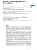
modulation-based noise reduction will reduce gain more
strongly in a subband carrying unmodulated sound than
in a subband with modulated sound [3], as it has been
illustrated in Figure 1.
This article describes the verification of a noise reduction subsystem within the fully integrated hearing
instrument. By verification we mean the confirmation of
* Correspondence:
Bernafon AG, Morgenstrasse 131, 3018 Bern, Switzerland JGL: EURASIP
Member

compliance with the specified requirements, here, by
measurement. This means that the scope of this article
is limited to the measurement of system responses
rather than a clinical verification of the noise reduction
functionality under test.
Measuring system responses with test signals is a typical problem of system identification and has been solved
with measurement techniques based on test signals that
meet some typical requirements regarding their power
spectrum and their amplitude distribution. Particularly,
the minimization of peaks has been of interest with
regard to the fact that practical systems have a limited
dynamic range. However, the synthesis of test signals
that allow enforcing a signal feature like modulation has
only recently been proposed [4,5].
This article puts the synthesis techniques of prior
work into the context of systematic verification, focusing

the so-called coverage of the system’s input parameters.
We show how to systematically design sets of test signals that drive the system under test into a number of
different states, allowing to confirm a complete verification of the subsystem of interest.
A process for achieving the systematic verification is
needed. While processes targeted at test coverage have

© 2011 Lamm et al; licensee Springer. This is an Open Access article distributed under the terms of the Creative Commons Attribution
License ( which permits unrestricted use, distribution, and reproduction in any medium,
provided the original work is properly cited.


Lamm et al. EURASIP Journal on Advances in Signal Processing 2011, 2011:100
/>
Page 2 of 20

Figure 1 The gain reduction (attenuation) of a modulation-based noise reduction system is strongest for low modulation depth. Figure
based on [3].

been described for the verification of purely softwareoriented systems (e.g., [6]) or simple signal processing
systems like e.g., control units in automotive technology
([7,8]), there has not yet been such work for systems
that should provide intense digital signal processing, like
e.g., noise reduction subsystems in hearing instruments.
This article introduces test design techniques for signal processing systems by combining existing test processes from the embedded systems domain with signal
design techniques from system identification into a
novel verification procedure. Its key concept is to obtain
an abstract description of test sequences first, in order
to derive concrete test signals in a second step. Since
these will have to be synthetic in order to match the criteria defined by the test sequence, they are not suitable
for testing the system under realistic conditions.

It is therefore a prerequisite for the procedure to have
requirements toward the system under test stated in a
technical, measurable way. A typical application is the
regression testing in product development where the
performance characteristics of the system under development are re-assessed after implementation changes.
Typically, additional tests under realistic conditions (e.g.,
a clinical trial) are needed before a product can be
released, but these are out of scope of the presented
procedure.
We believe that the verification procedure is applicable to different kinds of signal processing systems,
because one of its essential parts-the abstract description of test signals that can be implemented with

different synthesis techniques-is independent of the kind
of application, but also because applications other than
hearing instruments have to deal with subsystems similar to a noise reduction, e.g., being based on signal features (like e.g., music classification for portable devices
[9]) or having to adapt their processing based on information encoded in the signal (like e.g., voice activitydependent transmission systems in telephony [10]).
Therefore the procedure itself will be described independently of our application area, hearing instruments.
After introducing definitions of terms and concepts as
well as the proposed verification procedure, the article
will report experiments demonstrating the procedure
with modulation-based noise reduction subsystems of
hearing instruments. In contrast to previously reported
measurements for verifying these [4,5,11,12], the ones
presented here are based on a design for test coverage
that is derived from the requirements toward the subsystem under test.

2 Definitions
2.1 Definitions related to signal processing
2.1.1 Signals

This section defines different kinds of signals to be used
in measurements.
• A signal whose amplitude has only two discrete
values is called a binary signal.
• A perfect sequence is a stimulus whose spectral
components are constant over the whole Nyquist


Lamm et al. EURASIP Journal on Advances in Signal Processing 2011, 2011:100
/>
frequency range (see e.g., [13] for a more formal
definition of a perfect sequence).
2.1.2 Frequency response measurements

This section defines different ways of measuring frequency responses of the system or one of its subsystems.
They are based on digital signal processing and thus
assume that test stimuli and the output signal of the
system under test are available as digital waveforms, as
shown in Figure 2 where one digital waveform x enters
the system under test and another one, y, is its output
signal. For systems with analog transducers like hearing
instruments, the signals x and y have to be interfaced to
the system under test via a digital-to-analog and an analog-to-digital converter. This is omitted for simplicity in
Figure 2.
NLMS-based measurement As an improvement of the
least mean squares (LMS) algorithm that has been introduced by Widrow and Hoff [14], Nagumo and Noda
[15] have introduced the normalized least mean squares
(NLMS) algorithm. It iteratively approximates the
impulse response h(n) of the system under test with tap
weight factors ĥ (n) of an adaptive filter whose frequency response can be used as an estimate of the system’s frequency response H(f).

DFT-based measurements Processing the signals x and
y with the Discrete Fourier Transform (DFT) can
approximate the frequency response function H(f) of the
system h(n) [16,17]. For the specification of the detailed

Page 3 of 20

computation, let the frequency bin number k of the
DFT of one frame of signal x at discrete time n be Xn
(k). Let Yn(k) be the according value of signal y. Then,
the corresponding frequency bin Hn(k) of the approximated frequency response is given by the equation
below.
Hn (k) =

Yn (k)
Xn (k)

(1)

Differential measurements Observing the frequency
response of one of a linear system’s subsystems is possible by differential measurements [4], i.e., a combination
of two separate measurements with an identical stimulus, once with the subsystem of interest activated and
once having it deactivated. Dividing the frequency
responses of both measurements can show the effect of
the subsystem of interest on the frequency response of
the whole system.
2.1.3 Modulation/modulation frequency

The modulation definition from the introduction was
based on the signal envelope, which is often used in

quantifying modulation (e.g., as the basis of the modulation spectrum like in [1]) and shall therefore also be
used here as a basis of a first definition related to modulation: from the observation of signal envelope within
one time frame let the observed minimum be the modulation valley, and let the maximum be the modulation
peak accordingly. We use m Ỵ [Mmin, Mmax] to denote

Figure 2 Definition of operators and signals involved in frequency response approximation.


Lamm et al. EURASIP Journal on Advances in Signal Processing 2011, 2011:100
/>
the modulation depth and define:
m/dB = 10 · log10

signal power at modulation peaks
. (2)
signal power at modulation valleys

This definition is a good basis for developing hearing
instruments and is also valid for the samples used in the
experimental part of this article; however, it is undefined
if the denominator becomes zero, it relates to only one
time frame and is furthermore dependent on time constants of envelope estimators and power estimators,
which are usually not specified in the data sheet of a
hearing instrument. For the construction of synthetic
stimuli, we therefore propose another approach for
defining the modulation depth: for a given subband with
index b, we define the corresponding modulation depth
mb indirectly, by describing a reference signal that has
this modulation depth. To describe this signal, we first
need an auxiliary signal μb that is fully modulated by a

cosine term. It is given by the equation below.
μb (n, fm,b ) =

2
fm,b
n + ϕb
· 1 + cos 2π
3
fs

· λb (n). (3)

Here, n is the sample index, fs is the sampling rate, fm,
is the modulation frequency in subband b, and lb is a
band-limited stationary signal with a constant envelope
over time (which can in some cases only be approximated, but is indeed achieved with the binary signals we
will discuss later). Considerations on the signal’s band
limits will follow further below.
Using the auxiliary signal μb, the reference signal, sb,
can be constructed, as described by the equation below.

b

σb (n, fm,b ) = ab · μb (n, fm,b ) + (1 − ab ) · υb (n).

(4)

Here, the signal νb is again a band-limited stationary
signal with constant envelope and shall have the same
RMS as the signal lb, and the factor ab is the link to the

modulation depth via the following equation:
⎧
1
⎨
−
(mb /dB)
(5)
ab = 1 − 10 20
; mb < Mmax
⎩
1
; mb = Mmax
2.2 Definitions related to verification

• Test coverage would ideally describe the percentage
of the system’s input or state parameter range used
during tests. In the case of a signal processing system dealing with quasi-continuous signals, the range
of possible input signals is dramatically large and has
to be constrained to a moderate number of test signals for practical testing. The selection of tests is
here based on the hypothesis that one test signal
from a certain class - an equivalence class - is

Page 4 of 20

sufficient to test the whole class. This hypothesis
shall be called uniformity hypothesis [18] in the following. Test coverage in the context of this article
denotes the percentage of equivalence classes rather
than the percentage of possible signals that is
reached by the test. State space coverage is not
considered.

• A test step is a time interval during a test (definition based on [8]).
• A test sequence is a composition of test steps that
cover certain equivalence classes, optionally together
with a specification of transitions between them. Note
that for simplicity, this article does not distinguish
between test sequences and test cases, as does [8].

3 Verification procedure
The procedure is applicable to signal processing systems
that can be characterized by observing their output in
dependency of systematically chosen input signals. The
procedure has three steps to be described in the following sections:
1) Identifying the requirements against which to test
2) Designing tests
3) Performing tests
3.1 Identifying requirements against which to test

Requirements engineering (e.g., [19]) typically ensures
that testable requirements are available. However, this
matter will not be covered here in more detail, because
it is not actually relevant for this article how the
requirements specification has been established. Here, it
is important to have such a specification and, based on
it, identify those requirements that are within the scope
of the test.
3.2 Designing tests
3.2.1 Describing abstract test sequences with regard to test
coverage

Test design should use a method that can ensure the

desired test coverage. In the domain of signal processing
systems, we propose the classification tree method for
embedded systems (CT/ES) from [7,8]: the input
domain of the system under test is partitioned into
equivalence classes according to the original classification tree method from [20], then test sequences are
defined in order to cover them with test steps that are
abstract, i.e., independent of concrete test signals.
Finding suitable equivalence classes is a key to an
appropriate test design; therefore a good starting point
is helpful. We expect the identified requirements
according to Sect. 3.1 to be a suitable starting point,
because they may give hints about the most important
input parameters that have to be considered in


Lamm et al. EURASIP Journal on Advances in Signal Processing 2011, 2011:100
/>
partitioning the system’s input domain. A main reason
for this: we expect the main functionality of the signal
processing systems targeted here to be a processing of
input signals. The requirements thus have to specify
how these input signals have to be processed and thus
make statements about the system’s input domain.
The classification tree representation of equivalence
classes, test sequences and test steps enables the assessment of test coverage and the further elaboration on the
test, i.e., the verification of the test design and the
synthesis of concrete stimuli that comply to it by covering the corresponding equivalence classes of the system’s input space.
It may not be possible to have the classification tree
method cover all system parameters specified by the
requirements according to Sect. 3.1. Therefore the test

designer should also identify those tests that are needed
in addition to the ones from the identified test
sequences in order to verify each requirement with at
least one test.
3.2.2 Selecting the synthesis procedure for implementing
the concrete test signals

This section discusses different stimuli from system
identification and their use as a basis for synthesizing
concrete test signals that match the abstract signal
description as to the previous section. These signals
should be designed for real systems whose usable signal
range has its lower limit in a noise floor and its upper
limit at a certain maximum level that is given by limited
word lengths in the digital domain and/or limited amplitudes in the analog domain. Ideal stimuli would therefore have a white power spectrum, such that the
spectral components of the background noise are negligible compared to those of the stimulus at any frequency. To provide good signal-to-noise performance
within the given level limitations, the peak factor [21] of
the stimulus should also be small. Obviously, binary signals have a minimum peak factor, but are reported to
oppose challenges to some digital-to-analog converters
[22] and cannot match every given power spectrum.
Therefore, different kinds of signals will be considered
in the following.
• Discrete-interval binary signals [23,24] result from
algorithms that search a certain set of continuoustime binary signals for those ones whose power
spectrum approximately matches a specified one.
We define that a discrete-interval binary sequence
(DIBS) is the discrete-time representation of a discrete-interval binary signal.
• Binary maximum length sequences (binary msequences) contain all possible sequences of storage
initialization in a binary shift register of length L,
except the initialization of all storages with zero -

Page 5 of 20

resulting in a sequence length of 2L-1 [22]. For system identification they are usually synthesized with
computer programs [25,26] rather than with shift
registers. Binary m-sequences are perfect sequences
and have a minimum peak factor.
• A periodic multi-sine signal with a predefined discrete power spectrum can be obtained by adding
sine waves of different frequencies. Their amplitudes
result from the desired spectrum; phases, however,
can be varied, e.g., for minimizing the signal’s peak
factor [21,23,27,28]. Signal synthesis is most efficiently done using Fast Fourier Transform methods
[29,30].
While DIBS are based on iterative approximation of the
desired power spectrum, the synthesis of multi-sine signals usually presets the amplitude spectrum and bases its
optimizations on varying the phase. As a consequence,
the synthesis of multi-sine signals usually reaches the
desired power spectrum quite precisely, whereas DIBS
can lack precision, particularly regarding the synthesis of
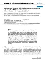
band-limited signals. Figure 3 illustrates this in showing
the spectrum level of a DIBS that has been synthesized
according to the prescription of a band-limited white
power spectrum in the band limits of a typical noise
reduction subband around 1 kHz. The signal indeed has
an approximately white power spectrum in this subband,
but around 4 kHz there is a high amount of side-lobe
energy, as indicated by the arrow in Figure 3.
Sect. 4.5 exemplarily demonstrates the different stimuli that have been described with sample measurements. Their performance in these measurements will
be discussed in Sect. 4.6. A more general discussion of
stimuli can be found in the literature of system identification (e.g., [29]).

3.2.3 Selecting the measurement technique

There are different techniques for measuring the frequency response H(f) of the system under test: for example, the measurement based on the adaptive LMS
algorithm (Figure 2 bottom left) of H(f) and the straightforward computation of an estimate of H(f) from the signals x and y based on the DFT (Figure 2 bottom right).
The impulse response of a system under test can be
time varying and it may be desired to track the corresponding variations over time. The NLMS algorithm
can achieve this under certain conditions and is therefore a common choice in transfer function measurements (e.g., [13]).
The DFT-based measurements require a steady-state
condition of the system under test. The used test signals
should have spectral components that are constant [16]
over the frequency range of interest. They should also
be periodic [4], which can avoid leakage errors [31] in
processing based on the DFT, if the DFT window length


Lamm et al. EURASIP Journal on Advances in Signal Processing 2011, 2011:100
/>
Page 6 of 20

Gain / dB

−20

−40

−60

−80

500

1000
2000
Frequency / Hz

Figure 3 Spectrum level of a sample DIBS.

is a multiple of the period length [29]. If this match of
lengths is not possible, zero stuffing - the insertion of
additional zeros into the DFT frame - can adjust the signal frame to the DFT frame. It has been shown, however, that this may reduce the measurement precision
compared to a situation with matched lengths [32]. As a
consequence, it shall be a prerequisite for all further
considerations about DFT-based processing that the
DFT window length matches the period length of the
used stimulus. In case of signals whose length is not a
power of two, this may mean that the Fast Fourier
Transform algorithm cannot be used. Even in these
cases, we expect the computation time to be sufficiently
short, based on the assumption that measurement data
will be post-processed with the computational power of
a modern desktop computer.
Both LMS-based and DFT-based measurements ideally
need stimuli with a white power spectrum. The DFTbased measurements only have optimum precision when
used with periodic stimuli, whereas the LMS does not
require periodicity of signals. The most important criterion for selecting the measurement approach is the time
variance of the system under test: while LMS-based
measurements can handle time variance under certain
conditions, the DFT-based measurements only work
with a time-invariant system. DFT-based measurements
have the advantage that no convergence of an iterative

algorithm is needed. This makes the measurement window for a given frequency resolution small and thus the
time resolution high.
3.3 Performing tests

How to perform the tests is dependent on the chosen
test design. We can therefore not state a general flow of

activities for this part of the procedure. We rather use
typical experiments to demonstrate the step of performing tests. This will be done within the next section.

4 Measurements
This section demonstrates the application of the verification procedure in the hearing instrument domain,
based on experiments with hearing instruments. The
design of experiments is given by the proposed verification procedure. The device under test and the measurement setup will be presented in the following sections.
4.1 Device under test

In all experiments, the device under test was a hearing
instrument with a modulation-based noise reduction
subsystem. Most of the devices used for the experiments
below were part of recent test plans at the Bernafon
laboratories, allowing us to perform most of the shown
experiments within the regular test plans of the laboratory. As a consequence, different experiments have been
performed with different hearing instrument models,
because test plans do not necessarily foresee to sequentially perform all test cases with the same one. The
noise reduction subsystems of the used hearing instruments were equivalent and thus satisfy the same
requirements and design.
The requirements toward the noise reduction subsystem under test have been stated in Table 1, using “shall”
clauses, which are a common practice in requirements
engineering [19]. Table 1 identifies each of them with a
unique code (ID) to be used for further reference in this

article, but also to show the hierarchy of requirements
(e.g., requirement 1.1.1 adds more detail to requirement
1.1). Literature references in the rightmost column of


Lamm et al. EURASIP Journal on Advances in Signal Processing 2011, 2011:100
/>
Page 7 of 20

Table 1 Requirements toward the noise reduction subsystem
ID

Text

1

The noise reduction shall apply attenuation

Ref.

1.1

Attenuation shall depend on modulation

1.1.1 The dependency between modulation depth (m) and attenuation (a) shall be as follows:

⎧
⎪ A0
⎪
⎨

m − M1
a
= A0 · 1 −
dB ⎪
M2 − M1
⎪
⎩
0

[3,12]

; m ≤ M1
; m ∈]M1 , M2 [
; else

(See Figure 1)
1.1.2 The noise reduction shall be sensitive to modulation frequencies in range [1-12 Hz]

[1]

1.2

[3]

Attenuation shall be applied in individual subbands

1.2.1 The crossover frequencies shall be { List of frequencies }
1.3 The attenuation by the noise reduction shall be superposed linearly with other attenuations in the system

Table 1 indicate sources of the information contained in

the corresponding requirement.
The design of the investigated noise reduction subsystem is shown in Figure 4:
• The gray blocks compose a functional model of the
noise reduction subsystem in the notation of the
Simulinkđ software.
ã The unfilled blocks indicate the IDs of requirements from Table 1 that are fulfilled by the associated functional blocks.

according to Figure 1. This attenuation will be applied
in block “Apply attenuation” together with other
attenuation in the system, which was zero for all experiments except the last one where it resulted from a transient noise reduction system to be described later. The
block “Synchronize” ensures that the signal in the lower
signal path is delayed by the group delay of the upper
path in order to ensure that the processing in block
“Apply attenuation” will be based on correctly timed
information.
4.2 Test setup

The functionality of the noise reduction subsystem
according to Figure 4 is explained in [3] and will only
be briefly summarized here: The block “Filter” extracts
subband contents of the input signal for each subband
individually and feeds these into block “Compute modulation” to estimate modulation depths according to
Equation 2. The block “Compute attenuation” determines attenuation as a function of modulation depth

The setup for performing the designed test consisted of
a combination of off-the-shelf hardware and software as
well as customized computer programs. This section
describes each of them.
4.2.1 Infrastructure for test design

An abstract description of test sequences was done
using the tool CTE® [33,34] that supports the earliermentioned CT/ES method. The MATLAB ® technical

Figure 4 Functional model of a noise reduction subsystem according to [3], annotated with the requirements from Table 1 to be
fulfilled by the different blocks.


Lamm et al. EURASIP Journal on Advances in Signal Processing 2011, 2011:100
/>
computing environment was used to synthesize binary
m-sequences according to [26]. One of its third-party
toolboxes, the Frequency Domain Identification Toolbox
(FDIDENT, [35]), was used for synthesizing discreteinterval binary sequences based on [23] and multi-sine
signals according to [28].
4.2.2 Infrastructure for test execution

For all shown results, the test setup was the same: A
test system was prepared for making measurements
with synthetic test signals. Figure 5 illustrates the setup:
The hearing instrument under test was located in an
off-the-shelf acoustic measurement box with a loudspeaker (L1) for presenting test stimuli to be picked up by
the hearing instrument’s input transducer (M 2 ). The
hearing instrument’s output transducer (L2) was coupled
with a measurement microphone (M 1 ) so tightly that
environment sounds can be neglected in comparison to
the hearing instrument’s output. The coupler is a cavity
that mimics the human ear canal. Here, we used a socalled 2cc-coupler.
Note that the described test setup differs from the
usual condition in which a hearing instrument is worn,
because the effect of the human head on the sound field

from the sound source is not taken into account. The
acoustic effect of the human head in wearing the hearing instrument has thus been neglected here, but it
could easily be modeled by putting the hearing instrument under test on an artificial head within the test box.

Figure 5 Measurement setup.

Page 8 of 20

The test system [36] was implemented using a
National Instruments PXI™ system running customized
computer programs based on National Instruments LabVIEW. The test system was equipped with a NI-PXI
4461 analog input/output card that can play test signals
originating from a hard disk, where they have been
stored after creating them with the MATLAB® technical
computing environment. The signals were presented via
a digital-to-analog converter (D/A) of the input/output
card, an audio amplifier (Amp. A) and the loudspeaker
of the measurement box (L1), while recording the hearing instrument’s output via the measurement microphone (M1), a microphone pre-amplifier (Amp. B) and
an analog-to-digital converter (A/D) of the input/output
card.
The recorded digital data were stored in a file on a
hard disk that could be read by the MATLAB® technical
computing environment for further processing. The
sampling rate for both playing and recording signals was
set to 22,050 Hz. The test system ensured synchronous
playback and recording.
4.3 Test design

Testing a modulation-based noise reduction system
should observe attenuation in different subbands as a

function of modulation. Figure 6 uses the CT/ES method’s proposed graphical notation of classification trees
to show the partitioning of hearing instrument input


Lamm et al. EURASIP Journal on Advances in Signal Processing 2011, 2011:100
/>
Page 9 of 20

Figure 6 Classification Tree representation of the noise reduction test signals. Subbands between number 2 and number B have been
omitted for simplicity.

signals into equivalence classes as a basis for testing a
multi-band noise reduction system with modulationdependency:
• Input parameters (symbolized by rectangles) are
the modulation depths (brief: modulations) in the
different subbands, based on requirement 1.1 and
1.2 in Table 1.
• Equivalence classes (symbolized by range expressions in square brackets) have been derived from
requirement 1.1.1 in Table 1.
• Test sequences ("1”, “2”, “3”,...) and test steps
("1.1”, “1.2”,...) are denoted by short verbal descriptions in the column on the left.
• Filled circles on the grid show that a test step
should cover a certain equivalence class.
• A diagonal straight line between two circles
denotes a gradual transition of the used test signal
between different equivalence classes.
The circles and their connection lines in Figure 6 are
an abstract description of test signals that should be

suited for verifying most multi-band modulation-based

noise reduction systems.
Figure 6 shows two kinds of test sequences: On the one
hand, a static test (1) that covers the extreme modulation
classes of very low and very high modulation for all subbands, and on the other hand dynamic tests (2 to x, one
per subband) that gradually vary modulation within the
intermediate modulation range ]M1, M2[. Together, these
test sequences achieve sufficient test coverage: since all
equivalence classes have at least one circle vertically below
them, all equivalence classes are covered by tests.
The abstract test description from Figure 6 should now
be mapped to concrete test signals that are used for
frequency response measurements based on a suitable
measurement technique. Although NLMS-based measurements are a common way of measuring acoustic frequency
responses (e.g., [13]), we chose DFT-based measurements,
because of the possibility to achieve high time resolution,
which were required in one of the experiments. As a consequence, test signals had to be periodic.
When used as a stimulus for subband measurements,
a periodic test signal needs to have its power


Lamm et al. EURASIP Journal on Advances in Signal Processing 2011, 2011:100
/>
concentrated in the frequency range of interest, and the
most simple assumption is that it should approximate
band-limited white noise. Some synthesis algorithms
require the absolute values of Fourier coefficients of the
signal as an input. If the desired period length in samples is N, and frequency range of interest is from f1 to f2
(where f1 > 0 and f2 ≥ f1+ N-1·fs) and the desired RMS of
the synthesized signal is r, then the target values for the
synthesis algorithm are given by the following absolute

−
values of Fourier coefficients ck (based on [4]):
⎧
⎪
⎪
⎪
⎪
⎪
⎪
⎪
⎨
c =
−
k

⎪
⎪
⎪
⎪
⎪
⎪
⎪
⎩

r
2

f2
N·
fs

;

f1
− N·
fs

0

N · f1
fs

≤ |k| ≤

N · f2
fs

+1
.

(6)

else

Since system tests will acoustically stimulate the system under test, we would theoretically have to describe
acoustic signals here, which are in continuous time.
However, since the native format of the given test system is a digital waveform, we describe signals in discrete
time. All stated sampling rates refer to the test system,
not to the system under test.
Let B be the number of subbands, and let the lower

and upper crossover frequency of subband number b be
fc,b and fc, b+1 respectively. Furthermore, let the signal sb
be the reference signal from Equation 4. The signals in
that equation shall be constructed as follows: the signal
νb shall have a Fourier spectrum that approximates the
one from Equation 6 with f1 = f c,b and f2 = f c,b+1 . The
signal μb be the one from Equation 3 where the signal
lb is synthesized the same way as νb, but with f1 = fc,b +
fm,b and f2 = fc,b+1 - fm,b [4]. Then, the following equation defines a test signal θb that has configurable modulation in subband number b and maximum modulation
in the other subbands:
θb (n) = σb n, fm,b +

μi n, fm,i .

(7)

Page 10 of 20

and 1.3. These requirements can be covered with a simple measurement approach that does not require an
abstract test design. This will be demonstrated in Sect.
4.5.
4.4 Test procedure

For all experiments, the gain in the hearing instrument
under test was set 20 dB below the maximum offered
value to reduce non-linearities. Unless stated differently,
all adaptive features of the hearing instrument, apart
from noise reduction, were turned off for all test runs.
The hearing instrument was furthermore configured for
linear amplification, this means that there was no

dynamic range compression.
Before each experiment, the test system was calibrated
using built-in functionality, in order to ensure that
transfer characteristics of all equipment in the signal
path, particularly the acoustic transducers, were compensated in the digital signal processing of the test system. This ensured that the power spectra encoded in
audio files of the input and output signals were equivalent to the acoustic power spectra at the input and output transducers of the device under test.
According to the earlier-mentioned differential measurement approach, two DFT-based measurements were
performed per stimulus: first with the noise reduction
subsystem of the hearing instrument switched off, and
second while having it switched on.
(on)
Only the output-related DFT spectra Yk (n) of the
(off)
system with noise reduction enabled and Yk (n) of
the system with noise reduction disabled were recorded
to compute the noise reduction s transfer function
(subsystem)
by the following equation that results from
Hk
the definition of the differential measurement in Sect.
2.1.2, from Equation 1 and from the fact that the input
signal was the same for both measurements:

i∈({1,2,...B}\{b})

The parameter b on which the above signal depends
via Equation 3 was left variable to allow for experimenting with different values of it.
The test steps from Figure 6 never require more than
one subband at a time to have a modulation outside the
range [M2, Mmax]. Using only maximum modulation to

cover the equivalence class of that range, one can use the
signal θb from Equation 7 to establish all test steps from
Figure 6, if a suitable modulation of signal sb is chosen in
the one subband whose modulation falls into another
equivalence class (note that for each test step in Figure 6,
there is maximum one definition of such a subband).
So far, the described stimuli therefore cover all
requirements from Table 1, except number 1.1.2, 1.2.1

(on)

(subsystem)

Hk

(n) =

yk

(n)

(off)
Yk (n)

(8)

In using the above equation, measurement samples
(off)
Yk (n)

= 0 would have been treated as invalid samples
and discarded from the result to avoid division by zero,
though in practice, such samples did not occur during
the experiments that were made.
4.5 Experiments
4.5.1 Verification of crossover frequencies

The objective of the test described in this section was
the verification of requirement 1.2.1 from Table 1, thus
to verify the crossover frequencies between the noise


Lamm et al. EURASIP Journal on Advances in Signal Processing 2011, 2011:100
/>
reduction subsystem’s subbands. We separately defined
a signal used for driving the noise reduction subsystem
into a desired state and one used for measuring the system’s frequency response, which - in combination yielded the test signal according to the equation below.
⎧
⎨
s(n) =

⎩

a · sin 2π
p(n)

f0
fm
n + b · 1 + cos 2π n
fs

fs

n
≤T
.
fs
; else

· p(n) ;

(9)

The signal p was chosen to be a periodically repeated
binary m-sequence of 1,023 samples period length, and
the time T that passes between the start of the measurement and the application of the signal p was set to 40s.
The inherent assumption of this procedure is: after time
T the noise reduction subsystem has settled to steady
state and maintains it while the signal s continues, such
that a frequency response can be measured, based on
the stimulus p. The signal applied before time T contains a pure tone to stimulate the noise reduction subband around frequency f0, added to a modulated signal
that is constructed in a way similar to Equation 3. Based
on empirical investigation of the procedure, the parameters a and b were chosen such that the pure tone’s
level was 15 dB higher than the level of the remaining
signal components before time T, in order to make the
unmodulated signal the dominant stimulus around frequency f 0 . The modulation frequency was set to f m =
4Hz, because this is the frequency at which the modulation spectrum of speech has its peak [1].
The frequency f0 was varied stepwise within the bandwidth of the system under test. The step width was chosen between 40 and 250Hz, depending on the
bandwidth of the noise reduction subbands in the given
frequency region.
For each measurement, the signal p(n) was the input

signal of the system under test between time T and
the end of the measurement, allowing for frequency
response measurements. Differential DFT-based measurements were performed to obtain the frequency
response of the noise reduction subsystem immediately
after time T. Averaging of the data resulting from
three subsequent periods of the measurement stimulus
was used for obtaining a smoothed frequency response
[37]. The measured frequency responses were postprocessed by a human observer: it was necessary to
discard duplicate responses of the same subband as
well as invalid measurements that were caused by f 0
inbetween two sub-bands triggering the noise reduction subsystem in both of them. Afterward, the observer could determine crossover frequencies by
graphically intersecting the frequency responses of two
adjacent subbands.
Figure 7 shows some examples of the responses that
were measured. Subfigures a and b show cases in which

Page 11 of 20

more than one noise reduction subband was triggered
by the pure tone of frequency f 0 . The frequency
responses of such cases all had the shown characteristic
shape for the given noise reduction subsystem, allowing
the observer to identify such measurements and ignore
them. Figure 7c, d are examples of valid measurements:
the intersection of their graphs would show that the system under test has a crossover frequency at approximately 1,550 Hz. To result in a passed test, the set of all
obtained frequencies was verified to match specified corner frequencies of the noise reduction sub-bands within
a specified tolerance. Figure 8 shows how the absolute
value of the difference between the specified and the
measured crossover frequency was distributed over eleven valid measurements from the given experiment with
an error-free system under test. The distribution shows

that a typical 10% tolerance band would have resulted in
a passed test, but even a 5% tolerance band would have
been possible in the given case.
4.5.2 Verification of the frequency response for a static
modulation pattern

This section describes the “static test” according to Figure 6, that means a measurement performed with a signal composed of strongly modulated signals with a
modulation depth in range [M2; Mmax] in all subbands
except one - subband number b, in which the modulation is in the range [Mmin; M1]. Based on Sect. 4.3, the
signal θb from Equation 7 was used as the test signal.
The system of equations formed by Equations 7, 3 and
4 was used as the basis for signal synthesis, and the
parameters of these equations were set to ab = 0 (thus
choosing Mmin = 0 as the modulation depth for subband
number b) and fm = 5.4 Hz [4]. The remaining parameter b was varied between the different subbands and
between the different measurements between different
empirically found values. The signals lb and νb in the
resulting equation were synthesized with a level of 70
dB SPL and a period length of 4,096 samples either as
multi-sine signals or as signals of type DIBS. Table 2
lists the measurements that were performed and the
corresponding choice of parameter b and the signal
type of the mentioned signals.
For each measurement, the test stimulus was presented during at least 15 s. Differential measurements of
the noise reduction subsystem’s frequency response
were made, averaging five DFT windows. These windows were taken from the last 5 s of the test run in
order to observe the steady-state condition.
Figure 9 shows the measurement results together with
a reference response (Figure 9a), which has been
obtained by using a functional model of the block

“Apply attenuation” from Figure 4 in the condition in
which it applies zero attenuation to all subbands but b,
and maximally attenuates that subband. The 3 dB


Lamm et al. EURASIP Journal on Advances in Signal Processing 2011, 2011:100
/>
Page 12 of 20

Gain / dB

a
0
−3
−6
500

1000

2000

500

1000

2000

500

1000

2000

500

1000
2000
Frequency / Hz

Gain / dB

b
0
−3
−6

Gain / dB

c
0
−3
−6

Gain / dB

d
0
−3
−6

Figure 7 Determining crossover frequencies of the noise reduction subsystem: (a) f0 = 750 Hz, (b) f0 = 1,000 Hz, (c) f0 = 1,480 Hz, (d) f0 =
1,600 Hz

corner frequencies of the simulated subband b have
been indicated with dashed lines.
Observations: From the measured responses, only the
one of Figure 9d has the correct subband attenuation in

the sense that it produces the expected 3 dB corner frequencies. Furthermore, Figure 9b shows a side effect,
the attenuation in a subband not adjacent to subband
number b (as indicated with an arrow on the figure).


Lamm et al. EURASIP Journal on Advances in Signal Processing 2011, 2011:100
/>
Page 13 of 20

Percentage of occurences

50%
40%

36%
28%

30%

18%

20%

18%

10%
0%

[0%;1%[

[1%;2%[

[2%;3%[

[3%;4%[

Relative deviation of measured frequency from specified frequency
Figure 8 Measured versus specified crossover frequencies.

4.5.3 Investigation of the side effect in the DIBS-based
measurement

Measurement data from different runs of measurement
number 1 according to Table 2 with different hearing
instruments were analyzed in order to investigate the
side effect according to Figure 9b. The hearing instruments had been set to different noise reduction configurations during the measurements. The measurement
data were subdivided according to the sensitivity to
unmodulated noise of the used noise reduction configuration. The higher the configured first knee point “M1“
according to Figure 1, the more sensitivity to unmodulated noise was assumed in the classification. As a result,
three classes were obtained: a “Low” class for low sensitivity, a “Med” class for medium sensitivity, and a
“High” class for high sensitivity.
The data from different runs of the “static test”

according to Figure 6 were plotted in graphs like the
ones of Figure 9, and these were inspected visually. For
each graph, the observer counted frequency bands not
adjacent to subband b whose peak attenuation was more
than 1 dB, thus bands with the side effect according to
Figure 9b. The counted value was divided by the total
number of subbands B, and the result was multiplied by
100, resulting in a percentage of subbands with the side

effect per hearing instrument per class of sensitivity to
unmodulated noise. The results of this analysis are given
in Table 3 for five sample hearing instruments that were
known to have correctly operating noise reduction subsystems from other verification activities not in the
scope of this article. It can be observed that the percentage of side effects increases from the “Low” class to the
“High” class for every observed hearing instrument.
4.5.4 Verification of attenuation with varying modulation

Attenuation function measurements are needed to cover
the “transition tests” according to Figure 6. They should
characterize a modulation-based noise reduction system
by measuring its typical performance characteristic
according to Figure 1. Modulation depth can be varied
by changing parameter ab in Equation 4. This was done
by varying parameter mb in Equation 5 from 0 dB to 20
˜
dB in steps of 2 dB. A test signal θb was constructed as
a modified version of signal θb from Equation 7 and was
used for the measurements. One modification (according to [4]) was to choose a sum index range of ({1, 2,...
B}\{b - 1, b, b + 1}) instead of ({1, 2,... B}\{b}). The subbands that had been removed from the sum index range
were instead targeted with signals of variable modulation according to Equation 4. The modification should

ensure that the stimulus of variable modulation spanned

Table 2 Parametrization of measurements
Choice of parameter i as a function of subband number b

Type of signal lb and νb

1

∀i: i = 0

DIBS

2

∀i: i = 0

Measurement number

3

ϕi =

π
;i = b
2
0 ;i = b

multi-sine
multi-sine

Lamm et al. EURASIP Journal on Advances in Signal Processing 2011, 2011:100
/>
Page 14 of 20

Gain / dB

a
0
−3
−6
500

1000

2000

Gain / dB

b
side effect

0
−3
−6
500

1000

2000

500

1000

2000

500

1000
2000
Frequency / Hz

Gain / dB

c
0
−3
−6

Gain / dB

d
0
−3
−6

Figure 9 Frequency responses of a sample noise reduction subsystem: (a) expected response (simulated), (b), (c), (d) measured response of
measurement #1, #2, #3 respectively

more than one subband of the noise reduction subsystem under test, thus making the procedure invariant to
non-ideal subband split. The mentioned changes are
consistent with the test design (Figure 6), whose

“transition test” sequences do not constrain the modulation of any subband except the one with the specified
variation of modulation depth. Another modification of
˜
signal θb in constructing signal θb was to filter out side


Lamm et al. EURASIP Journal on Advances in Signal Processing 2011, 2011:100
/>
Page 15 of 20

Table 3 Side effects in dependency of modulation sensitivity
Hearing instrument

Percentage of subbands with side effect
in “Low” class (%)

in “Med” class (%)

in “High” class (%)

1

0

0

47

2

0

7

60

3

0

0

60

4

0

7

67

5

0

20

80

lobe influences from the subband of interest [4]: if subband number b is this subband, then one can eliminate
the influences from other subbands by using a bandstop filter whose band limits are outside of subband
number b (here, we chose each of them in the middle of
one subband adjacent to b). Let h be the impulse
response of such a band-stop filter and let “*” be the
˜
convolution operator. Then, θb can be constructed
according to the equation below.
˜
˜
θb (n) = σb (n) + h(n) ∗
i∈({1,2,...B}\{b−1,b,b+1})

μi (n, fm,i ). (10)

Here an auxiliary signal σb was used according to the
˜
following definition:
⎧
;b = 1
⎨ σb (n) + σb+1 (n)
(11)
σb (n) = σb−1 (n) + σb (n)
˜
;b = B .

⎩
σb−1 (n) + σb (n) + σb+1 (n) ; else
The measurement parameters were set like for measurement number 1 from Table 2. For each measurement, the first test signal was presented during at least
15 s. Then, modulation was varied stepwise, as described
above, and for each step, the test signal was presented
long enough to measure in steady-state. Differential

measurements were made, averaging five DFT windows
from the last 5 s of each measurement signal. Attenuation as a function of modulation was extracted from the
measurement data, following a procedure that is given
in [4], which extracts the effective attenuation of subband number b from the measured frequency responses.
The obtained result is shown in Figure 10. The test is
passed, because the figure shows that indeed the
attenuation as a function of modulation depth is
approximately as shown in Figure 1.
4.5.5 Verification of the superposition with transient noise
reduction attenuation

Transient noise reduction systems target a special kind
of noise that has been reported to be one reason for
annoyance among hearing instrument users [38,39]:
non-speech transient noises, i.e., signals with a fast
change of level over time.
Since transient noise reduction systems should act in
addition to traditional noise reduction, they are a good
example for the superposition of additional attenuation
according to requirement 1.3 from Table 1.
This section proposes a test that addresses the stated
requirement. Since the scope of this article is limited to
steady-state responses of modulation-based noise reduction subsystems, we will not cover the verification of a

Attenuation / dB

10

5

0
0

5

10

15

mb / dB
Figure 10 Measured dependency of noise reduction attenuation on modulation depth parameter mb.

20


Lamm et al. EURASIP Journal on Advances in Signal Processing 2011, 2011:100
/>
transient noise reduction subsystem here. Rather, we
show how to test that the traditional noise reduction
subsystem has maintained its steady-state performance
after a short intervention of a superposed transient
noise reduction subsystem.
The challenge here is to insert a transient event into the

test stimulus, but still enabling the observation of the frequency response. Although the given test case looks like a
good application area for time-frequency approaches like
wavelets, we have chosen to stay with the verification techniques that have been presented so far, because we consider the typical mutual exclusion of precise time
resolution and precise frequency resolution in time-frequency techniques as a problem for the given test case.
The approach we propose here operates with absolute
amplitude measurements in the time before and during a
transient noise reduction interaction, and switches to a differential frequency response measurement right afterward.
The test signal s is proposed in the equation below.
⎧
⎪ a · sine(n) + b · 1 + cos 2π fm n
⎪
⎪
⎨
fs
s(n) = c · sine(n)
⎪
⎪
⎪
⎩
p(n)

n
< T1
fs
n
; ∈ [T1 ; T2 ] .
fs
; else

· p(n) ;

(12)

f0
n ; p is a periodically
fs
repeated, 1,023 samples binary m-sequence of 70 dB
SPL, n is the sample index, fs is the sampling rate, f0 is
the frequency of the stimulating sine (here: f0 = 1, 094
Hz), and fm is the modulation frequency for modulating
the background noise, a and b were chosen such that
the level of a · sine (n) was 65 dB SPL and was 15 dB
fm
higher than the level of b · 1 + cos 2π n · p(n) .
fs
The modulation frequency was set to fm = 4 Hz, as earlier. The coefficient c was chosen such that the corresponding sine signal had a level of 90 dB SPL.
Furthermore, T1 = 40.0s; T2 = 40.1s, and the total stimulus duration was 42.1 s.
The stimulus s from Equation 12 uses a sine signal as a
basis for stimulating both the noise reduction subsystem
as well as the transient noise reduction subsystem: while
a steady-state presentation of the sine signal would be
sufficient for triggering the noise reduction, the dramatic
change of the sine amplitude at time T1 is required to
trigger the transient noise reduction. One should note
that sine-based signals would not necessarily be the optimum stimuli in testing transient noise reduction systems
alone. In this case, however, the sine signal was chosen in
order to make mainly the behavior of the modulationbased noise reduction subsystem predictable.
A sample hearing instrument with a modulation-based
noise reduction subsystem and a transient noise

Here sine(n) = sin 2π

Page 16 of 20

reduction subsystem was used for measurements based
on the stimulus s from Equation 12. Differential DFTbased frequency response measurements were performed during the time after T2. They were differential
in the sense that both noise reduction and transient
noise reduction were disabled for the “off” measurement
and were enabled for the “on” measurement.
The result of the measurement is shown in Figure 11:
The top diagram shows the differential frequency
response obtained in the time after T 2 . It shows the
steady-state frequency response of the noise reduction
subsystem under test as a result of the stimulation with
a pure tone of 1,094 Hz. The bottom sub-figure shows
the time domain plot of the system under test’s output
signal (acquired in a non-differential measurement). It
captures the transient noise reduction event. It allows
the tester to verify if the attenuation by the transient
noise reduction was correctly superposed with the present steady-state noise reduction response. The attenuation of the transient noise reduction subsystem is
evident from the shape of the signal in the bottom subfigure: while the input signal of the system under test
has a sudden change in level at 40 s according to the
above definition of T1 in Equation 12, the output signal
has a smooth transition between the two levels, as a
consequence of the transient noise reduction subsystem’s operation.
The tester can verify that the noise reduction subsystem’s response in the top subfigure equals the expected
steady-state response. The tester can also verify that the
envelope of the signal in the bottom subfigure is attenuated compared to cases with an inactive noise reduction
subsystem. The additional amount of attenuation shall
be exactly the steady-state attenuation of the noise

reduction subsystem to pass the test of correct superposition of both subsystems.
4.6 Discussion

The verification of isolated requirements like the subbands’ crossover frequencies or the superposition of
noise reduction effect with effects of other subsystems
could successfully be demonstrated. The core requirements about the modulation-based behavior of the noise
reduction subsystem, however, lead to measurements
exposing side effects or imprecise results, like shown in
Figure 9. Therefore, the results shown in that figure
need to be discussed further.
We assume that an inadequate test signal rather than
a problem in the system under test explains the side
effect that has been marked by an arrow in Figure 9b.
Our theory is that the side effect occurs due to the side
lobe energy according to Figure 3, which shows the
spectrum level of one of the signals νb involved in the
measurement according to Figure 9b. It can easily be


Lamm et al. EURASIP Journal on Advances in Signal Processing 2011, 2011:100
/>
Page 17 of 20

Gain / dB

Differential response of the noise reduction after stimulation with 1094 Hz
0
−5
−10

500

1000

1500

2000

2500

3000

3500

4000

4500

amplitude (linear)

Frequency / Hz
Transient noise reduction reaction at 1094 Hz
−3

x 10
2
0
−2

39.98

40

40.02

40.04

40.06

40.08

40.1

time / seconds

Figure 11 Typical test output in verifying a noise reduction subsystem’s interaction with a transient noise reduction subsystem.

seen that the side effect occurs in the same region
where the unwanted side lobe in the power spectrum of
the DIBS stimulus is present. An explanation for the
side effect is that the unmodulated side lobe energy of
the stimulus targeted at subband b enters the subband
that spans the frequencies at which the side effect can
be observed. Since the stimulus targeted at these frequencies is unmodulated, the side-lobe energy can make
the effective signal in that subband less modulated: it
disturbs the modulation pattern. According to this theory, particularly noise reduction subsystems configured
to have a high sensitivity to unmodulated noise would
apply attenuation in the subband corresponding to the
frequency range of the side lobe energy, which is consistent with the observations reported in Table 3.
Also Figure 9c shows a deviation of the measured frequency response from the expected response: at the

upper 3 dB corner frequency of the subband of interest,
the system applies more than 3 dB attenuation. Our theory for explaining this effect was derived from the spectrogram [40] of the used multi-sine-based measurement
signal θ b with ∀ i : i = 0, as shown in Figure 12. The
darker the plot area, the more energy is present. The
black stripe-like patterns in Figure 12 show that the
energy in subband b moves up and down in frequency
similar to a chirp, where “predominantly one frequency
[is] followed in time by another” [27].
The two white areas in the middle of Figure 12 display
a modulation valley; this means a part of the signal in

which the cosine in Equation 3 is close to -1. During a
modulation valley in subbands other than b, the chirplike signal of subband b has most of its energy close to
its upper band limit. Our theory is that this disturbs the
modulation pattern of subband b+1 via non-idealities of
band split filters in the noise reduction subsystem under
test, and, in consequence, leads to application of undesirable attenuation in subband b + 1.
In the measurement according to Figure 9d, the phase
shift ∀i≠b : i = π/2 in the modulating cosine has moved
the modulation valley to a point in time at which most
energy in each subband is present close to the subband’s
center frequency. This means that, during a modulation
valley in most of the subbands, the unmodulated energy of
subband b is not dense close to this subband’s corner frequencies, where it could have an impact on other subbands. Our theory is that the unmodulated signal in
subband b cannot disturb the other subbands’ modulation
patterns with i = π/2, because at points in time at which
the energy in subband b can have an impact on other subbands, these now have modulation peaks, which are only
affected in a negligible way if additional energy enters the
subband. This can explain why the measurement result
according to Figure 9d is closest to the expected response

of the subsystem under test, as shown in Figure 9a.

5 Limitations
In order to scope the application range of the presented
work, this section discusses the limitations of both the


Lamm et al. EURASIP Journal on Advances in Signal Processing 2011, 2011:100
/>
Page 18 of 20

Figure 12 Spectrogram [40]of the test signal that was used for measurement #2 according to Table 2. Signal power is normalized.

general procedure that has been proposed and the concrete techniques for stimulus-based measurement we
demonstrated in the application to noise reduction subsystems of hearing instruments.
5.1 Limitations of the procedure
5.1.1 Limitations of the scope

The presented procedure targets those kinds of signal
processing systems whose processing functionality is
based on input signals. This means that systems without
signal inputs cannot be verified based on the procedure.
This would for example disqualify a system for speech
synthesis based on text files as a candidate for applying
the procedure.
Since the procedure is based on synthetic stimuli, it
cannot assess the performance of the system under test
in realistic conditions. Therefore it can only be used in
monitoring the technical performance of the system, but
cannot be used in determining how well the system fulfills user needs.

The application range of synthesized test signals is in
general limited to the one system the stimuli have been
targeted at, because the procedure does not address the
effect of implementation changes in the system under
test on the measurement results obtained with the synthetic stimuli. This means that the validity of test signals
has to be re-assessed on product improvements affecting
one or more of the subsystems that contribute to the
processing of the test signals in the system under test.
5.1.2 Limitations of the concept

The procedure is based on the uniformity hypothesis
and can therefore only produce valid test results if the
partitioning of the system’s input domain into equivalence classes holds. Especially for systems with highly
non-monotonic input-output relationships we expect
difficulty in finding suitable equivalence classes.
The procedure also does not guarantee to find test
signals for every given system, because it cannot

automatically derive test signals from system specifications, meaning that the equations for signal synthesis
have to be invented by the test designer.
5.2 Limitations of the demonstrated synthesis and
measurement techniques
5.2.1 Limitations of the scope

As mentioned in the introduction, the presented procedure cannot replace clinical trials of a noise reduction
subsystem in a hearing instrument. Whereas the procedure is generic enough to support various noise reduction algorithms, the exemplarily demonstrated test
signals are based on a modulation frequency of 4 or 5.4
Hz, and are thus only suitable for testing noise reduction algorithms with time constants much greater than
250 or 190 ms, respectively. Furthermore, the used measurement procedure assumes a system that is timeinvariant or has at least reached a steady-state condition
in which it behaves like a time-invariant system. The

exemplarily demonstrated tests are thus inappropriate
for time varying systems.
5.2.2 Limitations of the concept

Adaptive features other than the one under test may
need to be turned off during the measurement, because
it is difficult or even impossible to find stimuli that keep
all other subsystems in steady-state as a reaction to the
stimuli.
Furthermore, the synthesis of test signals is dependent
on the design. For example, if crossover frequencies of
the demonstrated noise reduction subsystem would
change in the course of product innovation, then test
signals would need to be re-synthesized, based on the
new set of crossover frequencies.

6 Conclusion and outlook
We have proposed a procedure for the design of test
signals targeted at obtaining test coverage in the measurement-based verification of signal processing systems.


Lamm et al. EURASIP Journal on Advances in Signal Processing 2011, 2011:100
/>
The procedure is based on identifying requirements
toward the system under test and verifying if they have
been met. A main goal is test coverage regarding the
input parameters of the system under test. Where
achieving test coverage is non-trivial, the procedure
foresees the separate steps of first describing abstract
test sequences in terms of equivalence classes of input

parameters to be covered, and secondly synthesizing
concrete measurement stimuli to be used with a particular measurement technique.
The procedure has been explored using the stimulusbased verification of modulation-based noise reduction
subsystems in hearing instrument as a sample application. All requirements that had been stated for the sample subsystem could be covered with a test.
The comparison of different stimuli showed that some
stimuli are more exposed to producing side effects in
certain tests than others. For example, it can be concluded from the results that multi-sine synthesis procedures are a good basis for the synthesis of stimuli, if
their chirp-like nature is accounted for in test signal
design. On the other hand it can be concluded that
DIBS-based stimuli can produce side effects if they are
used for narrow-band synthesis.
Test signal synthesis was based on the assumption
that the noise reduction subsystem under test maintains
its steady-state on the one hand during the stimulation
with a modulated signal of 4 or 5.4Hz modulation frequency and on the other hand after the stimulation with
a pure tone that is replaced by a different signal during
the actual measurement. This assumption holds for slow
noise reduction subsystems, but certainly not for all
known noise reduction concepts.
Even though the proposed verification procedure may
require new design of stimuli on implementation
changes, its abstract way of describing tests provides flexibility with regard to changing assumptions: if the synthesized stimuli or the chosen measurement technique are
no longer suited for a given noise reduction technology
(e.g., because it does not provide sufficient linearity or
time-invariance), then the test design can still be used,
and only the choice of stimuli and/or measurement technique has to be reconsidered. For example, NLMS-based
measurements can be considered if the system under test
is time-variant or too non-linear for the application of
the DFT-based measurements we explored here.

8 Competing interests
The authors declare that they have no competing
interests.
7 Acknowledgements
The authors would like to thank Mr. Miquel Sans, Bernafon AG, for
contributing his knowledge and some indispensable ideas to the verification

Page 19 of 20

techniques related to transient noise reduction systems. They also would like
to thank The MathWorks, Inc. for supporting their work on this article.
Received: 30 January 2011 Accepted: 10 November 2011
Published: 10 November 2011
References
1. I Holube, V Hamacher, M Wesselkamp, Hearing instruments–noise reduction
strategies, in Proceedings 18th Danavox Symposium: Auditory Models and
Non-linear Hearing Instruments, Kolding, Denmark, pp. 359–377 (1999)
2. V Hamacher, J Chalupper, J Eggers, E Fischer, U Kornagel, H Puder, U Rass,
Signal processing in high-end hearing aids: state of the art, challenges, and
future trends. EURASIP J Appl Signal Process, 18: 2915–2929 (2005)
3. A Schaub, Digital Hearing Aids (Thieme Medical Publishers, New York, 2008)
4. JG Lamm, AK Berg, CG Glück, Synthetic stimuli for the steady-state
verification of modulation-based noise reduction systems. EURASIP J Adv
Signal Process. 2009 (2009)
5. JG Lamm, AK Berg, CG Glück, Synthetic signals for verifying noise reduction
systems in digital hearing instruments, in EUSIPCO 2008: Proceedings of the
16th European Signal Processing Conference, Lausanne, Switzerland (2008)
6. DJ Richardson, LA Clarke, A partition analysis method to increase program
reliability, in Proceedings of the 5th International Conference on Software
Engineering, IEEE, San Diego, pp. 244–253 (1981)

7. M Conrad, Systematic testing of embedded automotive software–the
classification-tree method for embedded systems (CTM/ES), in Perspectives
of Model-Based Testing, ser Dagstuhl Seminar Proceedings, ed. by E Brinksma,
W Grieskamp, J Tretmans (Schloss Dagstuhl, Germany, 2005) http://drops.
dagstuhl.de/opus/volltexte/2005/325. no 04371 (Dagstuhl, Germany):
Internationales Begegnungs- und Forschungszentrum für Infor-matik (IBFI)
[Online]
8. M Conrad, Modell-basierter Test eingebetteter Software im Automobil, PhD
thesis (TU Berlin, Deutscher Universitätsverlag, 2004)
9. H Blume, M Haller, M Botteck, W Theimer, Perceptual feature based music
classification–a DSP perspective for a new type of application. in
International Conference on Embedded Computer Systems: Architectures,
Modeling, and Simulation, 2008. SAMOS 2008 92–99 (2008)
10. HW Gierlich, New measurement methods for determining the transfer
characteristics of telephone terminal equipment, in Proceedings IEEE
International Symposium on Circuits and Systems, San Diego, pp. 2069–2072
(1992)
11. AE Hoetink, L Körössi, WA Dreschler, Classification of steady-state gain
reduction produced by amplitude modulation based noise reduction in
digital hearing aids. Int J Audiol. 48, 444–455 (2009). doi:10.1080/
14992020902725539
12. R Bentler, LK Chiou, Digital noise reduction: an overview. Trends Amplif.
10(2), 67–82 (2006)
13. C Antweiler, M Antweiler, System identification with perfect sequences
based on the NLMS algorithm. Int J Electron Commun. 49(3), 129–134
(1995)
14. B Widrow, M Hoff, Adaptive switching circuits. in IRE WESCON Convention
Record, part 4 96–104 (1960)
15. J Nagumo, A Noda, A learning method for system identification. IEEE Trans
Automat Contr. 12(3), 282–287 (1967)

16. HA Barker, RW Davy, System identification using pseudorandom signals and
the discrete Fourier transform. Proc IEE. 122(3), 305–311 (1975). doi:10.1049/
piee.1975.0084
17. ST Nichols, LP Dennis, Estimating frequency response function using
periodic signals and the FFT. Electron Lett. 7(22), 662–663 (1971).
doi:10.1049/el:19710452
18. L Bougé, N Choquet, L Fribourg, MC Gaudel, Test sets generation from
algebraic specifications using logic programming. J Syst Softw. 6, 343–360
(1986). doi:10.1016/0164-1212(86)90004-X
19. AT Bahill, FF Dean, Handbook of Systems Engineering and Management,
Wiley, pp. 205–266. ch. 4 Discovering System Requirements) (2009)
20. M Grochtmann, K Grimm, Classification trees for partition testing. Softw Test
Verif Reliab. 3(63-82) (1993)
21. MR Schroeder, Synthesis of low peak factor signals and binary sequences
with low autocorrelation. IEEE Trans Inf Theory. 16, 85–89 (1970).
doi:10.1109/TIT.1970.1054411
22. S Müller, P Massarani, Transfer-function measurements with sweeps. J Audio
Eng Soc. 49(6), 443–471 (2001)


Lamm et al. EURASIP Journal on Advances in Signal Processing 2011, 2011:100
/>
Page 20 of 20

23. A Van den Bos, RG Krol, Synthesis of discrete-interval binary signals with
specified Fourier amplitude spectra. Int J Contr. 30(5), 871–884 (1979).
doi:10.1080/00207177908922819
24. K-D Paehlike, H Rake, Binary multifrequency signals–synthesis and
application, in Proceedings of the 5th IFAC Symposium on Identification and
System Parameter Estimation, vol. 1. (Darmstadt, Germany, 1979), pp.

589–596
25. KR Godfrey, AH Tan, HA Barker, B Chong, A survey of readily accessible
perturbation signals for system identification in the frequency domain.
Contr Eng Pract. 13(11), 1391–1402 (2005). doi:10.1016/j.
conengprac.2004.12.012
26. GT Buracas, GM Boynton, Efficient design of event-related fMRI experiments
using m-sequences. Neuroimage. 16(3 Part 1), 801–813 (2002)
27. WM Hartmann, J Pumplin, Periodic signals with minimal power fluctuations.
J Acoust Soc Am. 90(4), 1986–1999 (1991). doi:10.1121/1.401678
28. E Van der Ouderaa, J Schoukens, J Renneboog, Peak factor minimization
using a time-frequency domain swapping algorithm. IEEE Trans Instrum
Meas. 37(1), 145–147 (1988). doi:10.1109/19.2684
29. R Pintelon, J Schoukens, System Identification: A Frequency Domain Approach
(IEEE Press, New York, 2001)
30. PE Wellstead, Pseudonoise test signals and the Fast Fourier Transform.
Electron Lett. 11(10), 202–203 (1975). doi:10.1049/el:19750154
31. L Ljung, System Identification (Prentice Hall, 1999)
32. JD Lamb, D Rees, Digital processing of system responses to pseudorandom binary sequences to obtain frequency response characteristics
using the fast fourier transform. in The Use of Digital Computers in
Measurement, IEE Conference Publication. 103, 141–146 (1973)
33. Classification Tree Editor (CTE©) (Razorcat Development GmbH, Berlin)
. Accessed Dec 2010
34. J Mischke, Classification Tree Editor for Embedded Systems, ISBN 3-8311-1848-5
(Books on Demand GmbH, 2001)
35. I Kollár, Frequency domain system identification toolbox V3.3 for Matlab
(Gamax Ltd, Budapest, 2004)
36. J Lamm, C Glück, Wey R, Effiziente Verifikation mit hörbarem Erfolg. Swiss
Eng stz. 04/2010, 22–23 (2010)
37. JS Bendat, AG Piersol, Random Data–Analysis and Measurement Procedures
(Wiley, 2000)

38. J Chalupper, TA Powers, New algorithm is designed to take the annoyance
out of transient noise. Hear J. 60(7), 42,44–46,48 (2007)
39. G Keidser, A O’Brien, M Latzel, E Convery, Evaluation of a noise-reduction
algorithm that targets non-speech transient sounds. Hear J.
60(2,29,32,34,38-39) (2007)
40. AV Oppenheim, Speech spectrograms using the fast Fourier transform. IEEE
Spectr. 7(8), 57–62 (1970)
doi:10.1186/1687-6180-2011-100
Cite this article as: Lamm et al.: Procedure for the steady-state
verification of modulation-based noise reduction systems in hearing
instruments. EURASIP Journal on Advances in Signal Processing 2011
2011:100.

Submit your manuscript to a
journal and benefit from:
7 Convenient online submission
7 Rigorous peer review
7 Immediate publication on acceptance
7 Open access: articles freely available online
7 High visibility within the field
7 Retaining the copyright to your article

Submit your next manuscript at 7 springeropen.com