báo cáo hóa học: " Distance-based features in pattern classification" ppt
Bạn đang xem bản rút gọn của tài liệu. Xem và tải ngay bản đầy đủ của tài liệu tại đây (306.72 KB, 11 trang )
RESEARCH Open Access
Distance-based features in pattern classification
Chih-Fong Tsai
1
, Wei-Yang Lin
2*
, Zhen-Fu Hong
1
and Chung-Yang Hsieh
2
Abstract
In data mining and pattern classification, feature extraction and representation methods are a very important step
since the extracted features have a direct and significant impact on the classification accuracy. In literature, numbers
of novel feature extraction and representation methods have been proposed. However, many of them only focus on
specific domain problems. In this article, we introduce a novel distance-based feature extraction method for various
pattern classification problems. Specifically, two distances are extracted, which are based on (1) the distance between
the data and its intra-cluster center and (2) the distance between the data and its extra-cluster center s. Exp eriments
based on ten datasets containing different numbers of classes, samples, and dimensions are examined. The
experimental results using naïve Bayes, k-NN, and SVM classifiers show that concatenating the original features
provided by the datasets to the distance-based feature s can improve classification accuracy except image-related
datasets. In particular, the distance-based features are suitable for the datasets which have smaller numbers of
classes, numbers of samples, and the lower dimensionality of features. Moreover, two datasets, which have similar
characteristics, are further used to validate this finding. The result is consistent with the first experiment result that
adding the distance-based features can improve the classification performance.
Keywords: distance-based features, feature extraction, feature representation, data mining, cluster center , pattern
classification
1. Introduction
Data mining has received unprecedented focus in the
recent years. It can be utilized in analyzing a huge
amount of data and finding valuable information. Parti-
cularly, data mining can extract useful knowledge from
the collected data and provide useful information for
making decisions [1,2]. With the rapid increase in the
size of organizations’ databases and data warehouses,
developing efficient and accurate mining techniques hav e
become a challenging problem.
Pattern clas sificatio n is an imp ortant research topic in
the fields of data mining and machine learning. In particu-
lar, it focuses on c onstructing a model so that the input
data c an be assigned to the correct category. Here, the
model is also known as a classifier. Classifi cation techni-
ques, such as support vector machine (SVM) [3], can be
used in a wide range of applications, e.g., document classi-
fication, image recognition, web mining, etc. [4]. Most of
the existing approaches perform data classification based
on a distance measure in a multivariate feature space.
Because of the importance of classification techniques,
the focus of our attention is placed on the approach for
improving classification accuracy. For any pattern classi-
fication problem, it is very important to choose appro-
priate or representative features s ince they have a direct
impact on the classification accuracy. Therefore, in this
article, we introduce novel distance-based fe atures to
improve classification accuracy. Specifically, the dis-
tances between the data and cluster centers are consid-
ered. This leads to the intra-cluster distance between
the data and the cluster center in the same cluster, and
the extra-cluster distance between the data and other
cluster centers.
The idea behind the distance-based features is to
extend and take the advantage of the centroid-based
classification approac h [5], i.e., all the centroids over a
given dataset usually have their discrimination capabil-
ities for distinguishing data between different classes.
Therefore, the distance between a specific da ta and its
nearest centroid and other distances between the data
and other centroids should be able to provide valuable
information for classification.
This rest of the article is organized as follows. Section
2 briefly describes feature selection and several
* Correspondence:
2
Department of Computer Science and Information Engineering, National
Chung Cheng University, Min-Hsiung Chia-Yi, Taiwan
Full list of author information is available at the end of the article
Tsai et al. EURASIP Journal on Advances in Signal Processing 2011, 2011:62
/>© 2011 Tsai et al; licensee Springer. This is an Open Access article distributed under the terms of the Creative Commons Attribution
License (http:/ /creativecommons.org/licenses/by/ 2.0), which permits unrestricted use, distribution, and reproduction in any medium,
provided the original work is properly cited.
classification techniques. Related work focusing on
extracting novel features is reviewed. Section 3 intro-
duces the proposed distance-based feature extraction
method. Section 4 presents the experimental setup and
results. Finally, conclusion is provided in Section 5.
2. Literature review
2.1. Feature selection
Feature selection can be considered as a combination
optimization problem. The goal of feature selection is to
select the most discriminant features from the original
features [6]. In many pattern classification problems, we
are often confronted with the curse of dimensionality,
i.e., the raw data contain too many features. Therefore,
it is a common practice to remove redundant features
so that efficiency and accuracy can be improved [7,8].
To perform appropriate f eature selection, the follow-
ing considerations should be taken into account [9]:
1. Accuracy: Feature selection can help us exclude
irrelevant features from the raw data. These irrele-
vant features usually have a disrupting effect on the
classification accuracy. Therefore, classification accu-
racy can be improved by filtering out the irrelev ant
features.
2. Ope ration time: In general, the operation time is
proportional to the n umber of selected features.
Therefore, we can effectively improve classification
efficiency using feature selection.
3. Sample size: The more samples we have, the more
features can be selected.
4. Cost: Since it takes time and money to collect
data, excessive features would definitel y incur addi-
tional cost. Therefore, feature selection can help us
to reduce the cost in collecting data.
In general, there are two approaches for dim ensionality
reduction, namely, feature selection and feature extraction.
In contrast to the feature selection, feature extraction per-
forms transformation or combination on the original fea-
tures [10]. In other words, feature selection finds the best
feature subset from the original feature set. On the other
hand, feature extraction projects the original feature to a
subspace where classification accuracy can be improved.
In literature, there are many approaches for dimen-
sionality reduction. principal component analysis (PCA)
is one of the most widely used techniques to perform
this task [11-13].
The origin of PCA can be traced back to 1901 [14] and
it is an approach fo r multivariate analysis. In a real-world
application, the features from different sources are more
and less correlated. Therefore, one can develop a more
efficient solution by taking these correlations into
account. The PCA algorithm is based on the correlation
between features and finds a lower-dimensional subspace
wherecovarianceismaximized. The goal of PCA is to
use a few extracted features to represent the distribution
of th e original data. The PCA algorithm can be summar-
ized in the following steps:
1. Compute the mean vector μ and the covariance
matrix S of the input data.
2. Compute the eigenvalues and eigenve ctors of S.
The eigenvalues and t he corresponding eigenvectors
are sorted according the eigenvalues.
3. The transformation matrix contains the sorted
eigenvectors. The number of eigenvectors preserved
in the transformation matrix can be adj usted by
users.
4. A lower-dimensional feature vector is obtained by
subtracting the mean vector μ from an input datum
and then multiplied by the projection matrix.
2.2. Pattern clustering
The aim of clustering analysis is to find groups of data
samples having similar properties. This is an unsuper-
vised learning method because it does not require the
category information associated with each sample [15]. In
particular, the clustering algorithms can be divided into
five categories [16], namely, hierarchical, partitioning,
density-based, grid-based, and model-based methods.
The k-means algorithm is a representative approach
belonging to the partition method. In addition, it is a sim-
ple, efficient, and widely used clustering me thod. Given k
clusters, each sample is randomly assigned to a cluster. By
doing so, we can find the initial locations of cluster cen-
ters. We can then reassign each sample to the nearest
cluster center. After the reassignment, the locations of
cluster centers should be updated. The previous steps are
iterated until some termination condition is satisfied.
2.3. Pattern classification
The goal of pattern classification is to predict the cate-
gory of the input data using its attributes. In particular, a
certain number of training samples are available for each
class, and they are used to train the classifier. In addition,
each training sample is represented by a number of mea-
surements (i.e., feature vectors) corresponding to a speci-
fic class. This can be called as supervised learning [15,17].
In this article, we will utilize three popular classification
techniques, namely, naïve Bayes, SVMs, and k-nearest
neighbor (k-NN), to evaluate the proposed distance-
based features.
2.3.1. Naïve Bayes
The naïve Bayes classifier is a probabilistic classifier based
on the Bayes’ theorem [15]. It requires all assumptions to
be explicitly built into models which are then used to
Tsai et al. EURASIP Journal on Advances in Signal Processing 2011, 2011:62
/>Page 2 of 11
derive ‘optimal’ decision/classification rules. It can be used
to represent the dependence between random variables
(features) and to give a concise and tractable specification
of the joint probability distribution for a domain. It is con-
structed using the training data to estimate the probability
of each class given the feat ure vectors of a new instance.
Given an example represented by the feature vector X, the
Bayes’ theorem provides a method to comput e the prob-
ability that X belongs to class C
i
, denoted as p(C
i
|X):
P( C
i
|
X )=
N
j=1
P( x
j
|
C
i
)
(1)
i.e., the na ïve Bayes classifier learns the conditional
probability of each attribute x
j
(j = 1,2, ,N )ofX given
the clas s label C
i
. Therefore, the classification problem
can be stated as ‘ given a set of observed features x
j
,
from an object X, classify X into one of the classes.
2.3.2. Support vector machines
A SVM [3] has widely been applied in many pattern
classification problems. It is designed to separate a s et
of training vectors which belong to two different classes,
(x
1
, y
1
), (x
2
, y
2
), ,(x
m
,y
m
) where x
i
Î R
d
denotes vectors
in a d-dimensional feature space and y
i
Î {-1, +1} is a
class label. In particular, the input vectors are mapped
into a new higher dimensional feature space denoted as
F: R
d
®H
f
where d <f. Then, an optimal separating
hyp erplane in the new feature space is constructed by a
kernel function, K(x
i
,x
j
) which products be twe en input
vectors x
i
and x
j
where K(x
i
,x
j
)=F(x
i
) F(x
j
).
All vectors lying on one side of the hyperplane are
labeled ‘-1’ , and all vectors lying on the other side are
labeled ‘+1’. The training instances that lie closest to the
hyperplane in the transformed space are called support
vectors.
2.3.3. K-nearest neighbor
The k-NN classifier is a conventiona l non-parametric
classifier [15]. To classify an unknown instance repre-
sented by some feature vector sasapointinthefeature
space, the k-NN classifier calculates the distances
between the point (i.e., the unknown instance) and the
points in t he trai ning dat aset. Then, it assigns the point
to the class among its k-NNs (where k is an integer).
In the process of creating a k-NN classifie r, k is an
important parameter and different k values will cause dif-
ferent performances. If k is considerably huge, the neigh-
bors which used for classifica tion will make large
classification time and influence the c lassification accuracy.
2.4. Related work of feature extraction
In this study, the main focus is placed on extracting
novel distance-based features so that classification accu-
racy can be improved. The followings summarize some
related studies proposing new feature extraction and
representation methods for some pattern classification
problems. In addition, the contributions of these
research works are briefly discussed.
Tsai and Lin [18] propose a triangle area-based near-
est neighbor approach and apply it to the problem of
intrusion detection. Each data are represented by a
number of triang le areas as its feature vecto rs, in wh ich
a triangle area is base d on the data, i ts cluster center,
and one of the other clusters. Their approach achieves
high detection rate and low false positive rate on the
KDD-cup99 dataset.
Lin [19] proposes an approach called centroid-based and
nearest neighbor (CANN). This approach uses cluster cen-
ters and their nearest neighbors to yield a one-dimensional
feature and can effectively improve the performance of an
intrusion detection system. The experimental results over
the KDD CUP 99 dataset indicate that CANN can
improve the detection rate and reduce computational cost.
Zeng et al. [20] propose a novel feature extraction
method based on Delaunay triangle. In particular, a
topological structur e associated with the handwritten
shape can be re presented by the Delaunay tria ngle.
Then, an HMM-based recognition s ystem is used to
demonstrate that t heir representation can achieve good
performance in the handwritten recognition problem.
Xue et al. [21] propose a Bayesian shape model for facial
feature extraction. Their model can tolerate local and glo-
bal deformation on a human face. The experimental results
demonstrate that their approach provides better accuracy
in locating facial features than the active shape model.
Choi and Lee [22] propose a feature extra ction method
based on the Bhattacharyya distance. They consider the
classification error as a criterion for extracting features
and an iterative gradient descent algorithm is utilized to
minimize the estimated classification error. Their feature
extraction method performs favorably with conventional
methods over remotely sensed data.
To sum up, the limitatio ns of much related work
extracting novel features are that they only focuses on sol-
ving some specific domain problem. In addition, they use
their proposed features to directly compare with original
features in terms of classification accuracy and/or errors, i.
e., they do not consider ‘fusing’ the original and novel fea-
tures as another new feature representation for further
comparisons. Therefore, the novel distance-based features
proposed in this article are examined over a number of
different pattern classification problems and the distance-
based features an d the original features are concatenated
for another new feature representation for classification.
3. Distance-based features
In this section, we will describe the proposed method in
detail. The aim of our approach is to augment new
Tsai et al. EURASIP Journal on Advances in Signal Processing 2011, 2011:62
/>Page 3 of 11
features to the raw data so that the classification accu-
racy can be improved.
3.1. The extraction process
The proposed distance-ba sed feature extraction method
can be divided into three main steps. In the first step,
given a dataset the cluster center or centroid for every
class is identified. Then, for the second step, the dis-
tances between each data sample and the centroids are
calculated. The final step is to extract two distance-
based features, which are calculated in the second step.
The first distance-based feature means the distance
between the data sample and its cluster center. The sec-
ond one is the sum of the distances between the data
sample and other cluster centers.
As a result, each of the data samples in the dataset
can be represented by the two distance-based features.
There are two strategies to examine the discrimination
power of these two distance-based features. The first
one is to use the two distance-based features alone for
classification. The second one is to comb ine the original
features with the new distance-based features as a longer
feature vectors for classification.
3.2. Cluster center identification
To identify the cluster centers from a given dataset, the
k-means clustering algorithm is used to cluster the
input data in this article. It is noted tha t the number of
clusters is determined by the number of classes or cate-
gories in the dataset. For example, if the datas et is con-
sisted of three categories, then the value of k in the k-
means algorithm is set to 3.
3.3. Distances from intra-cluster center
After the cluster center for each class is identified, the
distance between a data sample and its cluster center
(or intra-clus ter center) can be calculated. In this article,
the Euclidean distance is utilized. Given two data points
A =[a
1
, a
2
, ,a
n
] and B =[b
1
,b
2
, ,b
n
], the Euclidean dis-
tance between A and B is given by
dis(A, B)=
(a
1
− b
1
)
2
+(a
2
− b
2
)
2
+ + (a
n
− b
n
)
2
(2)
Figure 1 shows an example for the distance between a
data sample and its cluster center, where cl uster centers
are denoted by {C
j
|j =1,2,3}anddatasamplesare
denoted by {D
i
|i = 1,2, ,8}. In this example, data point
D
7
is assigned to the third cluster (C
3
)bythek-means
algorithm. As a result, the distance from D
7
to its intra-
cluster center (C
3
) is determined by the Euclidean dis-
tance from D
7
to C
3
.
In this article, we will utilize the distance between a
data sample and its intra-cluster center as a new feature,
called Feature 1. Given a datum D
i
belonging to C
j
,its
Feature 1 is given by
Feature 1 = dis(D
i
, C
j
)
(3)
where dis(D
i
,C
j
) denotes the Euclidean distance from
D
i
to C
j
.
3.4. Distances from extra-cluster center
On the other hand, we also calculate the sum of the dis-
tances between the data sample and its extra-cluster
centers and use them as the second features. Let us look
at the graphical example shown in Figure 2, where clus-
ter center s are denoted by {C
j
|j =1,2,3}anddatasam-
ples are denoted by {D
i
|i = 1,2, ,8}. Since the datum D
6
is assigned to the second cluster (C
2
)bythek-means
algorithm, the distance between D
6
and its extra-cluster
centers include dis(D
6
, C
1
) and dis(D
6
, C
3
).
Here, we define another new feature, called Feature 2,
as the sum of the distances between a data sample and
its extra-cluster centers. Given a datum D
i
belonging to
C
j
, its Feature 2 is given by
Feature2 =
k
j
=1
dis(D
i
, C
j
) − Feature
1
(4)
where k is the number of clusters identified, dis(D
i
,C
j
)
denotes the Euclidean distance from D
i
to C
j
.
3.5. Theoretical analysis
To justify the use of the distance-based features, it is
necessary to analyze their impacts on classification
C1
C2
C3
D
1
D
2
D
3
D
4
D
5
D
6
D
7
D
8
Figure 1 The distance between the data sample and its intra-
cluster center.
Tsai et al. EURASIP Journal on Advances in Signal Processing 2011, 2011:62
/>Page 4 of 11
accuracy. For the sake of simplicity, let us consider the
results when the proposed features are applied to two-
category classification problems. The generalization of
these results to multi-categorycasesisstraightforward,
though much more involved. The classificat ion acc uracy
can readily be evaluated if the class-conditional densities
p
(
x
|
C
k
)
2
k=1
aremultivariatenormalwithidentical
covariance matrices, i.e.,
p
(
x
|
C
k
)
∼ N
(
μ
(k)
,
),
(5)
where x is a d-dimensional feature vector, μ
(k)
is the
mean vector associ ated with class k,and∑ is the covar-
iance matrix. If the prior probabilities are equal, it fol-
lows that the Bayes error rate is given by
P
(
e
)
=
1
√
2π
∞
r/2
e
−u
2
/2
du,
(6)
where r is the Mahalanobis distance:
r =
μ
(1)
− μ
(2)
T
−1
μ
(1)
− μ
(2)
.
(7)
In case d features are conditionally independent, the
Mahalanobis distance between two means can be simpli-
fied to
r =
d
i=1
μ
(1)
i
− μ
(2)
i
2
σ
2
i
,
(8)
where
μ
(k)
i
denotes the mean of the ith feature belong-
ing to class k ,and
σ
2
i
denotes the variance of the ith
feature. This shows that adding a new feature, whose
mean values for two categories are different, can help to
reduce error rate.
Now we can calculate the e xpected values of the pro-
posed features and see what the implications of this
result are for the classification performance. We know
that Feature 1 is defined as the distance between each
data point and its class mean, i.e.,
Feature 1 =
x − µ
(k)
T
x − µ
(k)
=
d
i
=1
x
i
− μ
(k)
i
2
.
(9)
Thus, the mean of Feature 1 is given by
E [Feature 1] =
d
i=1
E
x
i
− μ
(k)
i
2
= Tr
(k)
.
(10)
This reveals t hat the mean value of F eature 1 is deter-
mined by the trace of the covariance matrix associated
with each category. In practical applications, the covar-
iance matrices are generally different for each category.
Naturally, one can expect to improve classification accu-
racy by augmenting Feature 1 to the raw data. If the
class-conditional densities are distributed more differ-
ently, then the Feature 1 will contribute more to redu-
cing error rate.
Similarly, Feature 2 is defined as the sum of the dis-
tances from a data point to the centroids of other cate-
gories. Given a data point x belonging to class k,we
obtain
Feature 2 =
=k
x − μ
()
T
x − μ
()
=
=k
x − μ
(k)
+ μ
(k)
− μ
()
T
x − μ
(k)
+ μ
(k)
− μ
()
=
=k
x − μ
(k)
T
x − μ
(k)
+2
x − μ
(k)
T
μ
(k)
− μ
()
+
μ
(k)
− μ
()
T
μ
(k)
− μ
()
(11)
This allows us to write the mean of Feature 2 as
E [Feature 2] =
(
K − 1
)
Tr
(k)
+
=k
μ
(k)
− μ
()
2
,
(12)
where K denotes the number of categories and ||·||
denotes the L
2
norm. As mentioned before, the first
term in Equation 12 usually differs for each category.
On the other hand, the distances between class m eans
C1
C2
C3
D
1
D
2
D
3
D
4
D
5
D
6
D
7
D
8
Figure 2 The distance betwe en the data sample and its extra-
cluster center.
Tsai et al. EURASIP Journal on Advances in Signal Processing 2011, 2011:62
/>Page 5 of 11
are unlikely to be identical in real-world applications
and thus the second term in Equation 12 tends to be
different for different classes. So, we may conclude that
Feature 2 also contributes to reducing the probability of
classification error.
4. Experiments
4.1. Experimental setup
4.1.1. The datasets
To evaluate the effectiveness of the proposed distance-
based features, ten different datasets from UCI Machine
Learning Re posi tory dex.
html are considered for the following experiments. They
are Abalone, Balance Scale, Corel, Tic-Tac-Toe End-
game, German, Hayes-Roth, Ionosphere, Iris, Optical
Recognition of Handwritten Digits, and Tea ching Assis-
tant Evaluation. More details regarding the downloaded
datasets, including the number of classes, the number of
data samples, and the dimensionality of feature vectors,
are summarized in Table 1.
4.1.2. The classifiers
For pattern classification, three popular c lassification
algorithms are applied, which are SVM, k - NN, naïve
Bayes. These class ifiers are trained and tested by tenfold
cross validation. One research objective is to investigate
whether different classification approaches could yield
consistent results. It is worth noting that the parameter
values associated with each classifier have a direct
impact on the classification accuracy. To perform a fair
comparison, one should carefully choose appropriate
parameter values to construct a classifier. The selection
of the optimum parameter value for these classifiers is
described below.
For SVM, we utilized the LibSVM package [23]. It has
been documented in the literature that radial basis func-
tion (RBF) achieves good classification performances in
a wide range of applications. For this reason, RBF is
used as the kernel function to construct the SVM classi-
fier. In RBF, five gamma (’ g’)values,i.e.,0,0.1,0.3,0.5,
and 1 are examined, so that the best SVM classifier,
which provides the highest classification accuracy, can
be identified.
For the k-NN classifier, the choice of k is a critical
step. In this article, the k val ues from 1 to 15 are ex am-
ined. Similar to SVM, the v alue of k with the highest
classification accuracy is used to compare with SVM
and naïve Bayes.
Finally, the parameter values of naïve Bayes, i.e., mean
and covariance of Gaussian distribution, are estimated
by maximum likelihood estimators.
4.2. Pre-test analyses
4.2.1. Principal component analysis
Before examining the classification performance, PCA
[24] is used to analyze the level of variance (i.e., discri-
mination power) of the propose d d istance-based fea-
tures. In particular, the communality, which is the
output of PCA, is used to analyze and compare the dis-
crimination power of the distance-based features (also
called variables here). The communality measures the
percent of variance in a given variable explained by all
the factors jointly and may be interpreted as the reliabil-
ity of the indicator. In this experiment, we use the Eucli-
dean distance to calculate the distance-based features.
Table 2 shows the analysis result.
Regarding Tabl e 2, adding the distance-based features
can improve the discrimination power over most of t he
chosen datasets, i.e., the average o f communalities of
using the distance-based features is higher than the on e
of using the original features alone. In addition, u sing
the distance-based features ca n provide above 0.7 for
the average of communalities.
On the other hand, as the PCA result of Feature 1 is
lower than the one of Features, on average standard
deviation using distan ce-based features is slightly higher
than using the original features alone. However, since
using the two distance-based features can provide a
higher level of variance over most of the datasets, they
are all together considered in this article as the main
research focus.
Table 1 Information of the ten datasets
Dataset Number of classes Number of features Number of data samples
Abalone 28 8 4177
Balance scale 3 4 625
Corel 100 89 9999
Tic-Tac-Toe Endgame 2 9 958
German 2 20 1000
Hayes-Roth 3 5 132
Ionosphere 2 34 351
Iris 3 4 150
Optical recognition of handwritten digits 10 64 5620
Teaching assistant evaluation 3 5 151
Tsai et al. EURASIP Journal on Advances in Signal Processing 2011, 2011:62
/>Page 6 of 11
4.2.2. Class separability
Furthermore, class separability [25] is considered before
examining the classification performance. The class
separability is given by
Tr{S
−1
W
S
B
}
(13)
where
S
W
=
k
j=1
i∈C
j
(D
i
− D
j
)(D
i
− D
j
)
T
(14)
and N
j
is the number of samples in class C
j
,Cis the
mean of t he total dataset. The c lass separability is large
when the between-class scatter is large and the within-
class scatter is small. Therefore, it can be regarded as a
reasonable indicator of classification performances.
Besides examining the impact of the proposed dis-
tance-based features using the Euclidean distance on the
classification performance, the chi-squared and Mahala-
nobis distances are considered. This is because they
have quite natural and useful interpretation in discrimi-
nant analysis. Conse quently, we will calculate the pro-
posed distance-based features by utilizing the three
distance metrics for the analysis.
For the chi-squar ed distance, given n-dimensional vec-
tors a and b, the chi-squared distance between them
can be defined as
dis
x
2
1
(a, b)=
(a
1
− b
1
)
2
a
1
+ +
(a
n
− b
n
)
2
a
n
(16)
or
dis
x
2
2
(a, b)=
(a
1
− b
1
)
2
a
1
+ b
1
+ +
(a
n
− b
n
)
2
a
n
+ b
n
(17)
On the other hand, the Mahalanob is d istan ce from D
i
to C
j
is given by
dis
Mah
(D
i
, C
j
)=
(D
i
− C
j
)
T
−1
j
(D
i
− C
j
)
(18)
where ∑
j
is the covariance matrix of the jth cluster. It
is particularly useful when each cluster has an asym-
metric distribution.
In Table 3, the effect o f using different distance-based
features is rated in terms of class separability. It is noted
that for the high-dimensional datasets, we encounter the
small sample size problem and it results in the singular-
ity of the within-class scatter matrix S
W
[26]. For this
reason, we cannot calculate the class separability from
Table 2 The average of communalities of the original and distance-based features
Dataset Original features Original features + the distance-based features
Average Std deviation Average (+/-) Std deviation
Abalone 0.857 0.149 0.792 (-0.065) 0.236
Balance scale 0.504 0.380 0.876 (+0.372) 0.089
Corel 0.789 0.111 0.795 (+0.006) 0.125
Tic-Tac-Toe Endgame 0.828 0.066 0.866 (+0.038) 0.093
German 0.590 0.109 0.860 (+0.27) 0.112
Hayes-Roth 0.567 0.163 0.862 (+0.295) 0.175
Ionosphere 0.691 0.080 0.912 (+0.221) 0.034
Iris 0.809 0.171 0.722 (-0.087) 0.299
Optical recognition of handwritten digits 0.755 0.062 0.821 (+0.066) 0.135
Teaching assistant evaluation 0.574 0.085 0.831 (+0.257) 0.124
Table 3 Results of class separability
Dataset Original ’+2D’ (Euclidean) ’+2D’ (chi-square 1) ’+2D’ (chi-square 2) ’+2D’ (Mahalanobis)
Abalone 2.5273 2.8020 3.1738 3.7065 N/A*
Balance Scale 2.0935 2.1123 2.1140 2.1368 2.8583
Tic-Tac-Toe Endgame 0.0664 1.1179 9.4688 12.8428 9.0126
German 0.3159 0.4273 0.3343 0.4196 1.6975
Hayes-Roth 1.6091 1.6979 1.7319 1.6982 2.7219
Ionosphere 1.6315 2.2597 2.7730 1.6441 N/A*
Iris 32.5495 48.2439 49.7429 53.8480 54.1035
Teaching assistant evaluation 0.3049 0.3447 0.3683 0.3798 0.6067
*Covariance matrix is singular.
The best result for each dataset is highlighted in italic.
Tsai et al. EURASIP Journal on Advances in Signal Processing 2011, 2011:62
/>Page 7 of 11
the high-dimensional datasets. ‘Original’ denotes the ori-
ginal feature vectors provided by the UCI Machine
Learning Repository. ‘+2D’ means that we add Features
1 and 2 to the original feature.
As shown in Table 3, the class separability is consis-
tently impro ved over that in the original space by add-
ing the Euclidean distance-based features. For the chi-
squared distance metric, the results of using
dis
x
2
1
and
dis
x
2
2
are denoted by ‘ chi-square 1’ and ‘chi-square 2’,
respectively. Evidently, the classification performance
can always be further enhanced by replacing the Eucli-
dean distance with one of the chi-squared distances.
Moreover, reliable improvement can be achieved by
augmenting the Mahalanobis distance-based feature to
the original data.
4.3. Classification results
4.3.1. Classification accuracy
Table 4 shows the classification performance of naïve
Bayes, k-NN, and SVM based on the original features, the
combined original and distance based features, and the dis-
tance-based features alone, respectively, over the ten data-
sets. The distance-ba sed features are calculated using the
Euclidean distance. It is noted that in Table 4, ‘2D’ denotes
that the two distance-based features are used alone for clas-
sifier training and testing. For the column of dimensions,
the numbers in the parentheses mean the dimensionality of
the feature vectors utilized in a particular experiment.
Regarding Table 4, we observe that using the distance-
based features alone yields the worst results. In other
words, classification accuracy cannot be improved by
utilizing the two new features and discarding the origi-
nal features. However, when the original features are
concatenated with the new distance-based features, on
average the rate of classification accuracy is improved. It
is worth noting that the improvement is observed across
different classifiers. Overall, these experimental results
agree well with our expectation, i.e., classification accu-
racy can be effectively improved by including the new
distance-based features into the original features.
Table 4 Classification accuracy of naïve Bayes, k-NN, and SVM over the ten datasets
Datasets Dimensions Classifiers
Naïve Bayes k-NN SVM
Abalone Original (8) 22.10% 26.01% (k = 9) 25.19% (g = 0.5)
+2D (10) 22.84% 25.00% (k = 8) 25.74% (g = 0.5)
2D 16.50% 19.92% (k = 15) 19.88% (g = 0.5)
Balance scale Original (4) 86.70% 88.46% (k = 14) 90.54% (g = 0.1)
+2D (6) 88.14% 92.63% (k = 14) 90.87% (g = 0.1)
2D 50.96% 43.59% (k = 14) 49.68% (g = 0.1)
Corel Original (89) 14.34% 16.50% (k = 11) 20.30% (g =0)
+2D (91) 14.47% 5.88% (k = 1) 5.79% (g =0)
2D 3.24% 2.10% (k = 13) 2.27% (g =0)
German Original (20) 72.97% 69.00% (k = 6) 69.97% (g =0)
+2D (22) 73.07% 68.80% (k = 14) 69.97% (g =0)
2D 69.47% 69.80% (k = 12) 69.97% (g =0)
Hayes-Roth Original (5) 45.04% 46.97% (k = 10) 38.93% (g =0)
+2D (7) 35.11% 45.45% (k = 10) 40.46% (g =0)
2D 31.30% 46.97% (k = 2) 36.64% (g =0)
Ionosphere Original (34) 81.71% 86.29% (k = 7) 92.57% (g =0)
+2D (36) 80.86% 90.29% (k =5) 93.14% (g =0)
2D 72% 84.57% (k =
2) 78.29% (g =0)
Iris Original (4) 95.30% 96.00% (k =8) 96.64% (g =1)
+2D (6) 94.63% 94.67% (k = 5) 95.97% (g =1)
2D 81.88% 85.33% (k = 11) 85.91% (g =1)
Optical recognition of handwritten digits Original (64) 91.35% 98.43% (k = 3) 73.13% (g =0)
+2D (66) 91.37% 98.01% (k = 1) 57.73% (g =0)
2D 32.37% 31.71% (k = 13) 31.11% (g =0)
Teaching assistant evaluation Original (5) 52% 64.00% (k = 1) 62% (g =1)
+2D (7) 53.33% 70.67% (k = 1) 63.33% (g =1)
2D 38% 68.00% (k = 1) 58.67% (g =1)
Tic-Tac-Toe Endgame Original (9) 71.06% 81.84% (k = 5) 91.01% (g = 0.3)
+2D (11) 78.16% 85.39% (k = 3) 93.10% (g = 0.3)
2D 77.95% 94.78% (k = 5) 71.47% (g = 0.3)
The best result for each dataset is highlighted in italic.
Tsai et al. EURASIP Journal on Advances in Signal Processing 2011, 2011:62
/>Page 8 of 11
In addition, the results indicate that the distance-based
features do not perform well in high-dimensional image-
related datasets, such the Corel, Iris, and Optical R ecog-
nition of Handwritten Digits datasets. This is primarily
due to the curse of dimensionality [15]. In particular,
the demand for the amount of training samples grows
exponentially with the dimensionality of feature space.
Therefore, adding new features beyond a certain limit
would have t he consequence of insufficient training. As
a res ult, we have worse rather than better performance
on the high-dimensional data sets.
4.3.2. Comparisons and discussions
Table 5 compares diffe rent classification p erformances
using the original features and the combined original
and distance-based features. It is noted that the classifi-
cation accuracy by the original features is the baseline
for the comparison. This result clearly shows that con-
sidering the distance-based features c an provide some
level of performance improvements over the chosen
datasets except the high-dimensional ones.
We also calculate the proposed features using different
distance metrics. By choosing a fixed classifier (1-NN),
we can evaluate the classificatio n performance of differ-
ent distance m etrics over different datasets. The results
are summarized in Table 6. Once again, we observe that
the classification accuracy is generally improved by con-
catenating the distance-based features to the original
feature. In some cases, e.g., Abalone, Balance Scale, Ger-
man, and Hayes-Roth, the proposed features have led to
significant improvements in classification accuracy.
Since we observe consistent improvement across thre e
different classifiers over five datasets, which are the Bal-
ance Scale, German, Ionosphere, Teaching Assistant
Evaluation, and Tic-Tac-Toe Endgame datasets, the rela-
tionship between classification accuracy and these data-
sets’ characteristics is examined. Table 7 shows the five
datasets, which yield classification improvements using
the distance-based features. Here, another new feature is
obtained by adding the two distance-based features
tog ethe r. Thus, we use ‘+3D’ to denote that the original
feature has been augmented with the two distance-based
features and their sum. It is noted that the distance-
based features are cal culated usin g the Euclidean
distance.
Table 5 Comparisons between the ‘original’ feature and the ‘+2D’ features
Datasets Classifiers
naïve Bayes k-NN SVM
Abalone +0.74% -1.01% +0.55%
Balance Scale +1.44% +4.17% +0.33%
Corel +0.13% -10.62% -14.51%
German +0.1% -0.2% +0%
Hayes-Roth -9.93% -1.52% +1.53%
Ionosphere -0.85% +4% +0.57%
Iris -0.67% -1.33% -0.67%
Optical recognition of handwritten digits +0.02% -0.42% -15.4%
Teaching assistant evaluation +1.33% +6.67% +1.33%
Tic-Tac-Toe Endgame +7.1% +3.55% +2.09%
Table 6 Comparison of classification accuracies obtained using different distance metrics
Datasets Distance metrics
Original Euclidean (+2D) Chi-square 1 (+2D) Chi-square 2 (+2D) Mahalanobis (+2D)
Abalone 20.37% 50.95% 48.17% 56.26% N/A*
Balance scale 58.24% 64.64% 85.12% 78.08% 76.16%
Corel 16.63% 5.45% 3.5% 1.86% N/A*
German 61.3% 99.9% 84.5% 79.8% 61.3%
Hayes-Roth 37.12% 68.18% 50.76% 43.94% 41.67%
Ionosphere 86.61% 84.05% 86.61% 71.79% N/A*
Iris 96% 98% 95.33% 95.33% 94%
Teaching assistant evaluation 58.94% 66.23% 64.9% 65.56% 64.9%
Tic-Tac-Toe Endgame 22.55% 99.58% 86.22% 86.22% 86.64%
*Covariance matrix is singular.
The best result for each dataset is highlighted in italic.
Tsai et al. EURASIP Journal on Advances in Signal Processing 2011, 2011:62
/>Page 9 of 11
Among these five datasets, the number of classes is
smaller than or equal to 3; the dimension of the original
features is s maller than or equal to 34; and the number
of samples is smaller than or equal to 1,000. Therefore,
this indicates that the proposed distance -based features
are suitable for the datasets whose numbers of cla sses,
numbers of samples, and the dimensionality of features
are relatively small.
4.4. Further validations
Based o n our observation in the previous section, two
datasets are further used to verify our conjecture, which
have similar characteristics to these five datasets. These
two datasets are the Australian and Japanese datasets,
which are also available from the UCI Machine Reposi-
tory. Table 8 shows the information of these two
datasets.
Table 9 shows the rate of classification accuracy
obtained by naïve Bayes, k-NN, and SVM using the ‘ori-
ginal’ and ‘ +2D’ features, respecti vely. Similar to the
finding in the previous sections, classification accuracy
is improved by concatenating the original features to the
distance-based features.
5. Conclusion
Pattern classification is one of the most important
research topics in the fields of data mining and machine
learning. In addition, to improve classification, accuracy
is the major research objective. Since feature extraction
and representa tion have a direct and significant impact
on the classification performance, we introduce novel
distance-based features to improve classification accu-
racy over various domain datasets. In particular, the
novel features are based on the distances between the
data and its intra- and extra-cluster centers.
First o f all, we show the discrimination power of the
distance-based features by the analyses of PCA and class
separability. Then, the experiments using naïve Bayes, k-
NN, and SVM classifiers over ten various domain data-
sets show that concatenating the original fea tures with
the distance-based features can provide some level of
classification improvements over the chosen datasets
except high-dimensional image rela ted datasets. In addi-
tion, the datasets, which produce higher rates of classifi-
cation accuracy using the distance-based features, have
smaller numbers of data samples, smaller numbers of
classes, and lower dimensionalities. Two validation data-
sets, which have similar characteristics, are further used
and the result is consistent with this finding.
To sum up, the experimental results (see Table 7)
have shown the applicability of our method to several
real-world problems, especially when the dataset sizes
are c ertainly small. In other words, our method is very
useful for the problems whose datasets contain about 4-
34 features and 150-1000 data sampl es, e.g., bankruptc y
prediction and credit scoring. However, it is the fact
that many other problems contain very large numbers
of features and data samples, e.g., text classification. Our
proposed metho d can be applied after performing fea-
ture selection and instance selection to reduce their
dimensionalities and data samples, respectively. In other
words, this issue will be considered for our future stud y.
For example, given a large-scale dataset some feature
selection method, such as genetic algorithms, can be
employed to reduce its dimensiona lity. When more
representative features are selected, the next stage is to
Table 7 Classification accuracy versus the dataset’s characteristics
Datasets Number of classes Dimension Number of samples Naïve Bayes k-NN SVM
Balance scale original 3 4 625 86.70% 88.46% 90.54%
+3D 7 88.14% 92.63% 90.87%
Tic-Tac-Toe Endgame original 2 9 958 71.06% 81.84% 91.01%
+3D 12 78.16% 85.39% 93.10%
German original 2 20 1000 72.97% 69.00% 69.97%
+3D 23 73.07% 68.80% 69.97%
Ionosphere original 2 34 351 81.71% 86.29% 92.57%
+3D 37 80.86% 90.29% 93.14%
Teaching assistant evaluation original 3 5 151 52% 64.00% 62%
+3D 8 53.33% 70.67% 63.33%
The best result for each dataset is highlighted in italic.
Table 8 Information of the Australian and Japanese datasets
Dataset Number of classes Number of features Number of data samples
Australian 2 14 690
Japanese 2 15 653
Tsai et al. EURASIP Journal on Advances in Signal Processing 2011, 2011:62
/>Page 10 of 11
extract the proposed distance-based features from these
selected features. T hen, the classification performances
can be examined using the original dataset, the dataset
with feature selection, and the dataset with the combi-
nation of feature selection, and our method.
Acknowledgements
The authors have been partially supported by the National Science Council,
Taiwan (Grant No. 98-2221-E-194-039-MY3 and 99-2410-H-008-033-MY2).
Author details
1
Department of Information Management, National Central University,
Chung-Li, Taiwan
2
Department of Computer Science and Information
Engineering, National Chung Cheng University, Min-Hsiung Chia-Yi, Taiwan
Competing interests
The authors declare that they have no competing interests.
Received: 10 February 2011 Accepted: 18 September 2011
Published: 18 September 2011
References
1. UM Fayyad, SG Piatesky, P Smyth, From data mining to knowledge
discovery in databases. AI Mag. 17(3), 37–54 (1996)
2. WJ Frawley, GS Piatetsky-Shapiro, CJ Matheus, in Knowledge Discovery in
Databases: An Overview. Knowledge Discovery in Database (AAAI Press,
Menlo Park, CA, 1991), pp. 1–27
3. VN Vapnik, The Nature of Statistical Learning Theory (Springer, New York,
1995)
4. S Keerthi, O Chapelle, D DeCoste, Building support vector machines with
reducing classifier complexity. J Mach Learn Res. 7, 1493–1515 (2006)
5. A Cardoso-Cachopo, A Oliveira, Semi-supervised single-label text
categorization using centroid-based classifiers, in Proceedings of the ACM
Symposium on Applied Computing, 844–851 (2007)
6. H Liu, H Motoda, Feature Selection for Knowledge Discovery and Data Mining
(Kluwer Academic Publishers, Boston, 1998)
7. A Blum, P Langley, Selection of relevant features and examples in machine
learning. Artif Intell. 97(1-2), 245–271 (1997). doi:10.1016/S0004-3702(97)
00063-5
8. D Koller, M Sahami, Toward optimal feature selection, in Proceedings of the
Thirteenth International Conference on Machine Learning, 284–292 (1996)
9. JH Yand, V Honavar, Feature subset selection using a genetic algorithm.
IEEE Intell Syst. 13(2), 44–49 (1998). doi:10.1109/5254.671091
10. AK Jain, RPW Duin, J Mao, Statistical pattern recognition: a review. IEEE
Trans Pattern Anal Mach Intell. 22(1), 4–37 (2000). doi:10.1109/34.824819
11. S Canbas, A Cabuk, SB Kilic, Prediction of commercial bank failure via
multivariate statistical analysis of financial structures: the Turkish case. Eur J
Oper Res. 166, 528–546 (2005). doi:10.1016/j.ejor.2004.03.023
12. SH Min, J Lee, I Han, Hybrid genetic algorithms and support vector
machines for bankruptcy prediction. Exp Syst Appl. 31, 652–660 (2006).
doi:10.1016/j.eswa.2005.09.070
13. C-F Tsai, Feature selection in bankruptcy prediction. Knowledge Based Syst.
22(2), 120–127 (2009). doi:10.1016/j.knosys.2008.08.002
14. K Pearson, On lines and planes of closest fit to system of points in space.
Philos Mag. 2, 559–572 (1901)
15. RO Duda, PE Hart, DG Stork, Pattern Classification, 2nd edn. (Wiley, New
York, 2001)
16. J Han, M Kamber, Data Mining: Concepts and Techniques, 2nd edn. (Morgan
Kaufmann Publishers, USA, 2001)
17. E Baralis, S Chiusano, Essential classification rule sets. ACM Trans Database
Syst (TODS) 29(4), 635–674 (2004). doi:10.1145/1042046.1042048
18. CF Tsai, CY Lin, A triangle area based nearest neighbors approach to
intrusion detection. Pattern Recog. 43, 222–
229 (2010). doi:10.1016/j.
patcog.2009.05.017
19. J-S Lin, CANN: combining cluster centers and nearest neighbors for
intrusion detection systems, Master’s Thesis, National Chung Cheng
University, Taiwan, (2009)
20. W Zeng, XX Meng, CL Yang, L Huang, Feature extraction for online
handwritten characters using Delaunay triangulation. Comput Graph. 30,
779–786 (2006). doi:10.1016/j.cag.2006.07.007
21. Z Xue, SZ Li, EK Teoh, Bayesian shape model for facial feature extraction
and recognition. Pattern Recogn. 36, 2819–2833 (2003). doi:10.1016/S0031-
3203(03)00181-X
22. E Choi, C Lee, Feature extraction based on the Bhattacharyya distance.
Pattern Recogn. 36, 1703–1709 (2003). doi:10.1016/S0031-3203(03)00035-9
23. CC Chang, CJ Lin, LIBSVM: a library for support vector machines, http://
www.csie.ntu.edu.tw/~cjlin/libsvm (2001)
24. H Hotelling, Analysis of a complex of statistical variables into principal
components. J Educ Psychol. 24, 498–520 (1933)
25. K Fukunaga, Introduction to statistical pattern recognition (Academic Press,
1990)
26. R Huang, Q Liu, H Lu, S Ma, Solving the small sample size problem of LDA,
in International Conference on Pattern Recognition 3, 30029 (2002)
doi:10.1186/1687-6180-2011-62
Cite this article as: Tsai et al.: Distance-based features in pattern
classification. EURASIP Journal on Advances in Signal Processing 2011
2011:62.
Submit your manuscript to a
journal and benefi t from:
7 Convenient online submission
7 Rigorous peer review
7 Immediate publication on acceptance
7 Open access: articles freely available online
7 High visibility within the fi eld
7 Retaining the copyright to your article
Submit your next manuscript at 7 springeropen.com
Table 9 Classification accuracy of naïve Bayes, k-NN, and SVM over the Australian and Japanese datasets
Datasets Number. of classes Dimension Number of samples Naïve Bayes k-NN SVM
Australian Original 2 14 690 67.34% 71.59% (k = 9) 55.73% (g =0)
+2D 16 65.02% 72.75% (k = 7) 56.02% (g =0)
2D 2 62.12% 71.88% (k = 14) 62.70% (g =0)
Japanese Original 2 15 653 67.18% 69.02% (k = 5) 55.83% (g =0)
+2D 17 64.88% 69.63% (k = 5) 55.52% (g =0)
2D 2 61.81% 68.40% (k = 9) 62.58% (g =0)
The best result for each dataset is highlighted in italic.
Tsai et al. EURASIP Journal on Advances in Signal Processing 2011, 2011:62
/>Page 11 of 11