Báo cáo hóa học: " Greedy sparse decompositions: a comparative study" pptx
Bạn đang xem bản rút gọn của tài liệu. Xem và tải ngay bản đầy đủ của tài liệu tại đây (562.04 KB, 16 trang )
REVIEW Open Access
Greedy sparse decompositions: a comparative
study
Przemyslaw Dymarski
1*
, Nicolas Moreau
2
and Gaël Richard
2
Abstract
The purpose of this article is to present a comparative study of sparse gre edy algorithms that were separately
introduced in speech and audio research communities. It is particularly shown that the Matching Pursuit (MP)
family of algorithms (MP, OMP, and OOMP) are equivalent to multi-stage gain-shape vector quantization algorithms
previously designed for speech signa ls coding. These algorithms are comparatively evaluated and their merits in
terms of trade-off between complexity and performances are discussed. This article is completed by the
introduction of the novel methods that take their inspiration from this unified view and recent study in audio
sparse decomposition.
Keywords: greedy sparse decomposition, matching pursuit, orthogonal matching pursuit, speech and audio
coding
1 Introduction
Sparse signal decomposition and models are used in a
large number of signal processing applications, such as,
speech and audio compression, denoising, source
separation, or automatic indexing. Many approaches aim
at decomposing the signal on a set of constituent ele-
ments (that are termed atoms, basis or simply dictionary
elements), to obtain an exact representation of the sig-
nal, or in most cases an approximative but parsimonious
representation. For a given observation vector
x of
dimension N and a dictionary F of dimension N × L,
the objective of such decompositions is to find a v ector
g of dimension L which satisfies F g = x . In most cases,
we have L ≫ N which a priori leads to an infinite num-
ber of solutions. In many applications, we are however
interested in finding an appro ximate solution which
would lead to a vector
g with the smallest number K of
non-zero components. The representation is either exact
(when
g is solution of F g = x) or approxima te (when g
is sol ution of F
g ≈ x). It is furthermore termed as
sparse representation when K ≪ N.
The sparsest representation is then obtained by find-
ing
gÎ ℝ
L
that minimizes
||x − Fg||
2
2
under the
constraint ||
g||
0
≤ K or, using the dual formulation, by
finding
gÎ ℝ
L
that minimizes ||g||
0
under the constraint
||x − Fg||
2
2
≤
ε
.
An extensive literature exists on these iterative decom-
posit ions si nce this problem has received a strong inter-
est from several research communities. In the domain of
audio (music) and image compression, a number of
greedy algorithms are based on the founding paper of
Mallat and Zhang [1], where the Matching Pursuit (MP)
algorithm is presented. Indeed, this article has inspired
several authors who proposed vario us extensions o f the
basic MP algorithm including: the Orthogonal Matching
Pursuit (OMP) algorithm [2], the Optimized Orthogonal
Matching Pur suit (OOMP) algorithm [3], or more
recently the Gradient Pursuit ( GP) [4], the Complemen-
tary Matching Pursuit (CMP), and the Orthogonal Com-
plementary Matching Pursuit (OCMP) algorithms [5,6].
Concurrently, this decomposition problem is also heavily
studied by statisticians, even though the problem is
often formulated in a slightly different manner by repla-
cing the L
0
norm used in the constraint by a L
1
norm
(see for example, the Basis Pursuit (BP) algorithm of
Chen et al. [7]). Similarly, an abundant literature exists
in this domain in particular linked to the two classical
algorithms Least Angle Regression (LARS) [8] and the
Least Absolute Selection and Shrinkage Operator [9].
* Correspondence:
1
Institute of Telecommunications, Warsaw University of Technology, Warsaw,
Poland
Full list of author information is available at the end of the article
Dymarski et al. EURASIP Journal on Advances in Signal Processing 2011, 2011:34
/>© 2011 Dymarsk i et al; licensee Springer. This is an Open Access article distributed under the terms of the Creative Commons
Attribution License ( which permits unrestricted use, distribution, and reproduction in
any medium, provided the original work is properly cited.
However, sparse decompositions also received a strong
interest from the speech coding community in the eigh-
ties although a different terminology was used.
The primary aim of this article is to provide a com-
parative study of the greedy “MP” algorithms. The intro-
duced formalism allows to highlight the main
differences between some of the most popular algo-
rithms. It is particularly shown in this article that the
MP-based algorithms (MP, OMP, and OOMP) are
equivalent to previously known multi-stage gain-shape
vector quantization approaches [10]. W e also p rovide a
detailed comparison between these algorithms in terms
of complexity and performance. In the light of this
study, we then introduce a new family of algorithms
based o n the cyclic minimization conc ept [11] and the
recent Cyclic Matching Pursuit (CyMP) [12]. It is shown
that these new proposals outperform previous algo-
rithms such as OOMP and OCMP.
This article is organized as follows. In Section 2, we
introduce the main notations used in this article. In Sec-
tion 3, a brief historical view of speech coding is pro-
posed as an introduction to the present ation of clas sical
algorithms. It is shown that the basic iterative algorithm
used in speech coding is equivalent to the MP algo-
rithm. The advantage of using an orthogonalization
technique for the dictionary F is further discussed and it
isshownthatitisequivalenttoaQRfactorizationof
the dictionary. In Section 4, we extend the previous ana-
lysis to recent algorithms (conjugate gradient, CMP) and
highlight their strong analogy with the previous al go-
rithms. The comparative evaluation is provided in Sec-
tion 5 on synthetic signals of small dimension (N =40),
typical for code excited linear predictive (CELP) coders.
Section 6 is then dedicated to the presentation of the
two novel algorithms called herein CyRMGS and
CyOOCMP. Finally, we suggest some conclusions and
perspectives in Section 7.
2 Notations
In this article, we adopt the following notations. All vec-
tors
x are column vectors where x
i
is the ith component.
AmatrixF Î ℝ
N × L
is compo sed of L column vectors
such as F =[
f
1
··· f
L
]oralternativelyofNL elements
denote d
f
j
k
,wherek (resp. j) specifies the row (resp. col-
umn) index. An intermediate vector
x obtained at the
kth iteration of an algorithm is denoted as
x
k
. The scalar
product of the two real valued vectors is expressed by
<
x, y>= x
t
y. The L
p
norm is written as ||·||
p
and by con-
vention ||·|| corresponds to the Euclidean norm (L
2
).
Finally, the orthogonal projection of
x on y is the vector
a
y that satisfies <x - ay, y>=0,whichbringsa =<x,
y>/||y||
2
.
3 Overview of classical alg orithms
3.1 CELP speech coding
Most modern speech codecs are based on the principle
of C ELP coding [13]. They exploit a simple source/filter
model of speech production, where the source corre-
sponds to the vibration of the vocal cords or/and to a
noise produced at a constriction of the vocal tract, and
the filter corresponds to the vocal/nasal tra cts. Based on
the quasi-stationary property of speech, the filter coeffi-
cients are estimated by linear prediction and regularly
updated (20 ms corresponds to a typical value). Since
the beginning of the seventies and the “LPC-10” codec
[14], numerous approa ches were proposed to effectively
represent the source.
In the multi-pulse excitation model proposed in [15],
thesourcewasrepresentedas
e(n)=
K
k
=1
g
k
δ(n − n
k
)
,
where δ(n) is the Kronecker symbol. The position n
k
and gain g
k
ofeachpulsewereobtainedbyminimizing
||x −
ˆ
x||
2
,wherex is the observation vector and
ˆ
x
is
obtained by predictive filtering (filter H( z)) of the excita-
tion signal
e(n). Note that this minimization was per-
formed iteratively, that is for one pulse at a time. This
idea was further developed by othe r authors [16,17] and
generalized by [18] using vector quantization (a field of
intensive research in the late seventies [19]). The basic
idea consisted in proposing a potential candidate for the
excitation, i.e. one (or several) vector(s) was(were) cho-
sen in a pre-defined dictionary with appropriate gain(s)
(see Figure 1).
The dictionary of excitation signals may have a form
of an identity matrix (in whi ch nonzero elements corre-
spond to pulse positions), it may also contain Gaussian
sequences or ternary signals (in order to reduce compu-
tational cost of filtering operation). Ternary signals are
also used in ACELP coders [20], but it must be stressed
that the ACELP model uses only one common gain for
all the pulses. Thus, it is not relevant to the sparse
approximation methods, w hich demand a separate g ain
✻
❄
x
H(z)
Min
x − ˆx
2
✻ ✻
g
j
ˆx
N-1
0
0
L-1
✲ ✲❥
❥✲
Figure 1 Principle of CELP speech coding where j is the index
(or indices) of the selected vector(s) from the dictionary of the
excitation signals, g is the gain (or gains) and H(z) the linear
predictive filter.
Dymarski et al. EURASIP Journal on Advances in Signal Processing 2011, 2011:34
/>Page 2 of 16
for e ach vector selected from the dictionary. However,
in any CELP coder, there is an excitation signal diction-
ary and a filtered dictionary, obtained by passing the
excit ation v ectors (columns of a matrix representing the
excitation signal dictionary) through the linear predictive
filter H(z). The filtered dictionary F ={
f
1
, , f
L
}is
updated every 10-30 ms. The dictionary vectors and
gains are chosen to minimiz e the norm of the error vec-
tor. The CELP coding scheme can then be seen as an
operation of the multi-stage shape-gain vector quantiza-
tion on a regularly updated (filtered) dictionary.
Let F be this filtered dictionary (not shown in Figure
1).ItisthenpossibletosummarizetheCELPmain
principle as follows: given a dictionary F composed of L
vectors
f
j
, j =1,···,L of dimension N and a vector x of
dimension N, we aim at extracting from the dic tionary a
matrix A composed of K vectors amongst L and at find-
ing a vector
g of dimension K which minimizes
||x
−
− Ag
−
||
2
= ||x
−
−
K
k
=1
g
k
f
−
j(k)
||
2
= ||x
−
−
ˆ
x
−
||
2
.
This is exactly the same problem as the one presented
in introduction.
a
This problem, which is identical to
multi-stage gain-shape vec tor quantization [10], is illu-
strated in Figure 2.
Typical values for the different parameters greatly vary
depending on the application. For example, in speech
coding [20] (and especially for low bit rate) a highly
redundant dictionary ( L ≫ N) is used and coupled with
high spars ity (K very small).
b
In music signals coding, it
is common to consider much larger dictionaries and to
select a much larger number o f dictionary elements (or
atoms). For example, in the scheme proposed in [21],
based on an union of MDCTs, the observed vector
x
represents several seconds of the music signal sampled
at 44.1 kHz and typical values could be N>10
5
, L>10
6
,
and K ≈ 10
3
.
3.2 Standard iterative algorithm
If the indices j(1) ··· j(K) are known (e.g. , the matrix A),
then the solution is easily obtained following a least
square minimization strategy [22]. Let
ˆ
x
be the best
approxim ate of
x, e.g. the orthogonal projection of x on
the subspace spanned by the column vectors of A verify-
ing:
< x −Ag, f
j(k)
>=0fork =1···K
The solution is then given by
g
=(A
t
A)
−1
A
t
x
(1)
when A is composed of K linearly independent vectors
which guarantees the invertibility of the Gram matrix
A
t
A.
The main problem is then to obtain the best set of
indices j(1) ··· j(K), or in other words to find the set of
indices that minimizes
||x −
ˆ
x||
2
or that maximizes
||
ˆ
x||
2
=
ˆ
x
t
ˆ
x
= g
t
A
t
Ag = x
t
A(A
t
A)
−1
A
t
x
(2)
since we have
|
|x −
ˆ
x||
2
= ||x||
2
−||
ˆ
x||
2
if g is chosen
according to Equation 1.
This best set of indices can be obtained by an exhaus-
tive search in the dictionary F (e.g., the optimal solution
exists) but in practice the complexity burdens impose to
follow a greedy strategy.
The main principle is then to select one vector (dic-
tionary element or atom) at a time, iteratively. This leads
to the so-called Standard Iterative algorithm [16,23]. At
the kth iteration, the contribution of the k -1vectors
(atoms) previously selected is subtracted from
x
e
k
= x −
k−1
i
=1
g
i
f
j(i)
,
and a new index j(k) and a new gain g
k
verifying
j(k) = arg max
j
< f
j
, e
k
>
2
< f
j
, f
j
>
and g
k
< f
j(k)
, e
k
>
< f
j(k)
, f
j(k)
>
are determined.
Let
a
j
=<f
j
, f
j
>= ||f
j
||
2
be the vector (atom) energy,
β
j
1
=< f
−
j
, x
−
>
be the c rosscorrelation between f
j
and
x then
β
j
k
=< f
j
, e
k
>
the crosscorrelation between f
j
and the error (or residual) e
k
at step k,
r
j
k
=< f
−
j
, f
−
j(k)
>
the updated crosscorrelation.
By noticing that
β
j
k+1
=< f
j
, e
k
− g
k
f
j(k)
>= β
k
− g
k
r
j
k
one obtains the Standard Iterative algorithm, but
called herein as the MP (cf. Appendix). Indeed, although
✻
❄
✲✛
g
1
g
3
g
2
f
j
(
1
)
f
j
(
3
)
f
j
(
2
)
≈
N
L
Figure 2 General scheme of the minimization problem.
Dymarski et al. EURASIP Journal on Advances in Signal Processing 2011, 2011:34
/>Page 3 of 16
it is not mentioned in [1], this standard iterative scheme
is strictly equivalent to the MP algorithm.
To reduce the sub-optimality of this algorithm, two
common methodologies can be followed. The first
approach is to recompute all gains at the end of the
minimization procedure (this method will constitute the
reference MP method chosen for the compara tive eva-
luation section). A second approach consists in recom-
puting the g ains at each step by applying Equation 1
knowing j(1) ··· j(k), i.e., matrix A. Initially prop osed in
[16] for multi-pulse excitation, it is equiv alent to an
orthogonal projection of
x onthesubspacespannedby
f
j(1)
··· f
j(k)
, and therefore, equivalent to the OMP later
proposed in [2].
3.3 Locally optimal algorithms
3.3.1 Principle
A third direct ion to reduce the sub-optimality of th e
standard algorithm aims at directly finding the subspace
which minimizes the error norm. At step k,thesub-
space of dimension k - 1 previously determined and
spanned by
f
j (1)
··· f
j (k-1)
is extended by the vector f
j (k)
,
which maximizes the projection norm of
xon all possible
subspaces of dimension k spanned by
f
j(1)
··· f
j (k-1)
f
j
.As
illustrated in Figure 3, the solution obtained by this
algorithm may be better than the other solution
obtained by the previous OMP algorithm.
This algorithm produces a set of locally o ptimal
indices, since at each step, the best vector is added to
the existing subspace (but obviously, it is not globally
optimal due to its greedy process). An efficient mean to
implement this algorithm consists in orthogonalizing
the dictionary F at each step k relatively to the k-1
chosen vectors.
This idea was already sugges ted in [17], and then later
developed in [24,25] for multi-pulse excitation, and
formalized in a more general framework in [26,23]. This
framework is recalled below and it is shown as to how it
encompasses the later proposed OOMP algorithm [3].
3.3.2 Gram-Schmidt decomposition and QR factorization
Orthogonalizing a vector f
j
with respect to vector q
(supposed herein of unit norm) consists in subtracting
from
f
j
its contribution in the direction of q. This can be
written:
f
j
o
r
t
h
= f
j
− < f
j
, q > q = f
j
t
f
j
=(I − qq
t
)f
j
.
More precisely, if k - 1 successive orthogonalizations
are perf ormed relatively to the k -1vectors
q
1
···q
k-1
which for m an orthonormal basis, one obtains for step
k:
f
j
orth(k)
= f
j
orth(k−1)
− < f
j
orth(k−1)
, q
k−1
> q
k−
1
=[I − q
k−1
(q
k−1
)
t
]f
j
orth
(
k−1
)
Then, maximizing the projection norm of x on the
subspace spanned by
f
j(1)
1
f
j(2)
orth
(
2
)
···f
j(k−1)
orth
(
k−1
)
f
j
orth
(
k
)
is
done by choosing the vector maximizing
(β
j
k
)
2
α
j
k
with
α
j
k
=< f
j
orth
(
k
)
, f
j
orth
(
k
)
>
and
β
j
k
=< f
j
orth
(
k
)
, x −
ˆ
x
k−1
>=< f
j
orth
(
k
)
, x
>
In fact, this algorithm, presented as a Gram-Schmidt
decomposition with a partial QR factorization of the
matrix
f, is equivalent to the OOMP algorithm [3]. This
is referred herein as the OOMP algorithm (see
Appendix).
The QR factorization can be shown as follows. If
r
j
k
is
the component of
f
j
on the unit norm vector q
k
,one
obtains:
f
j
orth(k + 1)
= f
j
orth(k + 1)
− r
j
k
q
k
= f
j
−
k
i=1
r
j
i
q
i
f
j
= r
j
1
q
1
+ ···+ r
j
k
q
k
+ f
j
orth(k + 1)
r
j
k
=< f
j
, q
k
>=< f
j
orth(k)
+
k−1
i=1
r
j
i
q
i
, q
k
>
r
j
k
=< f
j
orth
(
k
)
, q
k
>
For t he sake of c larity and without loss of generality,
let us suppose that the kth selected vector corresponds
to the kth column of matrix F (note that this can al ways
be obtained by colum n wise permutati on), then, th e fol-
lowing relation exists between the original (F)andthe
Figure 3 Comparison of the OMP and the locally optimal
algorithm: let
x, f
1
, f
2
lie on the same plane, but f
3
stem out of
this plane. At the first step both algorithms choose
f
1
(min angle
with
x) and calculate the error vector e
2
. At the second step the
OMP algorithm chooses
f
3
because ∡(e
2
, f
3
) <∡(e
2
, f
2
). The locally
optimal algorithm makes the optimal choice
f
2
since e
2
and f
2
orth
are collinear.
Dymarski et al. EURASIP Journal on Advances in Signal Processing 2011, 2011:34
/>Page 4 of 16
orthogonalized (F
orth(k+1)
) dictionaries
F =[q
1
···q
k
f
k+1
orth(k + 1)
···f
L
orth(k + 1)
]
×
⎡
⎢
⎢
⎢
⎢
⎢
⎢
⎣
r
1
1
r
2
1
·········r
L
1
0r
2
2
r
3
2
······r
L
2
.
.
.
.
.
.
.
.
.
.
.
.
.
.
.
.
.
.
.
.
.
.
.
.
.
.
.
r
k
k
···r
L
k
0 ······0I
L−k
⎤
⎥
⎥
⎥
⎥
⎥
⎥
⎦
.
where the orthogonalized dictionary F
orth(k+1)
is given
by
F
orth(k + 1)
=[0···0f
k+1
orth
(
k+1
)
···f
L
orth
(
k+1
)
]
due to the orthogonalization step of vector
f
j(k)
orth
(
k
)
by
q
k
.
This readily corresponds to the Gram- Schmidt
decomposition of the first k co lumns of the matr ix F
extended by the remaining L - k vectors (referred as the
modified Gram-Schmidt (MGS) algorithm by [22]).
3.3.3 Recursive MGS algorithm
A significant reduction of complexity is possible by noti-
cing that it is not necessary to explicitly compute the
orthogonalized dictionary. Indeed, thanks to orthogonal-
ity pr operties, it is sufficient to update the energies
α
j
k
and cross-correlations
β
j
k
as follows:
α
j
k
= ||f
j
orth(k)
||
2
= ||f
j
orth(k - 1)
||
2
− 2r
j
k−1
< f
j
orth(k - 1)
, q
k−1
>
+(r
j
k−1
)
2
||q
k−1
||
2
= α
j
k
−1
− (r
j
k
−1
)
2
β
j
k
=< f
j
orth(k)
, x >=< f
j
orth(k - 1)
, x > −r
j
k−1
< q
k−1
, x
>
β
j
k
= β
j
k−1
− r
j
k−1
β
j(k−1)
k−1
α
j(k−1)
k−1
.
A recursive update of the energies and crosscorrela-
tionsispossibleassoonasthecrosscorrelation
r
j
k
is
known at each step. The crosscorrelations can also be
obtained recursively with
r
j
k
=
[< f
j
, f
j(k)
> −
k−1
i=1
r
j(k)
i
< f
j
, q
i
>]
α
j(k)
k
=
[< f
j
, f
j(k)
> −
k−1
i=1
r
j(k)
i
r
j
i
]
α
j(k)
k
The gains
¯
g
1
···
¯
g
K
can be directly obtained. Indeed, it
can be seen that the scalar
< q
k−1
, x >= β
j(k−1)
k−1
/
α
j(k−1)
k−1
corresponds to the com-
ponent of
x (or g ain) on the (k -1)
th
vector of the cur-
rent orthonormal basis, that is, t he gain
¯
g
k−
1
.Thegains
which correspond to the non-orthogonalized vectors can
simply be obtained as:
q
1
···q
K
⎡
⎢
⎣
¯
g
1
.
.
.
¯
g
K
⎤
⎥
⎦
=
f
j(1)
···f
j(K)
⎡
⎢
⎣
g
1
.
.
.
g
K
⎤
⎥
⎦
=
q
1
···q
K
R
⎡
⎢
⎣
g
1
.
.
.
g
K
⎤
⎥
⎦
with
R =
⎡
⎢
⎢
⎢
⎢
⎣
r
j(1)
1
r
j(2)
1
··· r
j(K)
1
0 r
j(2)
2
··· r
j(K)
2
.
.
.
.
.
.
.
.
.
.
.
.
0 ··· 0 r
j(K)
K
⎤
⎥
⎥
⎥
⎥
⎦
which is an already computed matrix since it corre-
sponds to a subset of the matr ix R of size K × L
obtained by QR factorization of matrix F. This algorithm
will be further referenced h erein as RMGS and was ori-
ginally published in [23].
4 Oth er recent algorithms
4.1 GP algorithm
This algorithm is presented in detail in [4]. Therefore,
the aim of this section is to provide an alternate view
and to show that the GP algorithm is similar to the
standard iterative algorithm for the search of index j(k)
at step k, and then corresponds to a direct application
of the conjugate gradient method [22] to obtain the gain
g
k
and error e
k
. To that aim, w e will first recall some
basic properties of the conjugate gradient algorithm. We
will highlight how the GP algorithm is based on the
conjugate gradient method and finally show that this
algorithm is exactly equivalent to the OMP algorithm.
c
4.1.1 Conjugate gradient
The conjugate gradi ent is a classical method for solving
problems that are expressed by A
g= x,whereA is a N ×
N symmetric, positive-definite square matrix. It is an
iterative method that p rovides the solution
g*=A
-1
x in
N iterations by searching the vector
g which minimizes
Φ(g)=
1
2
g
t
Ag − x
t
g
.
(3)
Let
e
k-1
= x- Ag
k-1
be the error at step k and note that
e
k-1
is in the opposite direction of the gradient F(g)in
Dymarski et al. EURASIP Journal on Advances in Signal Processing 2011, 2011:34
/>Page 5 of 16
g
k-1
. The basic gradient method consists in finding at
each step the positive constant c
k
which minimizes F(g
k-
1
+ c
k
e
k-1
). In order t o obtain the optimal solution in N
iterations, the Conjugate Gradient algorithm consists of
minimizing F(
g), using all successive dir ections q
1
···
q
N
. The search for the directions q
k
is based on the A-
conjugate principle.
d
It is shown in [22] that the best direction q
k
at step k
is the closest one to the gradient
e
k-1
that verifies the
conjugate constraint (that is,
e
k-1
from which i ts contri-
bution on
q
k-1
using the scalar pr oduct <u, Av > is sub-
tracted):
q
k
= e
k−1
−
< e
k−1
, Aq
k−1
>
< q
k−1
, Aq
k−1
>
q
k−1
.
(4)
The r esults can be extended to any N × L matrix A,
noting that the two systems A
g= x and A
t
Ag= A
t
xhave
the sam e solution in
g. However, for the sake o f clarity,
we will distinguish in th e following the error
e
k
= x- A g
k
and the error
˜
e
k
= A
t
x − A
t
Ag
k
.
4.1.2 Conjugate gradient for parsimonious representations
Let us recall that the main problem tackled in this arti-
cle consists in finding a vector
g with K non-zero com-
ponents that minimizes ||
x- Fg||
2
knowi ng x and F.The
vector
g that minimizes the following cost function
1
2
||x − Fg||
2
=
1
2
||x||
2
− (F
t
x)
t
g +
1
2
gF
t
Fg
verifies F
t
x= F
t
Fg. The solution can then be obtained,
thanks to the conjugate gradient alg orithm (see Equa-
tion 3). Be low, we further describe the essential steps of
the algorithm presented in [4].
Let A
k
=[f
j(1)
···f
j(k)
] be the dictionary at step k. For k
=1,oncetheindexj(1) is selected (e.g. A
1
is fixed), we
look for the scalar
g
1
= arg min
g
1
2
||x
− A
1
g||
2
= arg min
g
Φ(g
)
where
Φ(g)=−((A
1
)
t
x)
t
g +
1
2
g(A
1
)
t
A
1
g
The gradient writes
∇
Φ
(
g
)
= −[
(
A
1
)
t
x −
(
A
1
)
t
A
1
g]=−
˜
e
0
(
g
)
The first direction is then chosen as
q
1
=
˜
e
0
(0
)
.
For k = 2, knowing A
2
, we look for the bi-dimensional
vector
g
g
2
= arg min
g
Φ(g) = arg min
g
[−((A
2
)
t
x)
t
g +
1
2
g
t
(A
2
)
t
A
2
g
]
The gradient now writes
∇
Φ(g)=−[(A
2
)
t
x − (A
2
)
t
A
2
g]=−
˜
e
1
(g
)
As described in the previous section, we now choose
the direction
q
2
which is the closest one to the gradient
˜
e
1
(
g
1
)
, which satisfies the conjugation constraint (e.g.,
˜
e
1
from which its contribution on q
1
using the scalar pro-
duct <u,(A
2
)
t
A
2
v > is subtracted):
q
2
=
˜
e
1
<
˜
e
1
,(A
2
)
t
A
2
q
1
>
< q
1
,(A
2
)
t
A
2
q
1
>
q
1
.
At step k, Equation 4 does not hold directly since in
this case the vector
g is of increasing dimension which
does not directly guarantee the orthogonality of the vec-
tors
q
1
···q
k
. We then must write:
q
k
=
˜
e
k−1
−
k−1
i=1
<
˜
e
k−1
(A
k
)
t
A
k
q
i
>
< q
i
,(A
k
)
t
A
k
q
i
>
q
i
.
(5)
This is referenced as GP in this article. At first, it is
the standard iter ative algorithm (described in Section
3.2), and then it is a conjugate gradient algorithm pre-
sented in the previous section, where the matrix A was
replaced by the A
k
and where the vector q
k
was modi-
fied accordi ng to Equation 5. Therefore, this algo rithm
is equivalent to the OMP algorithm.
4.2 CMP algorithms
The CMP algorithm and its orthogonalized version
(OCMP) [5,6] are rather straightforward variants of the
standard algorithms. They exploit the following prop-
erty: if the vector
g (again of dimension L in this sec-
tion) is the minimal norm solution of the
underdetermined system F
g = x, then it is also a solu-
tion of the equation system
F
t
(FF
t
)
−1
Fg = F
t
(FF
t
)
−1
x
if in F there are N linearly independent vectors. Then,
a new family of algorithms can be obtained by simply
applyin g one of the previous algorithms to this new sys-
tem of equations F
g= y with F = F
t
( FF
t
)
-1
F and y= F
t
(FF
t
)
-1
x. All these algorithms necessitate the computa-
tion of a
j
=<j
j
, j
j
>, b
j
=<j
j
, y>and
r
j
k
=<φ
j
, φ
j(k)
>
.
It is easily shown that if
C =[c
1
···c
L
]=
(
FF
t
)
−1
F
then, one obtains a
j
=<c
j
, f
j
>, b
j
=<c
j
, x
j
>and
r
j
k
=< c
j
, f
j(k)
>
.
The CMP algorithm shares the same update equations
(and therefore same complexity) as the standard
Dymarski et al. EURASIP Journal on Advances in Signal Processing 2011, 2011:34
/>Page 6 of 16
iterative algorithm except for the initial calculation of
the matrix C which requires the inversion of a sym-
metric matrix of size N × N. Thus, in this article the
simulation results for the OOCMP will be obtained with
the RMGS algorithm with the modified formulas for a
j
,
b
j
,and
r
j
k
as shown above. The OCMP algorithm,
requiring t he computation of the L × L matrix F = F
t
(FF
t
)
-1
F is not retained for the comparative evaluation
since it is of gr eater computational lo ad and lower sig-
nal-to-noise (SNR) than OOCMP.
4.3 Methods based on the minimization of the L
1
norm
It must be underlined that an exha ustive comparison of
L
1
norm minimization methods is beyond t he scope of
this article and the BP algorithm is selected here as a
representative example.
Because of the NP complexity of the problem,
min||x − Fg||
2
2
, ||g||
0
=
K
it is often preferred to minimize the L
1
norm instead
of the L
0
norm. Generally, the algorithms used to solve
the modifi ed problem are not greedy and specia l mea-
sures should be taken to obtain a gain vector having
exactly K nonzero components (i.e., ||
g||
0
= K). Some
algorithms, however, allow to control the degree of spar-
sity of the final solution–namely the LARS algorithms
[8]. In these methods, the codebook vectors
f
j(k)
are con-
secutive ly appended to the base. In the kth iteration, the
vector
f
j(k)
having the minimum angle with the current
error
e
k-1
is selected. The algorithm may be stopped if K
different vectors are in the base. This greedy formula-
tion does not lead to the optimal solution and better
results may be obtained using, e.g., linear programming
techniques. However, it is not straightforward in such
approaches to control the degree of sparsity ||
g||
0
.For
example, the solution of the problem [9,27]
min{λ||g||
1
+ ||x − Fg||
2
2
}
(6)
will exhibit a different degree of sparsity depending on
the value of the parameter l. In practice, it is then
necessary to run several simulatio ns with different para-
meter values to find a solution with exactly K non-zero
components. This further increases the computational
cost of the already complex L
1
norm approaches. The
L
1
norm minimization may be iteratively re-weighted to
obtain better results. Despite the increase of complexity,
this approach is very promising [28].
5 Comparative evaluation
5.1 Simulations
We propose in t his section a comparative evaluation of
all greedy algorithms listed in Table 1.
For t he sake of coherence, oth er algorithms ba sed on
L1 minimization (such as the solution of the problem
(6)) are not included in this comparative evaluation,
since they are not strictly greedy (in terms of constantly
growing L
0
). They will be compared with the other non-
greedy algorithms (see Section 6).
We recall that the three algorithms, MGS, RMGS, and
OOMP are e quivalent except on computation load. We
therefore only use for the performance evaluation the
least complex algorithm RMGS. Similarly, for the OMP
and GP, we will only use the least complex OMP algo-
rithm. For MP, the three previously described variants
(standard, with orthogonal projection and optimized
with iterative dictionary orthogonalization) are evalu-
ated. For CMP, onl y two varia nts are tested, i.e., the
standard one and the OOCMP (RMGS-based i mple-
mentation). The LARS algorithm is implemented in its
simplest, stepwise form [8]. Gains are recalculated aft er
the computation of the indices of the codebook vectors.
To highlight specific trends and to obtain reproducible
results, the evaluation is conducted on synthetic data.
Synthetic signals are widely used for comparison and
testing of sparse approximation algorithms. Dictionaries
usually consist of Gaussian vectors [6,29 ,30], and in
some cases with a cons traint of uniform distribution o n
the unit sphere [4]. This more or l ess uniform distribu-
tion of the vectors on the unit sphere is not necessarily
adequate in particular fo r speech and audio signals
where strong correlations exist. Therefore, we have also
tested the sparse approximation algorithms on corre-
lated data to simulate conditions which are characteris-
tic to speech and audio applications.
The dictionary F is then composed of L =128vectors
of dimension N = 40. The experiments will consider
two types of dictionaries: a dictionary with uncorrelated
elements (realization of a white noise process) and a
dictionary with correlated elements [realizations of a
second order AutoRegressive (AR) random process].
These correlated elements are obtain ed; thanks to the
filter H(z):
H(z)=
1
1 − 2ρ cos
(
ϕ
)
z
−1
+ ρ
2
z
−2
with r = 0.9 and = π/4.
Table 1 Tested algorithms and corresponding acronyms
Standard iterative algorithm ≡ matching pursuit MP
OMP or GP OMP
Locally optimal algorithms (MGS, RMGS or OOMP) RMGS
Complementary matching pursuit CMP
Optimized orthogonal CMP OOCMP
Least angle regression LARS
Dymarski et al. EURASIP Journal on Advances in Signal Processing 2011, 2011:34
/>Page 7 of 16
The observation vector x is also a realization of one of
the two processes mentioned above. For all algorithms,
the gains are systematically r ecomputed at the end of
the itera tive process (e.g., when all indices are obtained).
The results are provided as SNR ratio for different
values of K. For each value of K and for each al gorithm,
M = 1000 random draws of F and
x are performed. The
SNR is computed by
SNR =
M
i=1
||x(i)||
2
M
i
=1
||x(i) −
ˆ
x(i)||
2
.
As in [4], the different algorithms are also evaluated
on their capability to retrieve the exact elements that
were used to generate the signal ("exact r ecovery
performance”).
Finally, overall complexity figures are given for all
algorithms.
5.2 Results
5.2.1 Signal-to-noise ratio
The results in terms of SNR (in dB) are given in Figure
4 both f or the case of a dictionary of uncorrelated (left)
and correlated elements (right). Note that in both cases,
the observation vector
x is also a realizat ion of the cor-
responding random process, but it is not a linear combi-
nation of the dictionary vectors.
Figure 5 illustrates the performances of the different
algorithms in the case where the o bservation vector
x is
also a realization of the selected random process but
this time it is a linear combination of P =10dictionary
vectors. Note that at each try, the indices of these P vec-
tors and the coefficients of the linear combination are
randomly chosen.
5.2.2 Exact recovery performance
Finally, Figure 6 gives the success rate as a function of
K, that is, the relative number of times that all the
correct vectors involved in the linear combination are
retrieved (which will be called exact recovery).
It can be noticed that the success rate never reaches 1.
This is not surprising since in some cases the c oeffi-
cients of the linear combination may be very small (due
to the random draw of these coefficients in these experi-
ments) which makes the detection very challenging.
5.2.3 Complexity
The aim of the section is to provide overall complexity
figures for the raw algorithms studied in this article,
that is, without including the complexity reduction tech-
niques based on structured dictionaries.
These figures, given in Table2areobtainedbyonly
counting the multiplication/additions operations linked
to the scalar product computation and by only retaining
the dominant terms
e
(more det ailed complexity figures
are provided for some algorithms in Appendix).
The results are also displayed in Figure 7 for all algo-
rithms and different values of K. In this figure, the com-
plexity figures of OOMP (or MGS) and GP are also
provided and it can be seen, as expected, that their com-
plexity is much higher than RMGS and OMP, while
they share exactly the same SNR performances.
5.3 Discussion
As exemplified in the results provided above, the tested
algorithms exhibit significant differences in terms of
complexity and performances. However, they are some-
times based on different trade-off between these two
characteristics. The MP algorithm is clearly the less
complex algorithm but it does not always lead to the
poorestperformances.Atthecostofslightincreasing
complexity due to the gain update at each step, the
OMP algorithm shows a clear gain in terms of perfor-
mance. The thr ee algorithms (OOMP, MGS, and
RMGS) allow to reach higher performances (compared
to OMP) in nearly all cases, but these algorithms are
5 10 15 20 25 30
0
10
20
30
40
50
60
70
80
K
SNR [db]
Whi
te no
i
se
MP
OMP
RMGS
CMP
OOCMP
LARS
5 10 15 20 25 3
0
0
10
20
30
40
50
60
70
80
K
SNR [db]
AR
process
MP
OMP
RMGS
CMP
OOCMP
LARS
Figure 4 SNR (in dB) for different values of K for uncorrelated signals (left) and correlated signals (right).
Dymarski et al. EURASIP Journal on Advances in Signal Processing 2011, 2011:34
/>Page 8 of 16
not at all equivale nt in terms of complexity. Indeed, due
to the fact that the updated dictionary does not need to
be explicitly computed in RMGS, this method has nearly
thesamecomplexityasthestandard iterative (or MP)
algorithm including for high values of K.
The complementary algorithms are clearly more com-
plex. It can be noticed that the CMP algorithm has a
complexity curve (see Figure 7) that is shifted upwards
compared with the MP’s curve, leading to a dramatic
(relative) increase for small values of K.Thisisdueto
the fact that in this algorithm an initial processing is
needed (it is necessary to determine the matrix C -see
Section 4.2). However, for al l applications where numer-
ous observations are processed from a single dictio nary,
this initial processing is only needed once which makes
this approach quite a ttractive. Indeed, these algorithms
obtain significantly improved results in terms of SNR
and in particular OOCMP outperforms RMGS in all but
one case. In fact, as depicted in Figure 4, RMGS still
obtained better results when the s ignals were correlated
and also in the case where K<<Nwhich are desired
properties in many applications.
The algorithms CMP and OOCMP are particularly
effective when the observation vector
x is a linear combi-
nation of dictionary elements, and especially, w hen the
dictionary elements are correlated. These algorithms can,
almost surely, find the exact combination of vectors (con-
trary to the other algorithms). This can be explained by
the fact that the crosscorrelation properties of the normal-
ized dictionary vectors (angles between vectors) are not
the same for F and F. This is illustrated in Figure 8, where
the histograms of the cosines of the angles between the
dictionary elements are provided for different values of the
parameter r of the AR(2) random process. Indeed, the
angle between the elements of the dictionary F are all
close to π/2, or in other words they are, for a vast majority,
5 10 15 20 25 30
0
10
20
30
40
50
60
70
80
K
SNR [db]
Whi
te no
i
se
MP
OMP
RMGS
CMP
OOCMP
LARS
5 10 15 20 25 3
0
0
10
20
30
40
50
60
70
80
K
SNR [db]
AR
process
MP
OMP
RMGS
CMP
OOCMP
LARS
Figure 5 SNR (in dB) for different values of K when the observation signal x is a linear combination of P = 10 dictionary vectors in the
uncorrelated case (left) and correlated case (right).
5 10 15 20 25 30
0
0.1
0.2
0.3
0.4
0.5
0.6
0.7
0.8
0.9
1
K
Success rate
White noise
MP
OMP
RMGS
CMP
OOCMP
LARS
5 10 15 20 25 3
0
0
0.1
0.2
0.3
0.4
0.5
0.6
0.7
0.8
0.9
1
K
Success rate
AR process
MP
OMP
RMGS
CMP
OOCMP
LARS
Figure 6 Success rate for different values of K for uncorrelated signals (left) and correlated signals (right).
Dymarski et al. EURASIP Journal on Advances in Signal Processing 2011, 2011:34
/>Page 9 of 16
nearly orthogonal whatever the value of r be. This prop-
erty is even stronger when the F matrix is obtained with
realizations of white noise (r =0).
This is a particularly interesting property. In fact,
when the vector
x is a linear combination of P ve ctors
of the dictionary F, then the vector
y is a linear combi-
nation of P vectors of the dictionary F,andthequasi-
orthogonality of the vectors of F allows to favor the
choice of good vectors (the others being orthogonal to
y). In CMP, OCMP, and OOCMP, the first selected vec-
tors are not necessarily minimizing the norm ||F
g- x||,
which explains why these methods are poorly perform-
ing for a low number K of vect ors. Note that the opera-
tion F = C
t
F can be interpreted as a preconditioning of
matrix F [31], as also observed in [6].
Finally, it can be observed that the GP algorithm exhi-
bits a higher c omplexity than O MP in its standard ver-
sion but can reach lower complexity by some
approximations (see [4]).
It should also be noted, that the simple, stepwise
implementation of the LARS algorithm yields compar-
able SNR values to the MP algorithm, at a rather high
computational load. It then seems particularly important
to use more elaborated approaches based on the L
1
minimization. I n t he next section, we will evaluate in
particular a method based on the study of [32].
6 Toward improved performances
6.1 Improving the decomposition
Most of the algorithms described in the previous sec-
tions are based upon K steps iterative or greedy process,
in which, at step k, a new vector is a ppended to a sub-
space defined at step k -1.Inthisway,aK-dimensional
subspace is progressively created.
Such greedy alg orithms may be far from optimality
and this explains the interest for better algorithms (i.e.,
algorithms that would lead to a better subspace), even if
they are at the cost of increased computational com-
plexity. For example, in the ITU G.729 speech coder,
four vectors are selected in the four nested loops [20]. It
is not a full-search algorithm (there are 2
17
combina-
tions of four vecto rs in this co der), because the inner-
most loop is skipped in most cases. It is, however, much
more complex than the algor ithms described in the pre-
vious sections. The Backward OOMP algorithm intro-
duced by Andrle et al. [33] is a less complex solution
than the nested loop approach. The main idea of this
algorithmistofindaK’ >Kdimensional subspace (by
using the OOMP algorithm) and to iteratively reduce
the dimension of the subspace until the targeted dimen-
sion K is reached. The criterion used for the dimension
reduction is the norm of the orthogonal projection of
the vector
x on the subspace of reduced dimension.
In some applications, the temporary increase of the
subspace dimension is not convenient or even not possi-
ble (e.g., ACELP [20]). In such cases, optimization of the
subspace of dimension K maybeperformedusingthe
Table 2 Overall complexity in number of multiplications/
additions per algorithm (approximated)
MP (K +1)NL + K
2
N
OMP (K +1)NL + K
2
(3N/2 + K
2
/12)
RMGS (K +1)NL + K
2
L/2
CMP (K +1)NL + K
2
N + N
2
(2L + N/3)
OCMP NL(2N + L)+K(KL + L
2
+ KN)
OOCMP 4KNL + N
3
/3 + 2N
2
L
LARS variable, depending on the number of steps
OOMP 4KNL
GP (K +1)NL + K
2
(10N + K
2
)/4
5 10 15 20 25 30
0
0.2
0.4
0.6
0.8
1
1.2
1.4
1.6
1.8
2
K
Number of mult/add [Mflops]
MP
OMP
RMGS
CMP
OCMP
OOCMP
OOMP
GP
Figure 7 Complexity figures (number of multiplications/
additions in Mflops for different values of K).
−1 −
0
.
8
−
0
.
6
−
0
.4 −
0
.2
0 0
.2
0
.4
0
.
6 0
.
8 1
0
0.5
1
1.5
2
2.5
3
3.5
Figure 8 Histogram of the cosines of the angles between
dictionary vectors for F (in blue) and F (in red) for r =0
(straight line), 0.9 (dotted), 0.99 (intermittent line).
Dymarski et al. EURASIP Journal on Advances in Signal Processing 2011, 2011:34
/>Page 10 of 16
cyclic minimization concept [11]. Cyclic minimizers are
frequently employed to solve the following problem:
min
θ
1
, ,θ
K
V(θ
1
, , θ
K
)
where V is a function to be minimized and θ
1
, , θ
K
are scalars o r vectors. As presented in [ 11], cyclic mini-
mization consists in performing, for i = 1, , K, the mini-
mization with respect to one variable:
¯
θ
i
= arg min
θ
i
V(θ
1
, , θ
i
, , θ
K
)
and substituting the new value
¯
θ
i
for the previous on e:
¯
θ
i
→ θ
i
. The process can be iterated as many times as
desired.
In [12], the cyclic minimization is employed to find
the signal model consisting of complex sinusoids. In the
augmentation step, a new sinusoid is added (according
to the MP a pproach in frequency domain), and then in
the optimizatio n step the parameters of the previously
found sinusoids are consecutively revised. This
approach, termed as CyMP by the authors, has bee n
extended to the time-frequency dictionaries (consisting
of Gabor atoms and Dirac spikes) and to OMP algo-
rithms [34].
Our idea is to comb ine the cyclic minimization
approach with the locally optimal greedy algorithms like
RMGS and OOCMP to improve the subspace generated
by these algorithms.
Recently some other non-greedy algorithms have been
proposed, which also tend to improve the subspace,
namely the COSAMP [35] and the Subspace Pursuit
(SP) [29]. These algorithms enable, in the same iteration,
to reject some of the basis vectors and to introduce new
candidate vectors. Greedy algorithms also e xist, namely
the Stagewise Orthogonal Matching Pursuit (StOMP)
[36] and the Regularized Orthogonal Matching P ursuit
(ROMP) [30], in which, a ser ies of vectors is selected in
the same iteration. It has been shown that the non-
greedy SP outperforms the greedy ROMP [29]. This
motivates our choice only to include the non-greedy
COSAMP and SP algorithms in our study.
The COSAMP algorithm starts with the iteration
index k = 0, the codebook F, the error vector
e= x,and
the L-dimensional gain vector
g
k
= 0. Nu mber of non-
zero gains in the output gain vector should be equal to
K. Each iteration consists of the following steps:
- k = k +1,
- Crosscorrelation computation:
b= F
t
e.
- Search for the 2K indices of the largest
crosscorrelations:
Ω = supp
2K
(b).
- Merging of the new and previous indices: T = Ω ∪
supp
K
(g
k-1
).
- Selection of the c odebook vectors corresponding to
the indices T : A = F
T
.
- Calculation of the corresponding gains (least
squares):
g
T
=(A
t
A)
-1
A
t
x(the remaining gains are set to
zero).
- Pruning
g
T
to obtain K nonzero g ains of maximum
absolute values:
g
k
.
- Update of the error vector:
e= x- Fg
k
.
- Stop if ||
e||
2
< ε
1
or ||g
k
- g
k-1
|| <ε
2
or k = k
max
.
Note that, i n COSAMP, 2K new indices are merged
with K oldones,whiletheSPalgorithmmergesK old
and K new indices. This constitut es the main difference
between the two algorithms. For the sake of fair com-
parison, the stopping condition has been modified and
unified for both algorithms.
6.2 Combining algorithms
We propose in this section a new family of algorithms
which, like the CyMP, consist of an augmentation phase
and an optimization phase. In our approach, the aug-
mentation phase is performed using one of the greedy
algorithms described in previous sections, yielding the
initial K-dimensional subspace. The cyclic optimization
phase consists in substituting new vectors for the pre-
viously chosen ones, without modification of the sub-
space dimension K.TheK vectors spanning the
subspace are consecutively tested by removing them
from the subspace. Each time a K - 1 -dimensional sub-
space is created. A substitution takes place, if one of the
L - K codebook vectors, appended to this K -1-dimen-
sional subspace, forms a better K-dimensional subspace
than the previous one. The criterion is, naturally, the
approximation error, i.e.,
||x −
ˆ
x|
|
. In this way a “wander-
ing subspace” is created: a K-dimensional subspace
evolves in the N-dimensional spac e, trying to approach
the vector
x being modeled. Generic scheme of the pro-
posed algorithms may be described as follows:
1. The augmentation phase: Creation of a K-dimen-
sional initial subspace, using one of the locally optimal
greedy algorithms.
2. The cyclic optimization phase:
(a) Outer loop: testing of codebook vectors
f
j(i)
, i =
1, , K, spanning the K-dimensional subspace. In the
i-th iteration vector
f
j(i)
is temporarily remo ved from
the subspace.
(b) Inner loop: testing the codebook vectors
f
l
, l =
1, , L - except for vectors belonging to the subspace.
Substitute
f
l
for f
j(i)
if the obtained new K-dimen-
sional subspace yields better approximation of the
modeled vector
x. If there are no substitutions in the
inner loop, put the vector
f
j(i)
back to the set of
spanning vectors.
Dymarski et al. EURASIP Journal on Advances in Signal Processing 2011, 2011:34
/>Page 11 of 16
3. Stop if there are no substitutions in the outer loop
(i.e., in the whole cycle).
In the augmentation phase, any greedy algorithm may
be used, but, due to the local convergence of the cyclic
optimization algorithm, a good initial subspace yields a
better final result and reduces the computational cost.
Therefore, the OOMP (RMGS algorithm) and OOCMP
were considered and the proposed algorithms will be
referred below as CyOOMP or CyRMGS and
CyOOCMP. In the cycl ic optimization phase, the imple-
mentation of the operations in both loops is always
based on the RMGS (OOMP) algorithm (no matter
which algorithm has been used in the augmentation
phase). In the outer loop the K -1stepsoftheRMGS
algorithm are performed, using already known vector
indices. In the inner loop, the Kth step of the RMGS
algorithm is made, yielding the index of the best vector
belonging to the orthogonalized codebook. Thus, in the
inner loop, it may be either one substitu tion (if the vec-
tor
f
l
calculated using the RMGS a lgorithm is better
than the vector
f
j(i)
temporarily removed from the sub-
space) or no substitution.
If the initial subspace is good (e.g., created by the
OOCMP a lgorithm), then, in most cases, there are no
substitutions at all (the outer loop operations are per-
formed only once). If the initial subspace is poor (e.g.,
randomly chosen), the outer loop operations are per-
formed many times and the algorithm becomes compu-
tationally complex. Moreover, this algorithm stops in
some suboptimal subspace (it is not equivalent to the
full search algorithm), and it i s therefore, important to
start from a good initial subspace. The final subspace is,
in any case, not worse than the initial one and the algo-
rithm may be stopped at any time.
In [34], the cyclic optimization is performed at each
stage of the greedy algorithm (i.e., the augmentation
steps and cyclic optimization steps are interlaced). This
yiel ds a more complex algorithm, but which possesses a
higher probability of finding a better subspace.
The proposed algorithms are compared with the other
non-greedy procedures: COSAMP, SP, and L
1
minimiza-
tion. The la st algorithm is based on minimization of (6),
using the BP procedure available in [32]. Ten trials are
performed with different values of the parameter l.
These values are logarithmically distributed within a
range dependi ng on the demanded degree of sparsity K.
At the end of each trial, pruning i s performed, to select
K codebook vectors having the maximum gains. The
gains are recomputed according t o the lea st squares
criterion.
6.3 Results
The performance results are sho wn in Figure 9 in terms
of SNR (in dB) for different values of K , when the dic-
tionary elements are realizations of the white noise pro-
cess (left) or AR(2) random process (right).
It can be observed that since RMGS and O OCMP are
already quite efficient for un correlated signal, the gain
in performance for CyRMGS and CyOOCMP are only
signi ficant for correlated signals. We then discuss below
only the results obtained for the correlated case. Figure
10 (left) provides the SNRs in the case where the vector
x is a linear combination of P = 10 dictionary vectors
and the success rate to retrieve the exact vectors (right).
The SNR are clearly improved for both the algorithms
compared with their initial core algorithm in all tested
cases. A typical gain of 5 dB is obtained for CyRMGS
(compared to RMGS). This cyclic substitution technique
also significantly improves the initially poor results of
OOCMP for small values of K. One can also notice that
a typic al gain of 10 dB is observed for the simulations,
where
x is a linear combination of P =10dictionary
2 4 6 8 10 12 14 16 18
0
2
4
6
8
10
12
14
16
18
20
K
SNR [db]
White noise
RMGS
CyRMGS
CyOOCMP
COSAMP
SP
min L1
2 4 6 8 10 12 14 16 18
0
5
10
15
20
25
30
K
SNR [db]
AR process
RMGS
CyRMGS
CyOOCMP
COSAMP
SP
min L1
Figure 9 SNR (in dB) for different values of K. These simulations are based on uncorrelated signals (left) and on correlated signals (right).
Dymarski et al. EURASIP Journal on Advances in Signal Processing 2011, 2011:34
/>Page 12 of 16
vectors for correlated signals (see Figure 10 ( left)).
Finally, the exact recovery performances are also
improved as compared with for both the core algo-
rithms (RMGS and OOCMP).
L1 minimization (BP algorithm) performs nearly as
good as the Cyclic OOMP, but is more complex in
practice due to the necessity of running several trials
with different values for the parameter l.
SP outperforms COSAMP, but both methods yield
lower SNR as compared with the cyclic implementa-
tions. Moreover, COSAMP and SP do not guarantee
monotonic decrease of the error. Indeed, in practice,
they often reach a local minimum and yield the same
result in consecu tive iterations, which stops the pr oce-
dure. In some other situations t hey may exhibit oscilla-
tory behaviors, repeating the same sequence of
solutions. In t hat case, the iterative procedure is o nly
stopped after k
max
iterations which, for typical value of
k
max
= 100, considerably increases the average compu-
tational load. Detection of the oscillations should
diminish the computational complexity of these two
algorithms.
Nevertheless, the main drawback of these new algo-
rithms is undoubtedly t he significant increase in com-
plexity. One may indeed observe that the complexity
figures displayed in Figure 11 are of order one in magni-
tude and higher than those displayed in Figure 7.
7 Conclusion
The common ground of all the methods discussed in
this article is the iterative procedure to greedily compute
a basis of vectors
q
1
···q
K
which are
- simply
f
j(1)
···f
j(K)
in MP, OMP, CMP, and LARS
algorithms,
- orthogonal in OOMP, MGS, and RMGS (explicit
computation for the first two algorithms and only impli-
cit for RMGS),
- A-conjugate in GP algorithm.
It was shown in particular in this article that some
methods often referred as different techniques in the lit-
erature are equivalent. The m erit of the different meth-
ods was studied in terms of complexity and
performances and it is clear that some approaches rea-
lize a better trade-off between these two facets. As an
example, the RMGS provides substantial gain in perfor-
mance to the standard MP algorithm with only a very
minor complexity increase. Its main interest is indeed
the use of a dictionary that is iteratively orthogonalized,
but without explicitly building that dictionary. On the
2 4 6 8 10 12 14 16 18
0
10
20
30
40
50
60
K
SNR [db]
AR
process
RMGS
CyRMGS
CyOOCMP
COSAMP
SP
min L1
2 4 6 8 10 12 14 16 18
0
0.1
0.2
0.3
0.4
0.5
0.6
0.7
0.8
0.9
1
K
Sucess rate
AR
process
RMGS
CyRMGS
CyOOCMP
COSAMP
SP
min L1
Figure 10 SNR (in dB) for different values of K when the observ ation signal x is a linear combination of P = 10 dictionary vectors for
correlated signals (left) and the exact recovery performances (right).
2 4 6 8 10 12 14 16 18 2
0
0
2
4
6
8
10
12
14
16
18
20
K
Number of mult/add [Mflops]
RMGS
CyRMGS
CyOOCMP
COSAMP
SP
Figure 11 Complexity figures (number of multiplications/
additions) for different values of K.
Dymarski et al. EURASIP Journal on Advances in Signal Processing 2011, 2011:34
/>Page 13 of 16
other end, for application where complexity is not a
major issue, CMP-based algorithms represent an excel-
lent choice, and especially the newly introduced
CyOOCMP.
The cyclic algorithms are compared with the other
non-greedy procedures, i.e., COSAMP, SP, and L
1
mini-
mization. T he proposed cyclic complementary OOMP
successfully competes with these algorithms in solving
the spars e and non-sparse problems of small dimension
(encountered, e.g., in CELP speech coders).
Although it is not discussed in this article, it is inter-
esting to note that the efficiency of an algorithm may be
dependent on how the dictionary F is built. As noted, in
the introduction, the dictionary may have an analytic
expression (e.g., when F is an union of several trans-
forms at different scales). But F can also be bui lt by
machine learning approaches (such as K-means [10], K-
SVD [37], or other clustering strategy [38]).
Finally, a recent and different paradigm was intro-
duced, the compressive sampling [39]. Based on solid
grounds, it clearly opens the path for different
approaches that should permit better performances with
possibly smaller dictionary sizes.
Appendix
The algorithmic descri ption of the main algorithms dis-
cussed in the article along with the more precise com-
plexity figures is presented in t his section. Note that all
implementations are directly available on line at http://
www. telecom-paristech.fr/
~
grichard/EURASIP_Mor-
eau2011/.
Algorithm 1 Standard Iterative algorithm (MP)
for j =1toL do
a
j
=<f
j
, f
j
>
β
j
1
=< f
j
, x
>
end for
for k =1toK do
j(k) = arg max
j
(β
j
k
/
√
α
j
)
2
g
k
= β
j(k)
k
/α
j(k
)
for j =1toL (if k<K) do
r
j
k
=< f
j
, f
j(k)
>
β
j
k
+1
= β
j
k
− g
k
r
j
k
end for
end for
Option : recompute all gains
A =[
f
j(1)
···f
j(K)
]
g=(A
t
A)
-1
A
t
x
Complexity: (K +1)NL + a(K), where a(K) ≈ K
3
/3 is
the cost of final gains calculation
Algorithm 2 Optimized Orthogonalized MP (OOMP)
for j =1toL do
α
j
1
=< f
j
, f
j
>
β
j
1
=< f
j
, x
>
f
j
orth
(
1
)
= f
j
end for
for k =1toK do
j(k) = arg max
j
(β
j
k
/
α
j
k
)
2
q
k
= −f
j(k)
orth
(
k
)
/
α
j(k)
k
for j =1toL (if k <K) do
f
j
orth
(
k+1
)
=[I − q
k
(q
k
)
t
]f
j
orth
(
k
)
α
j
k+1
=< f
j
orth
(
k+1
)
, f
j
orth
(
k+1
)
>
β
j
k+1
=< f
j
orth
(
k+1
)
, x
>
end for
end for
A =[
f
j(1)
···f
j(K)
]
g=(A
t
A)
-1
A
t
x
Complexity: (K +1)NL +3(K -1)NL + a(K)
Algorithm 3 Recursive modified Gram-Schmidt
for j =1toL do
α
j
1
=< f
j
, f
j
>
β
j
1
=< f
j
, x
>
end for
for k =1toK do
j(k) = arg max
j
(β
j
k
/
α
j
k
)
2
¯
g
k
= β
j(k)
k
/
α
j(k)
k
for j =1toL (if k<K) do
r
j
k
=[< f
j
, f
j(k)
> −
k−1
i=1
r
j(k)
i
r
j
i
]/
α
j(k)
k
α
j
k
+1
= α
j
k
− (r
j
k
)
2
β
j
k
+1
= β
j
k
−
¯
g
k
r
j
k
end for
end for
g
K
=
¯
g
K
/
α
j(K)
K
for k = K - 1 to 1 do
g
k
=(
¯
g
k
−
K
i=k+1
r
j(i)
k
g
i
)/
α
j(k)
k
end for
Complexity: (K +1)NL +(K -1)L(1 + K/2)
Algorithm 4 Gradient pursuit
for j =1toL do
a
j
=<f
j
, f
j
>
β
j
1
=< f
j
, x
>
Dymarski et al. EURASIP Journal on Advances in Signal Processing 2011, 2011:34
/>Page 14 of 16
end for
e
0
= x
g
0
= 0
for k =1toK do
j(k) = arg max
j
(β
j
k
/
√
α
j
)
2
A
k =
[f
j(1)
···f
j(k)
]
B
k
=(A
k
)
t
A
k
˜
e
=
(
A
k
)
t
e
k−
1
if k =1then
q
k
=
˜
e
else
a =<
˜
e, B
k
q
k−1
> / < q
k−1
, B
k
q
k−1
>
q
k
=
˜
e −
k
−1
i=1
aq
k−
1
end if
c
k
=< q
k
,
˜
e > / < q
k
, B
k
q
k
>
g
k
= g
k-1
+ c
k
q
k
e
k
= x- A
k
g
k
for j =1toL (if k<K) do
β
j
k+1
=< f
j
, e
k
>
end for
end for
Complexity:
(K +1)NL +
K
k
=1
[3Nk +2k
2
+ k
3
]+α(K
)
Endnotes
a
Note though that the vector g is now of dimension K
instead of L, the indices j(1) · · · j(K ) point to dictionary
vectors (columns of F ) corresponding to non-zero gains.
b
K =2or3,L = 512 or 1024, N = 40 f or a sampling rate
of 8kHz are typical values found in speech coding
schemes.
c
Several alternatives of this algorithm are also
proposed in [4], and in particular the “approximate con-
jugate gradient pursuit” (ACGP) which exhibits a signifi-
cantly lower complexity. However, in this article all
figures and discussion will only consider the pri mary GP
algorithm.
d
Two vectors u and v are A-conjugate, if they
are orthogonal with respect to the scalar product u
t
Av.
e
The overall complexity figures were obtained by consid-
ering the following approximation for small i values:
K
k=1
k
i
≈ K
i+1
i
and by only keeping dominant terms
considering that K ≪ N. Practical simulations showed
that the a pproximatio n error with these approx imative
figures was less than 10% compared to the exact figures
Abbreviations
BP: basis pursuit; CELP: code excited linear predictive; CMP: complementary
matching pursuit; CyMP: cyclic matching pursuit; GP: gradient pursuit; LARS:
least angle regression; MP: matching pursuit; OCMP: orthogonal
complementary matching pursuit; OMP: orthogonal matching pursuit;
OOMP: optimized orthogonal matching pursuit.
Acknowledgements
The authors would like to warmly thank Prof. Laurent Daudet for his detailed
and constructive comments on an earlier version of this manuscript.
Author details
1
Institute of Telecommunications, Warsaw University of Technology, Warsaw,
Poland
2
Institut Telecom, Telecom ParisTech, CNRS-LTCI, Paris, France
Competing interests
The authors declare that they have no competing interests.
Received: 16 February 2011 Accepted: 3 August 2011
Published: 3 August 2011
References
1. S Mallat, Z Zhang, Matching pursuits with time-frequency dictionaries. IEEE
Trans. Signal Process. 41(12), 3397–3415 (1993). doi:10.1109/78.258082
2. Y Pati, R Rezaifar, P Krishnaprasad, Orthogonal matching pursuit: recursive
function approximation with applications to wavelet decomposition, in
Proceedings of the 27th Asilomar Conference on Signals, Systems and
Computers (1993)
3. L Rebollo-Neira, D Lowe, Optimized orthogonal matching pursuit approach.
IEEE Signal Process. Lett. 9, 137–140 (2002). doi:10.1109/LSP.2002.1001652
4. T Blumensath, M Davies, Gradient pursuits. IEEE Trans. Signal Process. 56(6),
2370–2382 (2008)
5. G Rath, C Guillemot, Sparse approximation with an orthogonal
complementary matching pursuit algorithm, in Proceedings of the
International Conference on Acoustics, Speech, and Signal Processing,
3325–3328 (2009)
6. G Rath, A Sahoo, A comparative study of some greedy pursuit algorithms
for sparse approximation, in Eusipco (2009)
7. S Chen, D Donoho, M Saunders, Atomic decomposition by basis pursuit.
SIAM Rev. 43(1), 129–159 (2001). doi:10.1137/S003614450037906X
8. B Efron, T Hastie, I Johnstone, R Tibshirani, Least angle regression. Ann. Stat.
32(2), 407–499 (2004). doi:10.1214/009053604000000067
9. R Tibshirani, Regression shrinkage and selection via the lasso. J. R. Stat. Soc.
58(1), 267–288 (1996)
10. A Gersho, R Gray, Vector Quantization and Signal Compression. Kluwer
Academic Publishers (1992)
11. P Stoica, Y Selen, Cyclic minimizers, majorization techniques, and the
expectation-maximization algorithm: a refresher. IEEE Signal Process. Mag.
21(1), 112–114 (2004). doi:10.1109/MSP.2004.1267055
12. M Christensen, S Jensen, The cyclic matching pursuit and its application to
audio modeling and coding, in Rec. Asilomar Conf. Signals Systems and
Computers (2007)
13. N Moreau, Tools for Signal Compression. ISTE Wiley (2011)
14. T Tremain, The government standard linear predictive coding algorithm:
LPC-10. Speech Technology Magazine. 1,40–49 (1982)
15. B Atal, J Remde, A new model of LPC excitation for producing natural-
sounding speech at low bit rates, in Proceedings of the International
Conference on Acoustics, Speech, and Signal Processing, 614–617 (1982)
16. M Berouti, H Garten, P Kabal, P Mermelstein, Efficient computation and
encoding of the multi-pulse excitation for LPC, in Proceedings of the
International Conference on Acoustics, Speech, and Signal Processing,
10.1.1–10.1.4 (1984)
17. P Kroon, E Deprettere, Experimental evaluation of different approaches to
the multi-pulse coder, in Proceedings of the International Conference on
Acoustics, Speech, and Signal Processing, 10.4.1–10.4.4 (1984)
18. M Schroeder, B Atal, Code-excited linear prediction (CELP): high-quality
speech at very low bit rates, in Proceedings of the International Conference
on Acoustics, Speech, and Signal Processing, 937–940 (1985)
19. Y Linde, A Buzo, R Gray, An algorithm for vector quantizer design. IEEE
Trans. Commun.
COM-28,8
4–95 (1980)
20. R Salami, C Laflamme, J Adoul, A Kataoka, S Hayashi, C Lamblin, D
Massaloux, S Proust, P Kroon, Y Shoham, Design and description of CS-
ACELP: a toll quality 8 kb/s speech coder. IEEE Trans. Speech Audio Process.
6(2), 116–130 (1998). doi:10.1109/89.661471
21. E Ravelli, G Richard, L Daudet, Union of MDCT bases for audio coding. IEEE
Trans. Speech, Audio Lang. Process. 16(8), 1361–1372 (2008)
22. G Golub, C Van Loan, Matrix Computations (Johns Hopkins University Press,
1983) (second edition 1989, third edition 1996)
23. P Dymarski, N Moreau, A Vigier, Optimal and sub-optimal algorithms for
selecting the excitation in linear predictive coders, in Proceedings of the
International Conference on Acoustics, Speech, and Signal Processing 485–488
(1990)
Dymarski et al. EURASIP Journal on Advances in Signal Processing 2011, 2011:34
/>Page 15 of 16
24. S Singhal, Reducing computation in optimal amplitude multipulse coders,
in Proceedings of the International Conference on Acoustics, Speech, and
Signal Processing, 2363–2366 (1986)
25. S Singhal, B Atal, Amplitude optimization and pitch prediction in multipulse
coders. IEEE Trans. Acoust. Speech Signal Process. 37 (3), 317–327 (1989).
doi:10.1109/29.21700
26. N Moreau, P Dymarski, Mixed excitation CELP coder, in Proceedings of the
European Conference on Speech Communication and Technology, 322–325
(1989)
27. D Giacobello, MG Christensen, MN Murthi, SH Jensen, M Moonen,
Retrieving sparse patterns using a compressed sensing framework:
applications to speech coding based on sparse linear prediction. IEEE Signal
Process. Lett. 17(1), 103–106 (2010)
28. D Giacobello, MG Christensen, MN Murthi, SH Jensen, M Moonen,
Enhancing sparsity in linear prediction of speech by iteratively reweighted
1-norm minimization, in Proceedings of the Internatinoal Conference on
Acoustics, Speech, and Signal Processing, 4650–4653 (2010)
29. W Dai, O Milenkovic, Subspace pursuit for compressive sensing signal
reconstruction. IEEE Trans. Inf. Theory, 55(5), 2230–2249 (2009)
30. D Needell, R Vershynin, Signal recovery from incomplete and inaccurate
measurements via regularized orthogonal matching pursuit. IEEE J. Sel.
Topics Signal Process. 4(2), 310–316 (2010)
31. K Schnass, P Vandergheynst, Dictionary preconditioning for greedy
algorithms. IEEE Trans. Signal Process. 56(5), 1994–2002 (2008)
32. G Peyre, Toolbox Sparsity–Sparsity-Based Signal Processing Related
Functions. Matlab Central. (2007)
33. M Andrle, L Rebollo-Neira, E Sagianos, Backward-optimized orthogonal
matching pursuit approach. IEEE Signal Process. Lett. 11(9), 705–708 (2004).
doi:10.1109/LSP.2004.833503
34. B Sturm, M Christensen, Cyclic matching pursuit with multiscale time-
frequency dictionaries, in Rec. Asilomar Conference on Signals Systems and
Computers (2010)
35. D Needell, JA Tropp, Cosamp: iterative signal recovery from incomplete and
inaccurate samples. Appl. Comput. Harmonic Anal. 26(3), 301– 321 (2008)
36. D Donoho, Y Tsaig, I Drori, J Starck, Sparse solution of underdetermined
linear equations by stagewise orthogonal matching pursuit, vol. 2. Technical
Report, Department of Statistics, Stanford University (2006)
37. M Aharon, M Elad, A Bruckstein, K-SVD: an algorithm for designing
overcomplete dictionaries for sparse representation. IEEE Trans. Signal
Process. 54(11), 4311–4322 (2006)
38. P Leveau, E Vincent, G Richard, L Daudet, Instrument-specific harmonic
atoms for mid-level music representation. IEEE Trans. Speech Audio Lang.
Process. 16(1), 116–128 (2008)
39. E Candès, M Wakin, An introduction to compressive sampling. IEEE Signal
Process. Mag. 56(6), 21–30 (2008)
doi:10.1186/1687-6180-2011-34
Cite this article as: Dymarski et al.: Greedy sparse decompositions: a
comparative study. EURASIP Journal on Advances in Signal Processing 2011
2011:34.
Submit your manuscript to a
journal and benefi t from:
7 Convenient online submission
7 Rigorous peer review
7 Immediate publication on acceptance
7 Open access: articles freely available online
7 High visibility within the fi eld
7 Retaining the copyright to your article
Submit your next manuscript at 7 springeropen.com
Dymarski et al. EURASIP Journal on Advances in Signal Processing 2011, 2011:34
/>Page 16 of 16