Electric Machines and Drives part 6 ppt

Sensorless Vector Control of Induction Motor Drive - A Model Based Approach

89


Fig. 11. Rotor Flux Estimator


Fig. 12. Obtaining estimated rotor flux
Now, equation (24) may also be written as

*
1
ˆ
11
r
rr
m
L
sL s
τ
ττ
⎛⎞
=+
⎜⎟
⎜⎟
++
⎝⎠
ψ
e Ψ (29)
Block diagram of the rotor flux estimator is shown in Fig. 11. Fig.12 explains how estimated

flux is obtained using equation (29).
3.2 Simulation results
Simulation is carried out in order to validate the performance of the proposed flux and
speed estimation algorithm. The proposed rotor flux and speed estimation algorithm is
axis
−
e
G
*
r
Ψ
G
r
axis
−
ψ
G
ζ
ζ
1
1
*
r
s
τ
+
Ψ
G
()
{}

1
rm
L/L
s
τ
τ
+
e
G
1
1
*
r
s
τ
+
Ψ
G
r
ˆ
ψ
G
s
i
Z
*
r
Ψ
ˆ
r

ψ
12
A
1
1
s
τ
+
+
+
1
s
τ
τ
+
14
A
+
+
Electric Machines and Drives

90
incorporated into a vector controlled induction motor drive. The block diagram of the
sensorless vector controlled induction motor drive incorporating the proposed estimator is
shown in Fig. 13. The sensorless drive system is run under various operating conditions.
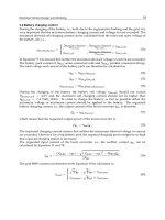
First, acceleration and speed reversal at no load is performed. A speed command of 150
rad/s at 0.5 s is given to the drive system which was initially at rest, and then the speed is
reversed at 3 s. The response of the drive is shown in Fig. 14. Fig. 14 (a) shows reference
(
*

ω
), actual (
ω
), estimated (
ˆ
ω
) speed, and speed estimation error (
ˆ
ω
ω
−
). The module of
the actual (
r
||Ψ ), estimated (
r
ˆ
||
Ψ
) rotor flux, and rotor flux estimation error (
rr
ˆ
||||−
ΨΨ
)
are shown in Fig. 14 (b). Fig. 14 (c) and (d) shows respectively the locus of the actual and
estimated rotor fluxes.
The drive is then run at various speeds under no load condition. It is accelerated from rest to
10 rad/s at 0.5 s, then accelerated further to 50 rad/s, 100 rad/s and 150 rad/s at 1.5 s, 3 s
and 4.5 s respectively. Fig. 15 shows the estimation of rotor flux and speed, and the response

of the sensorless drive system.
Then, the drive is subjected to a slow change in reference speed profile (trapezoidal), the
results of which are shown in Fig. 16.



Fig. 13. Sensorless vector controlled induction motor drive

Further, the performance of the estimator is verified under loaded conditions at various
operating speeds. The fully loaded drive is accelerated to 150 rad/s at 0.5 s and then
decelerated in steps to 100 rad/s, 50 rad/s and 10 rad/s at 1.5 s, 3 s and 4.5 s respectively.
Fig. 17 shows the estimation results and response of the loaded drive system.
Then, we test the performance of the estimator on loading and unloading. The drive at rest
is accelerated at no-load to 150 rad/s at 0.5 s and full load is applied at 1 s; we then remove
the load completely at 2 s. Later, after speed reversal, full load is applied at 4 s, then, the
load is removed completely at 5 s. Fig. 18 shows the estimation results and the response of
the sensorless drive.
*
ω

dc
V
+
+
+
INVERTER
−
−
−
−

+
IM
*
s
d
i
*
s
q
i
abc
ˆ
ω

dq
ROTOR FLUX
&
SPEED
ESTIMATOR
abc
dq
s
i
s
v
*
s
q
v
*

s
d
v
*
s
a
v
*
s
b
v
*
s
c
v
*
ρ
*
r
ψ

FLUX VECTOR
GENERATION
+
ˆ
r
ψ
−
s
d

i
s
q
i
*
s
q
i
*
r
Ψ
s
i
Sensorless Vector Control of Induction Motor Drive - A Model Based Approach

91
0 1 2 3 4 5 6
-200
0
200
Speed [ rad/s ]
Time [ s ]
0 1 2 3 4 5 6
-10
0
10
Time [ s ]
( a )
Speed estim ation error
[ rad/s ]

0 1 2 3 4 5 6
0
0.2
0.4
Time [ s ]
Flux [ Wb ]
0 1 2 3 4 5 6
-0.2
0
0.2
Time [ s ]
( b )
Flux estimation error
[ W b ]
-0.4 -0.3 -0.2 -0.1 0 0.1 0.2 0.3 0.4
-0.4
-0.2
0
0.2
Actual
ψ
r
α
[ Wb ]
( c )
Actual
ψ
r
β
[ W b ]

-0.4 -0.3 -0.2 -0.1 0 0.1 0.2 0.3 0.4
-0.4
-0.2
0
0.2
Estimated
ψ
r
α
[ Wb ]
( d )
Estim ated
ψ
r
β
[ W b ]
Reference speed
Actual speed
Estimated speed
Actual flux
Estimated flux

Fig. 14. Acceleration and speed reversal of the sensorless drive at no-load


0 1 2 3 4 5 6
0
50
100
150

Time [ s ]
Speed [ rad/s ]
0 1 2 3 4 5 6
-10
0
10
Time [ s ]
( a )
Speed estimation error
[ rad/s ]
0 1 2 3 4 5 6
0
0.2
0
.
4
Time [ s ]
Flux [ Wb ]
0 1 2 3 4 5 6
-0.2
0
0.2
Time [ s ]
( b )
Flux estimation error
[ W b ]
-0.4 -0.3 -0.2 -0.1 0 0.1 0.2 0.3 0.4
-0.4
-0.2
0

0.2
Actual
ψ
r
α
[ Wb ]
( c )
Actual
ψ
r
β
[ W b ]
-0.4 -0.3 -0.2 -0.1 0 0.1 0.2 0.3 0.4
-0.4
-0.2
0
0.2
Estimated
ψ
r
α
[ Wb ]
( d )
Estim ated
ψ
r
β
[ W b ]
Reference speed
Actual speed

Estimated speed Actual flux
Estimated flux


Fig. 15. No-load operation of the sensorless drive with step increase in speeds
Electric Machines and Drives

92

0 1 2 3 4 5 6
-200
0
200
Time [ s ]
Speed [ rad/s ]
0 1 2 3 4 5 6
0
0.2
0.4
Time [ s ]
Flux [ Wb ]
0 1 2 3 4 5 6
-10
0
10
Time [ s ]
(a)
Speed estimation error
[ rad/s ]
0 1 2 3 4 5 6

-0.2
0
0.2
Time [ s ]
(b)
Flux estimation error
[ Wb ]
-0.4 -0.3 -0.2 -0.1 0 0.1 0.2 0.3 0.4
-0.4
-0.2
0
0.2
Actual
ψ
r
α
[ Wb ]
(c)
Actual
ψ
r
β
[ Wb ]
-0.4 0.3 -0.2 -0.1 0 0.1 0.2 0.3 0.4
-0.4
-0.2
0
0.2
Estimated
ψ

r
α
[ Wb ]
(d)
Estimated
ψ
r
β
[ Wb ]
Reference speed
Actual speed
Estimated speed
Actual flux
Estimated flux

Fig. 16. No-load operation of the sensorless drive with trapezoidal reference speed

0 1 2 3 4 5 6
0
100
200
Time [ s ]
Speed [ rad/s ]
0 1 2 3 4 5 6
-10
0
10
Time [ s ]
( a )
Speed estimation error

[ rad/s ]
0 1 2 3 4 5 6
0
0.2
0.4
Time [ s ]
Flux [ W b ]
0 1 2 3 4 5 6
-0.2
0
0.2
Time [ s ]
( b )
Flux estimation error
[ W b ]
-0.4 -0.3 -0.2 -0.1 0 0.1 0.2 0.3 0.4
-0.4
-0.2
0
0.2
Actual
ψ
r
α
[ Wb ]
( c )
Actual
ψ
r
β

[ W b ]
-0.4 -0.3 -0.2 -0.1 0 0.1 0.2 0.3 0.4
-0.4
-0.2
0
0.2
Estimatedl
ψ
r
α
[ Wb ]
( d )
E stim atedl
ψ
r
β
[ W b ]
Reference speed
Estimated speed
Actual speed
Actual flux
Estimated flux

Fig. 17. Operation of the sensorless drive at full load at various speeds
Sensorless Vector Control of Induction Motor Drive - A Model Based Approach

93
0 1 2 3 4 5 6
-200
0

200
Time [ s ]
Speed [ rad/s ]
0 1 2 3 4 5 6
0
0.2
0.4
Time [ s ]
Flux [ Wb ]
0 1 2 3 4 5 6
-10
0
10
Time [ s ]
( a )
Speed estimation error
[ rad/s ]
0 1 2 3 4 5 6
-0.2
0
0.2
Time [ s ]
( b )
Flux estimation error
[ Wb ]
-0.4 -0.3 -0.2 -0.1 0 0.1 0.2 0.3 0.4
-0.4
-0.2
0
0.2

Actual
ψ
r
α
[ Wb ]
( c )
Actual
ψ
r
β
[ Wb ]
-0.4 -0.3 -0.2 -0.1 0 0.1 0.2 0.3 0.4
-0.4
-0.2
0
0.2
Estimated
ψ
r
α
[ Wb ]
( d )
Estimated
ψ
r
β
[ Wb ]
Reference speed
Actual speed
Estimated speed

Actual flux
Estimated flux

Fig. 18. Drive response on application and removal of load
4. Conclusion and future works
In this chapter we have presented some methods of sensorless vector control of induction
motor drive using machine model-based estimation. Sensorless vector control is an active
research area and the treatment of the whole model based sensorless vector control will
demand a book by itself.
First, a speed estimation algorithm in vector controlled induction motor drive has been
presented. The proposed method is based on observing a newly defined quantity which is a
function of rotor flux and speed. The algorithm uses command flux for speed computation.
The problem of decrease in estimation accuracy with the decrease in speed was overcome
using a flux observer based on voltage model of the machine along with the observer of the
newly defined quantity, and satisfactory results were obtained.
Then, a joint rotor flux and speed estimation algorithm has been presented. The proposed
method is based on a modified Blaschke equation and on observing the newly defined
quantity mentioned above. Good estimation accuracy was obtained and the response of the
sensorless vector controlled drive was found to be satisfactory.
The mathematical model of the motor used for implementing the estimation algorithm was
derived with the assumption that the rotor speed dynamics is much slower than that of
electrical states. Therefore, increase in estimation accuracy of the proposed algorithms will
be observed with the increase in the size of the machine used.
The machine model developed in this chapter may be used in future for machine parameter
estimation. The newly defined quantity presented in this chapter contains rotor resistance
information as well, in addition to that of rotor flux and speed. Therefore, future research
efforts may be made towards developing rotor resistance estimation algorithm using the
Electric Machines and Drives

94

new machine model. Further, in the proposed algorithms rotor flux was necessary for speed
estimation. Future research efforts may also be made towards developing a speed
estimation algorithm for which the knowledge of rotor flux is not necessary.
5. References
Abbondante, A. & Brennen, M. B. (1975). Variable speed induction motor drives use
electronic slip calculator based on motor voltages and currents. IEEE Trans. Ind.
Appl, Vol. 1A-11, No. 5, Sept/Oct, pp. 483-488.
Ben-Brahim, L. & Kudor, T. (1995). Implementation of an induction motor speed estimator
using neural networks. Proceedings of International Power Electronics Conference, IPEC
1995, Yokohama, April, pp. 52-58.
Bodson, M.; Chiasson, J. & Novotnak, R. T. (1995). Nonlinear Speed Observer for High
Performance Induction Motor Control. IEEE Trans. Ind. Elec, Vol. 42, No. 4, Aug.
pp. 337-343.
Choy, I.; Kwon, S. H.; Lim J. & Hong, S. W. (1996). Robust Speed Estimation for Tacholess
Induction Motor Drives. IEEE Electronics Letters, Vol. 32, No. 19, pp. 1836-1838.
Comnac V.; Cernat M.; Cotorogea, M. & Draghici, I. (2001). Sensorless Direct Torque and
Stator Flux Control of Induction Machines Using an Extended Kalman Filter",
Proceedings of IEEE Int. Conf. on Control Appl, Mexico, Sept. 5-7, pp. 674-679.
Du T.; Vas, P. & Stronach, F. (1995). Design and Application of Extended Observers for Joint
State and Parameter Estimation in High Performance AC Drives. IEE Proc. Elec.
Power Appl., Vol. 142, No. 2, pp. 71-78.
Fodor, D. ; Ionescu, F. ; Floricau, D. ; Six, J.P. ; Delarue, P. ; Diana, D. & Griva, G. (1995).
Neural Networks Applied for Induction Motor Speed Sensorless Estimation.
Proceedings of the IEEE International Symposium on Industrial Electronics, ISIE’ 95, July
10-14, Athens, pp. 181-186.
Gopinath, B. (1971). On the Control of Linear Multiple Input-Output Systems. Bell System
Technical Journal, Vol. 50, No. 3, March, pp. 1063-1081.
Haghgoeian, F.; Ouhrouche, M. & Thongam, J. S. (2005). MRAS-based speed estimation for
an induction motor sensorless drive using neural networks. WSEAS Transactions on
Systems, Vol. 4, No. 12, December, pp. 2346-2352.

Jansen, P. L. & Lorenz, R. D. (1994). A physically insightful approach to the design and
accuracy assessment of flux observers for field oriented induction machine drives.
IEEE Trans. Ind. App., Vol. 30, No. l, Jan. /Feb., pp. 101-110.
Kim, S. H.; Park, T. S.; Yoo, J. Y. & Park, G. T. (2001). Speed-sensorless vector control of an
induction motor using neural network speed estimation. IEEE Trans. Ind. Elec, Vol.
48, No. 3, June, pp. 609-614.
Kim, Y. R.; Sul S. K. & and Park, M. H. (1994). Speed sensorless vector control of induction
motor using extended Kalman filter. IEEE Trans. Ind. Appl., Vol. 30, No. 5,
Sept/Oct, pp. 1225-1233.
Kubota, H.; Matsuse K. & Nakano, T. (1993). DSP-based speed adaptative flux observer of
induction motor. IEEE Trans. Ind. Appl, Vol. 29, No. 2, March/April, pp. 344-348.
Liu, J. J.; Kung, I. C. & Chao, H. C. (2001). Speed estimation of induction motor using a non-
linear identification technique. Proc. Natl. Sci. Counc. ROC (A), Vol. 25, No. 2, pp.
107-114.
Sensorless Vector Control of Induction Motor Drive - A Model Based Approach

95
Ma, X. & Gui, Y. (2002). Extended Kalman filter for speed sensor-less DTC based on DSP.
Proc. of the 4
th
World Cong. on Intelligent Control and Automation, Shanghai, China,
June 10-14, pp. 119-122.
Minami, K.; Veley-Reyez, M.; Elten, D.; Verghese, G. C. & Filbert, D. (1991). Multi-stage
speed and parameter estimation for induction machines. Proceedings of the IEEE
Power Electronics Specialists Conf., Boston, USA, pp. 596-604.
Ohtani, T.; Takada, N. & and Tanaka, K. (1992). Vector control of induction motor without
shaft encoder. IEEE Trans. Ind. Appl, Vol. 28, No. 1, Jan/Feb, pp. 157-164.
Pappano, V.; Lyshevski, S. E. & Friedland, B. (1998). Identification of induction motor
parameters. Proceedings of the 37th IEEE Conf. on Decision and Control, Tampa,
Florida, USA, December 16-18, pp. 989-994.

Peng, F. Z. & Fukao, T. (1994). Robust speed identification for speed sensorless vector
control of induction motors. IEEE Trans. Ind. Appl, Vol. 30, No. 5, Sept/Oct., pp.
1234-1240.
Rowan, T. M. & Kerkman, R. J. (1986). A new synchronous current regulator and an analysis
of current-regulated PWM inverters. IEEE Trans. Ind. Appl, Vol. IA-22, No. 4,
July/Aug., pp. 678-690.
Schauder, C. (1992). Adaptive speed identification for vector control of induction motors
without rotational transducers. IEEE Trans. Ind. Appl, Vol. 28, No. 5, Sept./Oct., pp.
1054-1061.
Sathiakumar, S. (2000). Dynamic flux observer for induction motor speed control.
Proceedings of Australian Universities Power Engineering Conf. AUPEC 2000, Brisbane,
Australia, 24-27 Sept., pp. 108-113.
Simoes, M. G. & Bose, B. K. (1995). Neural network based estimation of feedback signals for
a vector controlled induction motor drive. IEEE Trans. Ind. Appl., Vol. 31,
May/June, pp. 620-629.
Tajima, H. & Hori, Y. (1993). Speed sensorless field-orientation control of the induction
machine. IEEE Trans. Ind. Appl., Vol. 29, No. 1, pp. 175-180.
Thongam, J. S. & Thoudam, V. P. S. (2004). Stator flux based speed estimation of induction
motor drive using EKF. IETE Journal of Research, India, Vol. 50, No. 3. May-June, pp
191-197.
Thongam, J. S. & Ouhrouche, M. (2006). Flux estimation for speed sensorless rotor flux
oriented controlled induction motor drive. WSEAS Transactions on Systems, Vol. 5,
No. 1, Jan., pp. 63-69.
Thongam, J. S. & Ouhrouche, M. (2007). A novel speed estimation algorithm in indirect
vector controlled induction motor drive. International Journal of Power and Energy
Systems, Vol. 27, No. 3, 2007, pp. 294-298.
Toqeer, R. S. & Bayindir, N. S. (2003). Speed estimation of an induction motor using Elman
neural network. Neuro Computing, Volume 55, Issues 3-4, October, pp. 727- 730.
Velez-Reyes, M.; Minami, K. & Verghese, G. C. (1989). Recursive speed and parameter
estimation for induction machines", IEEE/IAS Ann. Meet. Conf. Rec., San Diego, pp.

607-611.
Veleyez-Reyes, M. & Verghese, G. C. (1992). Decomposed algorithms for speed and
parameter estimation in induction machines. IFAC Symposium on Nonlinear Control
System Design, Bordeaux, France, pp. 77-82.
Electric Machines and Drives

96
Verghese, G. C. & Sanders, S. R. (1988). Observers for flux estimation in induction machines.
IEEE Trans. Ind. Elec, Vol. 35, No. 1, Feb., pp. 85-94.
Yan, Z.; Jin C. & Utkin, V. I. (2000). Sensorless sliding-mode control of induction motors.
IEEE Trans. Ind. Elec, Vol. 47, No. 6, Dec., pp. 1286-1297.

Feedback Linearization of Speed-Sensorless
Induction Motor Control with Torque
Compensation
1. Introduction
This chapter addresses the problem of controlling a three-phase Induction Motor (IM) without
mechanical sensor (i.e. speed, position or torque measurements). The elimination of the
mechanical sensor is an important advent in the field of low and medium IM servomechanism;
such as belt conveyors, cranes, electric vehicles, pumps, fans, etc. The absence of this sensor
(speed, position or torque) reduces cost and size, and increases reliability of the overall
system. Furthermore, these sensors are often difficult to install i n certain applications a nd
are susceptible to electromagnetic interference. In fact, sensorless servomechanism may
substitute a measure value by an estimated one without deteriorating the drive dynamic
performance especially under uncertain load torque.
Many approaches for IM sensorless servomechanism have been proposed in the literature
is related to vector-controlled methodologies. One of the proposed nonlinear control
methodologies is based on Feedback Linearization Control (FLC), as first introduced by
(Marino et al., 1990). F LC provides rotor speed regulation, rotor flux amplitude decoupling
and torque compensation. Although the strategy presented by (Marino et al., 1990) was not

a sensorless control strategy, fundamental principles of FLC follow servomechanism design
of sensorless control strategies, such as (Gastaldini & Grundling, 2009; M arino et al., 2004;
Montanari et al., 2007; 2006).
The purpose of this chapter is to present the development of two FLC control strategies in the
presence of torque disturbance or load variation, especially under low rotor speed conditions.
Both control strategies are easily implemented in fixed point DSP, such as TMS320F2812 used
on real time experiments and can be easily reproduced in the industry. Furthermore, an
analysis comparing the implementation and the limitation of both strategies is presented. In
order to implement the control law, these algorithms made use of only two-phase IM stator
currents measurement. The values of rotor speed and load torque states used in the control
algorithm are estimated using a Model Reference Adaptive System (MRAS) (Peng & Fukao,
1994) and a Kalman filter (Cardoso & Gründling, 2009), respectively.
This chapter is organized as follows: Section 2 presents the fi fth-order IM mathematical
model. Section 3 introduces the feedback linearization modelling of IM control. A simplified
Cristiane Cauduro Gastaldini
1
, Rodrigo Zelir Azzolin
2
,
Rodrigo Padilha Vieira
3
and Hilton Abílio Gründling
4
1,2,3,4
Federal University of Santa Maria
2
Federal University of Rio Grande
3
Federal University of Pampa
Brazil

6
FLC control strategy is described in Section 4. The proposed methods for speed and torque
estimation, M RAS and Kalman filter algorithms, respectively, are developed in Sections 5 and
6. State variable filter is used to obtain derivative signals necessary for implementation of the
control algorithm, and this is presented in section 7. Digital implementation in fixed point
DSP TMS320F2812 and real time experimental results are given in Section 8. Finally, Section 9
presents the conclusions.
2. Induction motor mathematical model
A three-phase N pole pair induction motor is expressed in an equivalent two-phase model in
an arbitrary rotating reference frame (q-d), according to (Krause, 1986) and (Leonhard, 1996)
according to the fifth-order model, as
d
dt
I
qs
= −a
12
I
qs
−ω
s
I
ds
+ a
13
a
11
λ
qr
− a

13
Nωλ
dr
+ a
14
V
qs
(1)
d
dt
I
ds
= −a
12
I
ds
+ ω
s
I
qs
+ a
13
a
11
λ
dr
+ a
13
Nωλ
qr

+ a
14
V
ds
(2)
d
dt
λ
qr
= −a
11
λ
qr
−
(
ω
s
− Nω
)
λ
dr
+ a
11
L
m
I
qs
(3)
d
dt

λ
dr
= −a
11
λ
dr
+
(
ω
s
− Nω
)
λ
qr
+ a
11
L
m
I
ds
(4)
d
dt
ω
= μ ·

λ
dr
I
qs

−λ
qr
I
ds

−
B
J
ω
−
T
L
J
(5)
T
e
= μ · J ·

λ
dr
I
qs
−λ
qr
I
ds

(6)
In equations (1)-(6): I
s

=

I
qs
, I
ds

, λ
r
=

λ
qr
, λ
dr

and V
s
=

V
qs
, V
ds

denote stator current,
rotor flux and stator voltage vectors, where subscripts d and q stand for vector components in
(q-d) reference frame; ω is the rotor speed, the load torque T
L
,electrictorqueT

e
and ω
s
is the
stationary speed, θ
0
is the angular position of the (q-d) reference frame with respect to a fixed
stator reference frame (α-β) , where physical variables are defined. Transformed variables
related to three-phase (RST) system are given by
x
αβ
= K · x
RST
(7)
Let
x
qd
= e
jθ
0
x
αβ
(8)
with e
jθ
0
=

cos θ
0

−sin θ
0
sin θ
0
cos θ
0

and K
=

2
3
⎡
⎢
⎣
1
−
1
2
−
1
2
0
−
√
3
2
−
√
3

2
⎤
⎥
⎦
.
x
qd
and x
αβ
stand for two-dimensional voltage flux and stator current vector, respectively on
(q-d) and ( α-β)reference frame.
The relations between mechanical and electrical parameters in the above e quations are
a
0
Δ
= L
s
L
r
− L
2
m
, a
11
Δ
=
R
r
L
r

, a
12
Δ
=

L
s
L
r
a
0
R
s
L
s
+
L
2
m
a
0
a
11

, a
13
Δ
=
L
m

a
0
, a
14
Δ
=
L
r
a
0
and μ
Δ
=
NL
m
JL
r
;
98
Electric Machines and Drives
where R
s
, R
r
, L
s
and L
r
are the stator/rotor resistances and inductances, L
m

is the magnetizing
inductance, J is the rotor inertia, B is the viscous coefficient and N is the number of pole pairs.
In the control design, the viscous coefficient of (5) is considered to be approximately zero, i.e.
B
≈ 0.
3. Feedback Linearization Control
The feedback Linearization Control (FLC) general specifications are two outputs - rotor speed
and rotor flux modulus, as
y
1
=

ω

λ
2
qr
+ λ
2
dr

T
Δ
=

ω
|
λ
r
|


T
(9)
which is controlled b y two-dimensional stator voltage vector V
s
, on the basis of measured
variables ve ctor y
2
= I
s
. The development concept of this control strategy is completely
described in (Marino et al., 1990) and it will be omitted here. Following the concept of indirect
field orientation developed by Blaschke, (Krause, 1986) and (Leonhard, 1996), the purpose of
FLC control is to align rotor flux vector with the d-axis reference frame, i.e.
λ
dr
=
|
λ
r
|
λ
qr
= 0 (10)
The condition expressed in (10) guarantees the exact decoupling of flux dynamics of (1)-(4)
from the speed dynamics. Once rotor flux is not directly measured, only asymptotic field
orientation is possible, according to (Marino et al., 1990) and (Peresada & Tonielli, 2000), then
lim
t→∞
λ

dr
=
|
λ
r
|
lim
t→∞
λ
qr
= 0 (11)
It is defined y
∗
1
=

ω
re f
λ
∗
r

T
,whereω
re f
and λ
∗
r
are reference trajectories of rotor speed
and rotor flux. The speed tracking, flux regulation control problem under speed sensorless

conditions is formulated considering IM model (1)-(5) under the following conditions:
(a) Stator currents are measurable;
(b) Motor parameters are known and considered constant;
(c) Load torque is estimated and it is applied after motor flux excitation;
(d) Initial conditions of IM state variables are known;
(e) λ
∗
r
is the flux constant reference value and estimated speed

ω and reference speed ω
re f
are
the smooth reference bounded speed signals.
FLC equations are developed considering the fifth-order IM model under the assumption that
estimated speed tracks real speed, and therefore it is acceptable to replace measured speed
with estimated speed ( i.e.

ω
k
≈ ω). In addition, the torque value is estimated using a Kalman
filter. Fig. 1 presents the block diagram of FLC Control.
3.1 Flux controller
From the decoupling properties of field oriented transformation (10), the control objective of
the flux controller is to generate a flux vector aligned with the d-axis to guarantee induction
motor magnetization.
Then, substituting (10) in (4)
i
∗
ds

=

a
11
λ
∗
r
+
d
dt
|
λ
r
|

1
a
11
L
m
(12)
99
Feedback Linearization of Speed-Sensorless Induction Motor Control with Torque Compensation
Speed MRAS
Estimation
µ
ω
rst
I
RST

V
RST
Indution
3 Motorf
Kalman
Filter
µ
k
ω
Ktn
1/J
s + B/J
ò
µ
ω
k
PI
-
+
Flux
Control
Current
Control I
ds
PI
ds
u
ds
u
-

+
Speed
Control
-
+
Current
Control I
qs
qs
u
qs
u
q
i
qs
v
*
ds
v
*
ds
i
*
qs
i
*
qs
d
I
dt

qs
I
ref
d
dt
w
L
T
L
T
ds
v
*
qs
v
*
q
q
-
+
-
+
µ
ω
k
µ
ω
k
Sαβ
v

Sαβ
i
ab
qd
rst
qs
I
ds
I
-
+
w
ds
d
I
dt
SVF
SVF
SVF
ref
w
SVF
r
λ
L
T
m
T
e
T

+
+
ω
s
PI
PI
e
w
-
+
µ
ω
k
ω
ref
PI
PI
q
i
d
dt
r
λ
Fig. 1. Feedback Linearization Control proposed
The rotor flux
|
λ
r
|
is estimated b y a model derived from the induction motor mathematical

model, (3) and (4), that makes use of measured stator currents

I
qs
, I
ds

and estimated speed

ω variables.
d
dt
λ
r
= −a
11
λ
r
− j
(
ω
s
− Nω
)
λ
r
+ a
11
L
m

I
s
(13)
where the stationary speed is ω
s
= N

ω +
a
11
L
m
λ
∗
i
∗
qs
. The digital implementation of the flux
controller is made using Euler discretization and the derivative rotor flux signal is obtained
by a state variable filter (SVF).
3.2 Speed controller
The speed control algorithm uses the same strategy adopted for the flux subsystem and it is
computed from (5), as
i
q
=
1
μλ
∗
r



T
L
J
+
d
dt
ω
re f

(14)
To compensate for speed error between estimated speed and reference speed, (i.e.
e
ω
=

ω
−ω
re f
), a proportional integral compensation is proposed, as follows
100
Electric Machines and Drives
i
q
=

k
p_iq
+

k
i_iq
s

e
ω
(15)
These gains values
(k
p_iq
, k
i_iq
) are determined considering an induction motor mechanical
model. The reference quadrature component stator speed current is derived from (14)-(15), as
i
∗
qs
= i
q
−i
q
(16)
In DSP implementation, the speed controller is discretized using the Euler method and the
rotor speed derivative (14) is computed by a SVF.
3.3 Currents controller
From (1) and (2), the currents controller is obtained, as
u
qs
=
1

a
14

a
12
i
∗
qs
+ ω
s
i
∗
ds
+ a
13
λ
∗
r
N

ω
re f
+ e
ω

+
d
dt
I
qs


(17)
and
u
ds
=
1
a
14

a
12
i
∗
ds
+ ω
s
i
∗
qs
+ a
11
a
13
λ
r
+
d
dt
I

ds

(18)
where proportional integral gains of the current error
u
qs
=

k
pv
+
k
iv
s


i
qs
(19)
and
u
ds
=

k
pv
+
k
iv
s



i
ds
(20)
in which

i
qs
= I
qs
−i
∗
qs
and

i
ds
= I
ds
−i
∗
ds
.
These gains
(k
pv
, k
iv
) are determined considering a simplified induction motor electrical

model, which is obtained by load and locked rotor test. Hence, current controllers are
expressed as
v
∗
qs
= u
qs
−u
qs
(21)
v
∗
ds
= u
ds
−u
ds
(22)
In DSP, currents controller are digitally implemented using discretized equation (17)-(22)
based on the Euler method, and the stator current derivative is obtained by SVF using stator
currents measures.
4. Simplified feedback linearization control
In order to reduce the number of computation requirements, a simplified feedback
linearization control scheme is proposed. In this control scheme, one part of the current
controller (6)-(7) is suppressed and only a proportional integral controller is used. This
modification minimizes the influence of parameters variation in the control system.
Fig. 2 presents the block diagram of the Simplified FLC proposed.
The currents controller of simplified FLC are defined as
101
Feedback Linearization of Speed-Sensorless Induction Motor Control with Torque Compensation

v
∗
qs
=

k
pv
+
k
iv
s


i
qs
(23)
v
∗
ds
=

k
pv
+
k
iv
s


i

ds
(24)
Ktn
1/J
s + B/J
ò
µ
ω
k
PI
Flux
Control
PI
-
+
Speed
Control
e
w
q
i
q
i
ds
v
*
ds
i
*
ref

d
dt
w
L
T
q
-
+
-
+
µ
ω
k
ω
ref
qs
I
ds
I
-
+
SVF
ref
w
SVF
r
λ
L
T
m

T
e
T
+
+
ω
s
PI
PI
qs
v
*
qs
i
*
qs
I
-
+
PI
PI
d
dt
r
λ
Speed MRAS
Estimation
µ
ω
rst

I
RST
V
RST
Indution
3 Motorf
Kalman
Filter
µ
k
ω
L
T
ds
v
*
qs
v
*
q
Sαβ
v
Sαβ
i
ab
qd
rst
w
Fig. 2. Proposed Simplified Feedback Linearization Control
Flux and Speed Controller are computed exactly as in the previous scheme, as ( 12) and

(14)-(16).
5. Speed estimation - MRAS algorithm
A squirrel-cage three-phase induction motor model expressed in a stationary frame can be
modelled using complex stator and rotor voltage a s in (Peng & Fukao, 1994)
v
s
= R
s
i
s
+ L
s
d
dt
i
s
+ L
m
d
dt
i
r
(25)
for squirrel-cage IM v
r
= 0
0
= R
r
i

r
− jNωL
r
i
r
− jNωL
m
i
s
+ L
r
d
dt
i
r
+ L
m
d
dt
i
s
(26)
102
Electric Machines and Drives
The voltage and the current space vectors are given as x = x
α
+ jx
β
, x ∈
{

v
s
, i
s
, i
r
}
, relative
to the transformed variables p resent in (7). The induction motor magnetizing current is
expressed by
i
m
=
L
r
L
m
i
r
+ i
s
(27)
Two independent observers are derived to estimate the components of the
counter-electromotive vectors.
e
m
=
L
2
m

L
r
i
m
=
L
2
m
L
r

ωi
m
−
1
T
r
i
m
+
1
T
r
i
s

(28)
e
m
= v

s
− R
s
i
s
−σL
s
d
dt
i
s
(29)
where σ
= 1 −
L
m
L
s
L
r
. The instantaneous reactive power maintains the magnetizing current,
and its value is defined by cross product of the counter-electromotive and stator current vector
q
m
= i
s
⊗e
m
(30)
Substituting (28) and (29) for e

m
in (30) and noting that i
s
⊗i
s
= 0, which gives
q
m
= i
s
⊗

v
s
−σL
s
d
dt
i
s

(31)
and
q
m
=
L
2
m
L

r

(
i
m
i
s
)
ω +
1
T
r
(
i
m
⊗i
s
)

(32)
Then, q
m
is the reference model of reactive power and q
m
is the adjustable model. The
estimated speed is produced by the proportional integral adaptation mechanism error of both
models, and an MRAS system can be drawn as in Fig.3
This algorithm is customary for speed estimation and simple to implement in fixed point DSP,
such as i n (Gastaldini & G rundling, 2009; Orlowska-Kowalska & Dybkowski, 2010; Vieira
et al., 2009).

The SVF blocks are state variable filters and are explained in greater detail in Section 7. These
filters compute derivative signals and are applied in voltage signals to avoid addition noise
and phase delay among the vectors as was proposed by (Martins et al., 2006).
6. Load torque estimation - Kalman filter
The reduced mechanical IM system can be represented by the following equations
d
dt

ω
T
L

=
⎡
⎣
−
B
n
J
−
1
J
00
⎤
⎦

ω
T
L


+
⎡
⎣
1
J
0
⎤
⎦
T
e
(33)
y
=

10


ω
T
L

(34)
The Kalman Filter could be used to provide the value of torque load or disturbances - T
L
.
Since (15)-(16) is nonlinear, the Kal man filter linearizes the model at the actual operating
103
Feedback Linearization of Speed-Sensorless Induction Motor Control with Torque Compensation
-
+

$$
=Ä
m
Sαβ
m
qi e
µ
k
RR
d11
dt T T
=w Ä - +
mmmSαβ
iiii
$µ
k
m
RR
11
L
TT
æö
=wÄ- +
ç÷
èø
m
m m Sαβ
eiii
PI
Kalman Filter

m
qD
Adaptative Model
µ
k
w
=Ä
mSαβ m
qi e
Reference Model
ss
d
RL
dt
æö
=- +s
ç÷
èø
m Sαβ Sαβ Sαβ
ev i i
Sαβ
v
Sαβ
i
µ
w
m
q
$
m

q
SVF
SVF
‘
Fig. 3. Reactive Power MRAS Speed Estimation
point ( Aström & Wittenmark, 1997). In addition, this filter takes into account the signal
noise, which could be generated as pulse width modulation drivers. Assuming the definitions
x
k
=


ω
k

T
L

T
, A
m
=
⎡
⎣
−
B
n
J
−
1

J
00
⎤
⎦
, B
m
=
⎡
⎣
1
J
0
⎤
⎦
, C
m
=

10

and y
k
=

ω.
Then, the recursive equation for the discrete time Kalman Filter (De Campos et al., 2000) is
described by
K
(k)=P (k)C
T

m

C
m
P(k)C
T
m
+ R

−1
(35)
where K
(k) is the Kalman gain. The covariance matrix P(k) is given by
P
(k + 1)=
(
I −A
m
t
s
)(
P(k) − K(k )C
m
P(k)
)(
I −A
m
t
s
)

T
+
(
B
m
t
s
)
Q
(
B
m
t
s
)
T
(36)
Therefore, the estimated torque

T
L
is one observed state of the Kalman filter
x
k
(k + 1)=
(
I −A
m
t
s

)
x
k
(k)+B
m
t
s
u(k)+
(
I − A
m
t
s
)
K(k)
(

ω
−C
m
x
k
(k)
)
(37)
giving

ω
≈


ω
k
and x
k
(k)=


ω
k
T
L

T
.
The matrices R and Q are defined according to noise elements of predicted state variables,
taking into account the measurement noise covariance R and the plant noise covariance Q.
7. State variable filter
The state variable filter (SVF) is used to mathematically evaluate differentiation signals. This
filter is necessary in the implementation of FLC and MRAS algorithms. The transfer function
of SVF is of second order as it is necessary to obtain the first order derivative.
G
sv f
=
ω
sv f

s
+ ω
sv f


2
(38)
104
Electric Machines and Drives
where ω
sv f
is the filter bandwidth defined at around 5 to 10 times the input frequency signal
u
sv f
.
The discretized transfer function, using the Euler method, can be performed in state-space as
x
svf
(
k + 1
)
=
A
svf
x
svf
(
k
)
+
B
svf
u
sv f
(

k
)
(39)
where A
svf
=

11
−ω
2
sv f
1 −2ω
sv f

, B
svf
=

0
ω
2
svf

and x
svf
=

x
1
x

2

.
The state variables x
1
and x
2
represent the input filtered signal and input derivative signal.
8. Experimental results
Sensorless control schemes were implemented in DSP based platform using TMS 320F2812.
Experimental results were carried out on a motor with specifications: 1.5cv, 380V, 2.56A, 60
Hz, R
s
= 3.24Ω, R
r
= 4.96Ω, L
r
= 404.8mH, L
s
= 402.4mH, L
m
= 388.5mH, N = 2and
nominal speed of 188 rad/s.
The experimental analyses are carried out with the following operational sequence:
1) The motor is excited (during 10 s to 12 s) using a smooth flux reference trajectory.
2) Starting from zero initial value, the rotor speed reference grows linearly until it reaches the
reference value. Thus, the reference rotor speed value is kept constant.
3) During stand-state, a step constant load torque is applied.
In order to generate load variation for torque disturbance analyses, the DC motor is connected
to an induction motor driving-shaft. Then, the load shaft varies in accordance with DC motor

field voltage and inserting a resistance on its armature. Fig. 4 and Fig. 5 depict performance
of both control schemes: FLC control and simplified FLC control with rotor speed reference of
18 rad/s. In these figures measure speed, estimated speed, stator (q-d) currents and estimated
torque are illustrated.
Fig.6 and Fig. 7 present experimental results with 36 rad/s rotor speed reference.
Fig. 8 and Fig. 9 show FLC control and Simplified FLC with 45 rad/s rotor speed reference.
The above figures present experimental results for low rotor speed range of FLC control and
Simplified FLC control applying load torque. In accordance with the figures above, both
control schemes present similar performances in steady state. It is verified that both schemes
respond to compensated torque variations. W ith respect to Simplified FLC, it is necessary to
carrefully select fixed gains in order to guarantee the alignment of the rotor flux on the d axis.
9. Conclusion
Two different sensorless IM control schemes were proposed and developed based on
nonlinear control - FLC Control and Simplified FLC Control. These control schemes are
composed of a flux-speed controller, which is derived from a fifth-order IM model. In the
implementation of feedback linearization control (FLC), the control algorithm presents a large
number of computational requirements. In the simplified FLC scheme, a substitution of FLC
currents c ontrollers by two PI controllers is proposed to generate the stator drive voltage.
In order to provide the rotor speed for both control schemes, a MRAS algorithm based on
reactive power is applied.
To correctly evaluate whe ther this Si mplified FLC does not affect co ntrol performance, a
comparative experimental analysis of a FLC control and a simplified FLC control is presented.
Experimental results in DSP TMS 320F2812 platform show the performance of both systems
105
Feedback Linearization of Speed-Sensorless Induction Motor Control with Torque Compensation
0 10 20 30 40 50 60 70
0
0.5
1
1.5

2
Current I
d
(A)
Time(s)
(a) IM Stator Current I
ds
0 10 20 30 40 50 60 70
−0.5
0
0.5
1
1.5
2
Current I
q
(A)
Time(s)
(b) IM Stator Current I
qs
0 10 20 30 40 50 60 70
−5
0
5
10
15
20
Rotor Speed (rad/s)
Time(s)

ω
ˆω
k
(c) Rotor Speed - Estimated and Encoder Measurement
0 10 20 30 40 50 60 70
−2
−1
0
1
2
Load Torque (N.m)
Time(s)
(d) Estimated Load Torque
Fig. 4. FLC control with 18 rad/s rotor speed reference
106
Electric Machines and Drives
0 10 20 30 40 50 60 70
0
0.5
1
1.5
2
Current I
d
(A)
Time(s)
(a) IM Stator Current I
ds
0 10 20 30 40 50 60 70

−0.5
0
0.5
1
1.5
Current I
q
(A)
Time
(
s
)
(b) IM Stator Current I
qs
0 10 20 30 40 50 60 70
−5
0
5
10
15
20
Rotor Speed (rad/s)
Time(s)


ω
ˆω
k
(c) Rotor Speed - Estimated and Encoder Measurement
0 10 20 30 40 50 60 70

−0.5
0
0.5
1
1.5
Load Torque (N.m)
Time(s)
(d) Estimated Load Torque
Fig. 5. Simplified FLC control with 18 rad/s rotor speed reference
107
Feedback Linearization of Speed-Sensorless Induction Motor Control with Torque Compensation
0 10 20 30 40 50 60 70
−0.5
0
0.5
1
1.5
Current I
d
(A)
Time(s)
(a) IM Stator Current I
ds
0 10 20 30 40 50 60 70
−0.5
0
0.5
1
1.5
2

Current I
q
(A)
Time(s)
(b) IM Stator Current I
qs
0 10 20 30 40 50 60 70
0
10
20
30
40
Rotor Speed (rad/s)
Time(s)


ω
ˆω
k
(c) Rotor Speed - Estimated and Encoder Measurement
0 10 20 30 40 50 60 70
−2
−1
0
1
2
Load Torque (N.m)
Time(s)
(d) Estimated Load Torque
Fig. 6. FLC control with 36 rad/s rotor speed reference

108
Electric Machines and Drives