Electric Machines and Drives part 7 ppt
Bạn đang xem bản rút gọn của tài liệu. Xem và tải ngay bản đầy đủ của tài liệu tại đây (443.96 KB, 20 trang )
0 10 20 30 40 50 60 70
0
0.5
1
1.5
2
2.5
Current I
d
(A)
Time(s)
(a) IM Stator Current I
ds
0 10 20 30 40 50 60 70
−1
0
1
2
3
Current I
q
(A)
Time(s)
(b) IM Stator Current I
qs
0 10 20 30 40 50 60 70
0
10
20
30
40
Rotor Speed (rad/s)
Time(s)
ω
ˆω
k
(c) Rotor Speed - E stimated and Encoder Measurement
0 10 20 30 40 50 60 70
−1
0
1
2
Load Torque (N.m)
Time(s)
(d) Estimated Load Torque
Fig. 7. Simplified FLC control with 36 rad/s rotor speed reference
109
Feedback Linearization of Speed-Sensorless Induction Motor Control with Torque Compensation
0 10 20 30 40 50 60 70
−1
−0.5
0
0.5
1
1.5
Current I
d
(A)
Time(s)
(a) IM Stator Current I
ds
0 10 20 30 40 50 60 70
−1
0
1
2
3
Current I
q
(A)
Time(s)
(b) IM Stator Current I
qs
0 10 20 30 40 50 60 70
−10
0
10
20
30
40
50
Rotor Speed (rad/s)
Time(s)
ω
ˆω
k
(c) Rotor Speed - E stimated and Encoder Measurement
0 10 20 30 40 50 60 70
−2
−1
0
1
2
Load Torque (N.m)
Time(s)
(d) Estimated Load Torque
Fig. 8. FLC control with 45 rad/s rotor speed reference
110
Electric Machines and Drives
0 10 20 30 40 50 60 70
0
0.5
1
1.5
2
2.5
Current I
d
(A)
Time(s)
(a) IM Stator Current I
ds
0 10 20 30 40 50 60 70
−1
0
1
2
3
Current I
q
(A)
Time(s)
(b) IM Stator Current I
qs
0 10 20 30 40 50 60 70
−10
0
10
20
30
40
50
Rotor Speed (rad/s)
Time(s)
ω
ˆω
k
(c) Rotor Speed - E stimated and Encoder Measurement
0 10 20 30 40 50 60 70
−1
0
1
2
Load Torque (N.m)
Time(s)
(d) Estimated Load Torque
Fig. 9. Simplified FLC control with 45 rad/s rotor speed reference
111
Feedback Linearization of Speed-Sensorless Induction Motor Control with Torque Compensation
in the 18rad/s, 36 rad/s and 45 rad/s rotor speed range. Both control schemes present
similar performance in s teady-state. Hence, the proposed modification of the FLC control
allows a simplification of the control algorithm without deterioration in control performance.
However, it may necessary to carefully evaluate the gain selection in the simplified FLC
control, to guarantee rotor flux alignment on the d axis, as well as, to guarantee speed-flux
decoupling. Both control schemes indicate sensitivity with model parameter variation, and
one way to overcome this would be the is development of an adaptive FLC control laws on
FLC control.
10. References
Aström, K. & Wittenmark, B. (1997). Computer-Controlled Systems: Theory and Design,
Prentice-Hall.
Cardoso, R. & Gründling, H. A. (2009). Grid synchronization and voltage a nalysis based on
the kalman filter, in V. M. Moreno & A. Pigazo (eds), Kalman Filter Recent Advances
and Applications, InTech, Croatia, pp. 439–460.
De Campos, M., Caratti, E. & Grundling, H. (2000). Design of a position servo with induction
motor using self-tuning regulator and kalman filter, Conference Record of the 2000 IEEE
Industry Applications Conference, 2000.
Gastaldini, C. & Grundling, H. (2009). Speed-sensorless induction motor control with torque
compensation, 13th European Conference on Power Electronics and Applications, EPE ’09,
pp. 1 –8.
Krause, P. C. (1986). Analysis of electric machinery, McGraw-Hill.
Leonhard, W. (1996). Control of Electrical Drives,Springer-Verlag.
Marino, R., Peresada, S. & Valigi, P. (1990). Adaptive partial feedback linearization of
induction motors, Proceedings of the 29th IEEE Conference on Decision and Control, 1990,
pp. 3313 –3318 vol.6.
Marino, R., Tomei, P. & Verrelli, C. M. (2004). A global tracking control for speed-sensorless
induction motors, Automatica 40(6): 1071 – 1077.
Martins, O., Camara, H. & Grundling, H. (2006). Comparison between mrls and mras applied
to a speed sensorless induction motor drive, 37th IEEE Power Electronics Specialists
Conference, PESC ’06., pp. 1 –6.
Montanari, M., Peresada, S., Rossi, C. & Tilli, A. (2007). Speed sensorless control of induction
motors based on a reduced-order adaptive observer, IEEE Transactions on Control
Systems Technology 15(6): 1049 –1064.
Montanari, M., Peresada, S. & Tilli, A. (2006). A speed-sensorless indirect field-or iented
control for induction motors based on high gain speed estimation, Automatica
42(10): 1637 – 1650.
Orlowska-Kowalska, T. & Dybkowski, M. (2010). Stator-current-based mras estimator for a
wide range speed-sensorless induction-motor drive, IEEE Transactions on Industrial
Electronics 57(4): 1296 –1308.
Peng, F Z. & Fukao, T. (1994). Robust speed identification for speed-sensorless vector control
of induction motors, IEEE Transactions on Industry Applications 30(5): 1234 –1240.
Peresada, S. & Tonielli, A. (2000). High-performance robust speed-flux tracking controller for
induction motor, International Journal of Adaptive Control and Signal Processing, 2000.
Vieira, R., Azzolin, R. & Grundling, H. (2009). A sensorless single-phase induction motor drive
with a mrac controller, 35th Annual Conference of IEEE Industrial Electronics,IECON
’09., pp. 1003 –1008.
112
Electric Machines and Drives
1. Introduction
DFIG wind turbines are nowadays more widely used especially in large wind farms. The
main reason for their popularity when connected to the electrical network is their ability to
supply power at constant voltage and frequency while the rotor speed varies, which makes
it suitable for applications with variable speed, see for instance (10), (11). Additionally,
when a bidirectional AC-AC converter is used in the rotor circuit, the speed range can be
extended above its synchronous value recovering power in the regenerative operating mode
of the machine. The DFIG concept also provides the possibility to control the overall system
power factor. A DFIG wind turbine utilizes a wound rotor that is supplied from a frequency
converter, providing speed control together with terminal voltage and power factor control
for the overall system.
DFIGs have been traditionally used to convert mechanical power into electrical power
operating near synchronous speed. Some advantages of DFIGs over synchronous or squirrel
cage generators include the high overall efficiency of the system and the low power rating
of the converter, which is only rated by the maximum rotor voltage and current. In a
typical scenario the prime mover is running at constant speed, and the main concern is the
static optimization of the power flow from the primary energy source to the grid. A good
introduction to the operational characteristic of the grid connected DFIG can be found in (5).
We consider in this paper the isolated operation of a DFIG driven by a prime mover, with
its stator connected to a load—which is in this case an IM. Isolated generating units are
economically attractive, hence increasingly popular, in the new era of the deregulated market.
The possibility of a DFIG supplying an isolated load has been indicated in (6), (7) where some
M. Becherif
1
, A. Bensadeq
2
, E. Mendes
3
, A. Henni
4
,
P. Lefley
5
and M.Y Ayad
6
1
UTBM, FEMTO-ST/FCLab, UMR CNRS 6174, 90010 Belfort Cedex
2
AElectrical Power & Power Electronics Group, Department of Engineering
3
Grenoble INP - LCIS/ESISAR, BP 54 26902 Valence Cedex 9
4
Alstom Power - Energy Business Management
5
Electrical Power & Power Electronics Group, Department of Engineering
University of Leicester
6
IEEE Member
1,3,4,6
France
2,5
UK
From Dynamic Modeling to Experimentation of
Induction Motor Powered by Doubly-Fed
Induction Generator by Passivity-Based Control
7
mention is made of the steady–state control problem. In (8) a system is presented in which the
rotor is supplied from a battery via a PWM converter with experimental results from a 200W
prototype. A control system based on regulating the rms voltage of the DFIG is used which
results in large voltage deviations and very slow recovery following load changes. See also
(9; 12) where feedback linearization and sliding mode principles are used for the design of the
motor speed controller.
This paper presents a dynamic model of the DFIG-IM and proves that this system is
Blondel-Park transformable. It is also shown that the zero dynamics is unstable for a certain
operating regime. We implemented the passivity-based controller (PBC) that we proposed
in (3) to a 200W DFIG interconnected with an IM prototype available in IRII-UPC (Institute
of Robotics and Industrial Informatics - University Polytechnic of Catalonia). The setup
is controlled using a computer running RT-Linux. The whole system is decomposed in a
mechanical subsystem which plays the role of the mechanical speed loop, controlled by a
classical PI and an electrical subsystem controlled by the PBC where the model inversion was
used to build a reference model.
The proposed PBC achieves the tracking control of the IM mechanical rotor speed and flux
norm, the practical advantage of the PBC consists of using only the measurements of the two
mechanical coordinates (Motor and Generator positions). The experiments have shown that
the PBC is robust to variations in the machines’ parameters.
In addition to the PBC applied to the electrical subsystem, we proposed a classical PI
controller, where the rotor voltage control law is obtained via a control of the stator currents
toward their desired values, those latter are obtained by the inversion of the model.
In the sequel, and for the control of the electrical subsystem a combination of the PBC +
Proportional action for the control of the stator currents is applied. The last controller is a
combination of PBC + PI action for the control of the stator currents.
The stability analysis is presented. The simulations and practical results show the
effectiveness of the proposed solutions, and robustness tests on account of variations in
the machines’ parameters are also presented to highlight the performance of the different
controllers.
The main disadvantage of the DFIG is the slip rings, which reduce the life time of the
machine and increases the maintenance costs. To overcome this drawback an alternative
machine arrangement is proposed, in section 6, which is the Brushless Doubly Fed twin
Induction Generator (BDFTIG). The system is anticipated as an advanced solution to the
conventional doubly fed induction generator (DFIG) to decrease the maintenance cost and
develop the system reliability of the wind turbine system. The proposed BDFTIG employs two
cascaded induction machines each consisting of two wound rotors, connected in cascade to
eliminate the brushes and copper rings in the DFIG. The dynamic model of BDFTIG with two
machines’ rotors electromechanically coupled in the back-to-back configuration is developed
and implemented using Matlab/Simulink.
2. System configuration and mathematical model
The configuration of the system considered in this paper is depicted in Fig.1. It consists of a
wound rotor DFIG, a squirrel cage IM and an external mechanical device that can supply or
extract mechanical power, e.g., a flywheel inertia. The stator windings of the IM are connected
to the stator windings of the generator whose rotor voltage is regulated by a bidirectional
converter. The electrical equivalent circuit is shown in Fig. 2. The main interest in this
114
Electric Machines and Drives
configuration is that it permits a bidirectional power flow between the motor, which may
operate in regenerative mode, and the generator.
*
mM
ω
mM
ω
DC-bus
DFIG IM
Primary mechanical
energy source
Battery bank
with converter
Controller
(PI+PBC)
Inverter
Flywheel
Inertia
Fig. 1. System configuration with speed controller.
mGrG
LL −
rG
R
rG
i
mGsG
LL −
mG
L
sG
R
sM
i
sG
i
mMsM
LL −
sM
R
mM
L
mMrM
LL −
rM
R
rM
i
sMsG
vv =
rG
v
rG
λ
sG
λ
sM
λ
rM
λ
MI DFIG
Fig. 2. Equivalent circuit of the DFIG with IM.
In Fig. 3, we show a power port viewpoint description of the system. The DFIG is a three–port
system with conjugated power port variables
1
prime mover torque and speed, (τ
LG
, ω
G
),and
rotor and stator voltages and currents,
(v
rG
, i
rG
), (v
sG
, i
sG
), respectively. The IM, on the other
hand, is a two–port system with port variables motor load torque and speed,
(τ
LM
, ω
M
),and
stator voltages and currents. The DFIG and the IM are coupled through the interconnection
v
sG
= v
sM
i
sG
= −i
sM
.(1)
DFIG
rG
v
m
ω
IM
rG
i
G
ω
LM
τ
LG
τ
sGsM
vv
=
sM
i
Fig. 3. Power port representation of the DFIG with IM.
To obtain the mathematical model of the overall system ideal symmetrical phases with
uniform air-gap and sinusoidally distributed phase windings are assumed. The permeability
1
The qualifier “conjugated power" is used to stress the fact that the product of the port variables has the
units of power.
115
From Dynamic Modeling to Experimentation of
Induction Motor Powered by Doubly-Fed Induction Generator by Passivity-Based Control
of the fully laminated cores is assumed to be infinite, and saturation, iron losses, end winding
and slot effects are neglected. Only linear magnetic materials are considered, and it is further
assumed that all parameters are constant and known. Under these assumptions, the voltage
balance equations for the machines are
˙
λ
sG
+ R
sG
i
sG
= v
sG
(2)
˙
λ
rG
+ R
rG
i
rG
= v
rG
(3)
˙
λ
sM
+ R
sM
i
sM
= v
sM
(4)
˙
λ
rM
+ R
rM
i
rM
= 0(5)
where λ
sG
, λ
rG
(λ
sM
, λ
rM
) are the stator and rotor fluxes of the DFIG (IM, resp.), L
sG
, L
rG
, L
mG
(L
sM
, L
rM
, L
mM
) are the stator, rotor, and mutual inductances of the DFIG (IM, resp.); R
sG
, R
rG
(R
sM
, R
rM
) are the stator and rotor resistances of the DFIG (IM, resp.).
The interconnection (1) induces an order reduction in the system. To eliminate the redundant
coordinates, and preserving the structure needed for application of the PBC, we define
λ
sG M
= λ
sG
−λ
sM
which upon replacement in the equations above, and with some simple manipulations, yields
the equation
˙
λ
+ Ri = Bv
rG
(6)
where we have defined the vector signals
λ
=
⎡
⎣
λ
rG
λ
sG M
λ
rM
⎤
⎦
, i
=
⎡
⎣
i
rG
i
sG
i
rM
⎤
⎦
,
and the resistance and input matrices
R
= diag{
R
rG
R
1
I
2
, (R
sG
+ R
sM
)
R
2
I
2
, R
rM
R
3
I
2
}, B =
I
2
0
T
∈ IR
6×2
To complete the model of the electrical subsystem, we recall that fluxes and currents are
related through the inductance matrix by
λ
= L(θ)i,(7)
where the latter takes in this case the form
L(θ)=
⎡
⎣
L
rG
I
2
L
mG
e
−Jn
G
θ
G
0
L
mG
e
Jn
G
θ
G
(L
sG
+ L
sM
)I
2
−L
mM
e
Jn
M
θ
M
0 −L
mM
e
−Jn
M
θ
M
L
rM
I
2
⎤
⎦
(8)
where n
G
, n
M
denote the number of pole pairs, θ
G
, θ
M
the mechanical rotor positions (with
respect to the stator) and to simplify the notation we have introduced
θ
=
θ
G
θ
M
, J
=
0
−1
10
= −J
T
, e
Jx
=
cos
(x) −sin(x)
sin(x) cos(x)
=(e
−Jx
)
T
.
116
Electric Machines and Drives
L
−1
( θ)=
1
Δ
⎡
⎣
[L
rM
(L
sG
+ L
sM
) − L
2
mM
]I
2
−L
mG
L
rM
e
−Jn
G
θ
G
−L
mG
L
mM
e
−J(n
G
θ
G
−n
M
θ
M
)
−L
mG
L
rM
e
Jn
G
θ
G
L
rG
L
rM
I
2
L
rG
L
mM
e
Jn
M
θ
M
−L
mG
L
mM
e
J(n
G
θ
G
−n
M
θ
M
)
L
rG
L
mM
e
−Jn
M
θ
M
[L
rG
(L
sG
+ L
sM
) − L
2
mG
]I
2
⎤
⎦
(9)
1
Δ
⎡
⎢
⎣
L
11
L
12
L
13
L
T
12
L
22
L
23
L
T
11
L
T
23
L
33
⎤
⎥
⎦
(10)
where
Δ
= L
rG
[L
rM
(L
sG
+ L
sM
) − L
2
mM
] − L
rM
L
2
mG
< 0 (11)
We recall that, due to physical considerations, R
> 0, L(θ)=L
T
(θ) > 0andL
−1
(θ)=
L
−1
T
(θ) > 0.
A state–space model of the (6–th order) electrical subsystem is finally obtained replacing (7)
in (6) as
Σ
e
:
˙
λ + RL(θ)
−1
λ = Bv
rG
(12)
The mechanical dynamics are obtained from Newton’s second law and are given by
Σ
m
: J
m
¨
θ + B
m
˙
θ = τ −τ
L
(13)
where J
m
= diag {J
G
, J
M
} > 0 is the mechanical inertia matrix, B
m
= diag {B
G
, B
M
}≥0
contains the damping coefficients, τ
L
=[τ
LG
, τ
LM
]
T
are the external torques, that we will
assume constant in the sequel. The generated torques are calculated as usual from
τ
=
τ
G
τ
M
= −
1
2
∂
∂θ
λ
T
[L(θ)]
−1
λ
. (14)
From (7), we obtain the alternative expression
τ
=
1
2
∂
∂θ
i
T
L(θ)i
.
The following equivalent representations of the torques, that are obtained from direct
calculations using (7), (8) and (14), will be used in the sequel
τ
=
⎡
⎣
−L
mG
i
T
rG
Je
−Jn
G
θ
G
i
sG
−L
mM
i
T
sG
Je
Jn
M
θ
M
i
rM
⎤
⎦
(15)
=
⎡
⎢
⎣
−
n
G
R
sG
+R
sM
˙
λ
T
sG M
J(λ
sG M
− L
mM
e
Jn
M
θ
M
i
rM
)
n
M
R
rM
˙
λ
T
rM
Jλ
rM
⎤
⎥
⎦
(16)
2.1 Modeling of the DFIG-IM in the stator frame of the two machines
It has been shown in (4) and (3) that the DFIG-IM is Blondel–Park transformable using the
following rotating matrix:
Rot
(σ, θ
G
, θ
M
)=
⎡
⎢
⎣
e
(Jσ)
00
0 e
(J(σ+n
G
θ
G
))
0
00e
(J(σ+n
G
θ
G
−n
M
θ
M
))
⎤
⎥
⎦
(17)
117
From Dynamic Modeling to Experimentation of
Induction Motor Powered by Doubly-Fed Induction Generator by Passivity-Based Control
where σ is an arbitrary angle.
The model of the DFIG-IM in the stator frame of the two machines is given by (see (4) and (3)
for in depth details):
⎧
⎪
⎪
⎪
⎪
⎪
⎨
⎪
⎪
⎪
⎪
⎪
⎩
⎡
⎢
⎣
˙
λ
rG
˙
λ
sMG
˙
λ
rM
⎤
⎥
⎦
+
⎡
⎣
aI
2
−n
G
˙
θ
G
JbI
2
0
aI
2
−n
G
˙
θ
G
JeI
2
−cI
2
+ n
M
˙
θ
M
J
0
−dI
2
cI
2
−n
M
˙
θ
M
J
⎤
⎦
⎡
⎣
λ
rG
λ
sMG
λ
rM
⎤
⎦
=
⎡
⎣
I
2
I
2
0
⎤
⎦
v
rG
J
G
˙
ω
G
J
M
˙
ω
M
+
B
G
0
0 B
M
ω
G
ω
M
+
f λ
T
sMG
J
λ
rG
−f λ
T
sMG
J
λ
rM
=
−τ
LG
−τ
LM
(18)
or
⎧
⎪
⎪
⎪
⎪
⎪
⎨
⎪
⎪
⎪
⎪
⎪
⎩
⎡
⎢
⎣
˙
λ
rG
˙
λ
sMG
˙
λ
rM
⎤
⎥
⎦
+(R + L
G
n
G
˙
θ
G
+ L
M
n
M
˙
θ
M
)
⎡
⎣
i
rG
i
sM
i
rM
⎤
⎦
=
⎡
⎣
I
2
I
2
0
⎤
⎦
v
rG
J
G
˙
ω
G
J
M
˙
ω
M
+
B
G
0
0 B
M
ω
G
ω
M
+
f λ
T
sMG
J
λ
rG
−f λ
T
sMG
J
λ
rM
=
−τ
LG
−τ
LM
(19)
λ
sMG
corresponds to the total leakage flux of the two machines referred to the stators of the
machines.
L
sMG
represent the total leakage inductance.
with
⎧
⎪
⎪
⎪
⎪
⎪
⎪
⎨
⎪
⎪
⎪
⎪
⎪
⎪
⎩
R
=
⎡
⎣
R
rG
I
2
00
R
rG
I
2
(R
sG
+ R
sM
)I
2
−
R
rM
I
2
00
R
rM
I
2
⎤
⎦
L
G
= L
MG
⎡
⎣
−JJ0
−JJ0
000
⎤
⎦
et L
M
= L
MM
⎡
⎣
00 0
0 JJ
0
−J −J
⎤
⎦
with the positive parameters: a
=
R
rG
L
−1
MG
, b =
R
rG
L
−1
sMG
, c =
R
rM
L
−1
MM
, d =
R
rM
L
−1
sMG
,
e
=(
R
rG
+ R
sG
+ R
sM
+
R
rM
)L
−1
sMG
, f = L
−1
sMG
, and the following transformations:
λ
rG
=
L
mG
L
rG
e
Jn
G
θ
G
λ
rG
,
v
rG
=
L
mG
L
rG
e
Jn
G
θ
G
v
rG
λ
rM
=
L
mM
L
rM
e
Jn
M
θ
M
λ
rM
,
i
rG
=
L
rG
L
mG
e
Jn
G
θ
G
i
rG
3. Properties of the model
In this section, we derive some passivity and geometric properties of the model that will be
instrumental to carry out our controller design.
3.1 P assivity
An explicit power port representation of the DFIG interconnected to the IM is presented in
Fig.4
118
Electric Machines and Drives
∑
−
G
∑
M
i
rG
-w
G
i
sM
v
rG
τ
LG
i
sG
w
M
-
τ
LM
v
sM
= v
sG
Fig. 4. Explicit power port representation of the DFIG with IM.
Claim 1. The interconnection of the DFIG with the IM presented in the explicit power port
representation in Fig.4 is a passive system
2
with the passive map
⎡
⎣
v
rG
τ
LG
−τ
LM
⎤
⎦
→
⎡
⎣
i
rG
−ω
G
ω
M
⎤
⎦
.
Proof. Consider the Fig. 4, Σ
=
Σ
G
Σ
M
is passive
⇒
⎡
⎣
v
rG
τ
LG
−τ
LM
⎤
⎦
→
⎡
⎣
i
rG
−ω
G
ω
M
⎤
⎦
is passive ?
For this purpose, we have to prove that
v
T
rG
i
rG
−τ
LG
ω
G
−τ
LM
ω
M
≥ 0. We know that
each machine separately is passive (see [1])
Σ
G
is a passive system ⇔
v
T
rG
i
rG
−τ
LG
ω
G
+ i
T
sM
v
sM
≥ 0 (20)
Σ
M
is a passive system ⇔
v
T
sG
i
sG
−τ
LM
ω
M
≥ 0 (21)
where equation (1) has been used in (20) and (21). Let’s consider
d
v
T
rG
i
rG
−τ
LG
ω
G
+ i
T
sM
v
sM
≥ 0 (22)
Using the energy conserving principle
i
T
sM
v
sM
= −
i
T
sG
v
sG
yields
d
=
v
T
rG
i
rG
−τ
LG
ω
G
−
i
T
sG
v
sG
(23)
From (21) we have
−
i
T
sG
v
sG
≤−
τ
LM
ω
M
(24)
Finally (23) and (24) yields
v
T
rG
i
rG
−τ
LG
ω
G
−τ
LM
ω
M
≥ d ≥ 0 (25)
Hence, the passivity of the DFIG interconnected to the IM is proven
2
Passive systems are defined here with no causality relation assumed among the port variables (13). This,
more natural, definition is more suitable for applications where power flow (and not signal behaviour)
is the primary concern.
119
From Dynamic Modeling to Experimentation of
Induction Motor Powered by Doubly-Fed Induction Generator by Passivity-Based Control
4. Zero dynamics
For the IM speed control, we are interested in the internal behaviour of the system when the
motor torque τ
M
is constant. In addition, for practical considerations, we are interested in the
control of the IM flux norm
|λ
rM
|,where|·|is the Euclidean norm.
For the study of the zero dynamics regarding these two outputs, we consider the DFIG-IM
model
3
given by (18).
The control
v
rG
is determined to obtain the desired equilibrium points of the DFIG-IM:
¨
θ
G
=
¨
θ
M
= 0,
˙
θ
G
=
˙
θ
d
G
= C onstant,
˙
θ
M
=
˙
θ
d
M
= C onstant,
τ
LG
= τ
LG0
= Constant, τ
LM
= τ
LM0
= C onstant
λ
T
rM
λ
rM
= β
2
d
= C onstant > 0 (26)
The IM mechanical dynamics show that the desired equilibrium points are obtained if:
τ
M
= τ
d
M
= τ
LM0
= C onstant
Hence:
f λ
T
sMG
J
λ
rM
= τ
M
= τ
d
M
= C onstant (27)
The equation (27) can also be expressed by replacing λ
sMG
by its value given by the third line
of the electrical subsystem (18):
f
d
˙
λ
rM
+ c
λ
rM
−n
M
˙
θ
d
M
J
λ
rM
T
J
λ
rM
= τ
M
Hence
f
d
˙
λ
T
rM
J
λ
rM
−n
M
˙
θ
d
M
λ
T
rM
λ
rM
=
f
d
˙
λ
T
rM
J
λ
rM
−n
M
˙
θ
d
M
β
2
= τ
M
= τ
d
M
= cte (28)
The relative degrees of the outputs y
1
= β
2
=
λ
T
rM
λ
rM
and y
2
= τ
M
= f λ
T
sMG
J
λ
rM
,regarding
the input control
v
rG
, are 2 and 1, respectively.
The zero dynamics of the mechanical subsystem (18) is stable, since the mechanical parameters
are positive.
Following on we will analyze the zero dynamics of the electrical subsystem considering the
equilibrium points such that (26), (27) and (28) are verified (we will omit the subscript d).
• Consequence of (26):
dβ
2
dt
= 0 ⇒
˙
λ
T
rM
λ
rM
= 0et
λ
T
rM
˙
λ
rM
= 0
0 =
λ
T
rM
˙
λ
rM
= d
λ
T
rM
λ
sMG
− c
λ
T
rM
λ
rM
+ n
M
˙
θ
M
λ
T
rM
J
λ
rM
with the electrical
subsystem of (18), it comes: 0
= d
λ
T
rM
λ
sMG
−
c
d
λ
rM
Hence, with (26), it comes as solution of λ
sMG
:
λ
sMG
=
c
d
λ
rM
+ αJ
λ
rM
, ∀α ∈ IR (29)
3
The zero dynamics analysis is independent from the chosen frame.
120
Electric Machines and Drives
• Consequence of (27) and (28):
Replace (29) in (27):
τ
M
= f
λ
T
rM
c
d
I
2
−αJ
J
λ
rM
= f α
λ
T
rM
λ
rM
Since
λ
T
rM
λ
rM
= β
2
= C onstant:
τ
M
= f β
2
α ⇒ α =
τ
M
f β
2
and with
˙
τ
M
= 0:
˙
τ
M
= f β
2
˙
α
⇒
˙
α
= 0
Recall of consequences of (26), (27) and (28):
At the equilibrium, the solutions of
λ
rM
belong to the following set:
λ
rM
∈ IR
2
|
λ
T
rM
λ
rM
= β
2
> 0,
λ
T
rM
˙
λ
rM
= 0,
˙
λ
T
rM
J
λ
rM
=
d
f
τ
M
+ n
M
˙
θ
M
β
2
,
˙
β = 0
(30)
At the equilibrium, the solutions of λ
sMG
belong to the following set:
λ
sMG
∈ IR
2
| λ
sMG
=
c
d
λ
rM
+ αJ
λ
rM
, α =
τ
M
f β
2
,
˙
α = 0
(31)
Let take
λ
rM
in the form :
λ
rM
= e
J(ρ+n
M
θ
M
)
β
0
(32)
with the form (32) and the constrains of (30), it comes:
˙
β
= 0 ⇒
˙
λ
rM
=(
˙
ρ
+ n
M
˙
θ
M
)J
λ
rM
and
λ
T
rM
˙
λ
rM
= 0
˙
λ
T
rM
J
λ
rM
=
d
f
τ
M
+ n
M
˙
θ
d
M
β
2
⇒ (
˙
ρ
+ n
M
˙
θ
M
)β
2
=
d
f
τ
M
+ n
M
˙
θ
M
β
2
⇒
˙
ρ
=
d
f
τ
M
β
2
= dα
with α given by (31).
Hence the vectors λ
sMG
and
λ
rM
are completely defined by the outputs y
1
and y
2
.
Analyzing the behaviour of the dynamics of the state
λ
rG
:
the substraction of the two upper lines of (18) give:
˙
λ
rG
=(b + e)λ
sMG
+
˙
λ
sMG
−c
λ
rM
+ n
M
˙
θ
M
J
λ
rM
By replacing λ
sMG
by its value given by (31), the state becomes:
˙
λ
rG
=
c
(b + e −d)
d
I
2
+
α
(b + e)+n
M
˙
θ
M
J
λ
rM
+
c
d
I
2
+ αJ
˙
λ
rM
Using the general form (32) and its derivative under the constrains (30), yields:
˙
λ
rG
=
c
(b + e − d)
d
−α(
˙
ρ
+ n
M
˙
θ
M
)
I
2
+
α
(b + e)+n
M
˙
θ
M
+(
˙
ρ
+ n
M
˙
θ
M
)
c
d
J
λ
rM
=[c
1
I
2
+ c
2
J]
λ
rM
= M
1
e
Jγ
λ
rM
121
From Dynamic Modeling to Experimentation of
Induction Motor Powered by Doubly-Fed Induction Generator by Passivity-Based Control
with M
1
=
c
2
1
+ c
2
2
= C onstant and γ = arctan
c2
c1
= C onstant if c
1
= 0, else γ =
π
2
.
Then, with (32):
˙
λ
rG
= M
1
e
Jγ
e
J(ρ+n
M
θ
M
)
β
0
= M
1
βe
J(γ+ρ+n
M
θ
M
)
1
0
Consequently,
λ
rG
is of the form:
λ
rG
=
−
M
1
β
˙
ρ
+ n
M
˙
θ
M
Je
J(γ+ρ+n
M
θ
M
)
1
0
+ Constant
because
¨
ρ
=
¨
θ
M
= 0,
˙
γ = 0and
˙
M
1
= 0.
We can then conclude that the dynamics of
λ
rG
is stable if the desired operating point satisfies:
˙
ρ
+ n
M
˙
θ
M
= 0
Consequently, the zero dynamics (the dynamics of
λ
rG
) is unstable when the desired operating
point belongs to the slip line defined by:
˙
ρ
= −n
M
˙
θ
M
or in terms of the controlled outputs β
2
and τ
M
:
τ
M
= −
L
2
rM
L
2
mM
R
rM
n
M
˙
θ
M
β
2
With usual machine parameters, the operating point may belong to the slip line for very low
speed which is not the case with the considered operating points
5. Passivity-based controllers
The PBC achieves the IM speed and rotor flux norm control with all internal signals remaining
bounded under the condition
˙
ρ
+ n
M
˙
θ
M
= 0. From a practical point of view it is interesting
to ensure the boundedness of the internal signals and in particular the stator current of the
two machines. For this purpose, two classical controllers (Proportional and Proportional plus
Integral) are applied or combined with the PBC on the stator current i
sG
.
In this section we address the stability analysis of the following controllers:
1 PBC : Passivity Based control;
2 PBC + P : Passivity Based control + Proportional action on the stator currents i
sG
;
3 PBC + PI : Passivity Based control + Proportional plus Integral actions on the stator
currents i
sG
.
As defined in (3) a nested loop control configuration is adopted for the PBC control of the
DFIG with the IM system. We propose to design first a torque tracking PBC for Σ
e
,andthen
add a speed tracking loop around it. This leads to the nested-loop scheme depicted in Fig.
5, where C
il
is the inner-loop torque tracking PBC and C
ol
is an outer-loop speed controller,
which generates the desired torque, and will be taken as a simple PI controller. The reader is
referred to (1) for motivation and additional details on this control configuration.
122
Electric Machines and Drives
∑
m
∑
e
Cil
Controller
(Electrical)
Col
Controller
(Mechanical)
M
ω
M
τ
u
d
M
τ
d
M
ω
Fig. 5. Nested-loop control configuration.
5.1 PBC
To derive the torque tracking PBC we will shape the storage function H
λ
(λ), which has a
minimum at zero, to take the form
H
d
λ
=
1
2
˜
λ
T
R
−1
˜
λ
≥ 0 (33)
where
˜
λ
= λ −λ
d
,withλ
d
a signal to be defined. As suggested in (1), we propose to establish
the following relationship between λ
d
and v
rG
:
Bv
rG
=
˙
λ
d
+ RL
−1
(θ)λ
d
. (34)
Comparing with (12) we see that this, so–called implicit representation of the controller, is
a “copy" of the electrical subsystem but evaluated along some desired trajectories. We will
prove now that this control action indeed shapes the storage function as desired. Combining
(34) with (12) yields the error equation for the fluxes
˙
˜
λ
+ RL
−1
(θ)
˜
λ
= 0. (35)
The derivative of the desired energy function (33) along the trajectory of (35) is
˙
H
d
λ
= −
˜
λ
T
L
−1
˜
λ
≤ 0 (36)
Hence,
˜
λ
(t) → 0 exponentially.
To complete our torque tracking design there are two remaining issues:
(i) find an explicit representation for the controller (34);
(ii) select λ
d
such that, for any given desired trajectory τ
∗
M
(t),wehave
˜
λ
(t) → 0 ⇒ τ
M
(t) → τ
∗
M
(t);
5.2 PBC + P
The PBC + P controller is given by the equation below:
Bv
rG
=
˙
λ
d
+ RL
−1
(θ)λ
d
+ BK
p
(i
sG
−i
d
sG
) (37)
where K
p
is a proportional positive gain. We have:
i
sG
−i
d
sG
=
1
Δ
L
21
(λ
rG
−λ
d
rG
)+L
22
(λ
sG M
−λ
d
sG M
)+L
23
(λ
rM
−λ
d
rM
)
(38)
=
1
Δ
L
21
L
22
I
2
L
23
(λ −λ
d
˜
λ
)=
0 I
2
0
P
L
−1
(θ)
˜
λ (39)
with L
ij
(i =
¯
1, 3, j
=
¯
1, 3
) and Δ are given by (10) and (11), respect. Then,
123
From Dynamic Modeling to Experimentation of
Induction Motor Powered by Doubly-Fed Induction Generator by Passivity-Based Control
Bv
rG
=
˙
λ
d
+ RL
−1
(θ)λ
d
+ K
p
BPL
−1
(θ)
˜
λ (40)
The closed loop error dynamic can be written as the following:
˙
˜
λ
= −RL
−1
(θ)
˜
λ − K
p
BPL
−1
(θ)
˜
λ (41)
Consider the desired energy function given by (33), its derivative along the trajectories of (41)
is:
˙
H
d
λ
=
˜
λ
T
R
−1 ˙
˜
λ
= −
˜
λ
T
L
−1
(θ)
>0
˜
λ −
˜
λ
T
R
−1
BPL
−1
(θ)
Q
˜
λ
To prove that the error dynamic (41) is stable, it’s enough to prove that Q is a positive
semi-definite matrix:
Q
= R
−1
BPL
−1
(θ)=
1
R
1
Δ
⎡
⎣
L
T
12
L
22
L
23
000
000
⎤
⎦
(42)
Q is positive semi-definite if:
X
T
QX ≥ 0 X ∈
6×1
X
T
QX =
1
R
1
Δ
X
T
⎡
⎣
L
T
12
L
22
L
23
000
000
⎤
⎦
X (43)
=
1
R
1
Δ
X
T
⎡
⎢
⎣
L
T
12
1
2
L
22
1
2
L
23
1
2
L
T
22
00
1
2
L
T
23
00
⎤
⎥
⎦
Q
X (44)
In order to prove that Q is positive semi-definite (since Δ
< 0), it’s enough to prove that Q
is
negative semi-definite.
Q
=
⎡
⎣
−L
mG
L
rM
e
Jn
G
θ
G
1
2
L
rG
L
rM
I
2
1
2
L
rG
L
mM
e
Jn
M
θ
M
1
2
L
rG
L
rM
I
2
00
1
2
L
rG
L
mM
e
−Jn
M
θ
M
00
⎤
⎦
(45)
We can see that all the sub-determinant of Q
are negative, hence the exponential stability of
the PBC + P controller is proven.
124
Electric Machines and Drives
5.3 PBC + PI
The PBC + PI controller is given by the equation below:
Bv
rG
=
˙
λ
d
+ RL
−1
(θ)λ
d
+ B
K
p
(i
sG
−i
d
sG
)+K
i
(i
sG
−i
d
sG
)
(46)
where K
p
and K
i
are the proportional and integral positive gains. We have:
(i
sG
−i
d
sG
)=
−
1
R
2
(λ
sG M
−λ
d
sG M
) (47)
=
−
1
R
2
0 I
2
0
P
(λ −λ
d
˜
λ
) (48)
Then,
Bv
rG
=
˙
λ
d
+ RL
−1
(θ)λ
d
+ K
p
BPL
−1
(θ)
˜
λ −
K
i
R
2
BP
˜
λ (49)
The closed loop error dynamic is:
˙
˜
λ
= −RL
−1
(θ)
˜
λ − K
p
BPL
−1
(θ)
˜
λ +
K
i
R
2
BP
˜
λ (50)
Consider the desired energy function given by (33), it’s derivative along the trajectories of (50)
is:
˙
V
=
˜
λ
T
R
−1 ˙
˜
λ
= −
˜
λ
T
L
−1
(θ)
˜
λ − K
p
˜
λ
T
R
−1
BPL
−1
(θ)
˜
λ +
K
i
R
2
˜
λ
T
R
−1
BP
˜
λ
= −
˜
λ
T
L
−1
(θ)
>0
˜
λ +
˜
λ
T
−K
p
R
−1
BPL
−1
(θ)+
K
i
R
2
R
−1
BP
M
˜
λ
To show that the error dynamic (50) is stable, it’s enough to prove that M is a negative
semi-definite matrix:
M =
1
R
1
⎡
⎢
⎣
−
K
p
|Δ|
L
mG
L
rM
e
Jn
G
θ
G
K
p
|Δ|
L
rG
L
rM
+
K
i
R
2
I
2
K
p
|Δ|
L
rG
L
mM
e
Jn
M
θ
M
000
000
⎤
⎥
⎦
(51)
M is a negative semi-definite matrix if: X
T
MX ≤ 0 X ∈
6×1
X
T
MX=
1
R
1
X
T
⎡
⎢
⎢
⎣
−
K
p
|Δ|
L
mG
L
rM
e
Jn
G
θ
G
K
p
2|Δ |
L
rG
L
rM
+
K
i
2R
2
I
2
K
p
2|Δ |
L
rG
L
mM
e
Jn
M
θ
M
K
p
2|Δ |
L
rG
L
rM
+
K
i
2R
2
I
2
00
K
p
2|Δ |
L
rG
L
mM
e
−Jn
M
θ
M
00
⎤
⎥
⎥
⎦
M
X (52)
To prove that M is a negative semi-definite matrix, it’s enough to prove that M
is a negative
semi-definite matrix, the calculus of the sub-determinants of this latter show that M
is a
negative semi-definite matrix.
Hence the exponential stability of the PBC + PI controller is proven.
125
From Dynamic Modeling to Experimentation of
Induction Motor Powered by Doubly-Fed Induction Generator by Passivity-Based Control
6. The construction for BDFTIG
To establish the complete mathematical representation of the dynamic behaviour of the
BDFTIG it is first necessary to clarify the kind of the electromechanical interconnection that
exists between the cascaded machines. One of the simplest ways to connect these two
machines is in the back-to-back method with no phase inversion on the rotor side, as shown
by Figure 6.
Fig. 6. BDFTIG Back-to-Back Connection
By this connection, the rotor currents produced by the two machines join in the subtractive
style, and the rotor voltages have the same signs, i.e. I
rp
= −I
rc
and V
rp
= V
rc
.Thechosen
connection really affects the distribution of the magnetic fields and flux inside the BDFTIG,
producing the two counter-rotating torques as will be discussed in the following sections.
6.1 Equivalent circuit analysis of the BDFTIG
Figure 7- shows the equivalent circuit of the BDFTIG from which the electrical system
equations can be derived.
Fig. 7. Equivalent Circuit of the BDFTIG
To simplify the controller algorithm, the machine quantities should be expressed in the d-q
frame by employing Park’s and Clark’s transformation. The reason of this transformations is
to remove as many time-varying quantities from the system as possible. By converting the
three-phase machine to its two-phase equivalent and selecting the suitable reference frame,
all the time-varying inductances in both the stator and the rotor are eliminated, allowing for
a simple however complete dynamic model of the electric machine. From these equivalent
circuits the electrical equations of BDFTIG can be determined as shown in the next section.
6.2 Electrical system equations for BDFTIG
Starting with the power machine, the general form of the vector equations of the BDFTIG can
be written as:
v
q
sp
= R
sp
i
q
sp
+ L
sp
di
q
sp
dt
+ ω
p
L
sp
i
d
sp
+ L
mp
di
q
rp
dt
+ ω
p
L
mp
i
d
rp
v
q
sp
= R
sp
i
q
sp
+(L
sp
i
q
sp
+ L
mp
i
q
rp
)s +(L
sp
i
d
sp
+ L
mp
i
d
rp
)ω
p
126
Electric Machines and Drives
Fig. 8. Equivalent Circuits of d-q BDFTIG
The flux linkage current relations are:
Ψ
q
sp
= L
sp
i
q
sp
+ L
mp
i
q
rp
Ψ
d
sp
= L
sp
i
d
sp
+ L
mp
i
d
rp
(53)
v
q
sp
= R
sp
i
q
sp
+
dΨ
q
sp
dt
+ ω
p
Ψ
d
sp
(54)
v
q
rp
= R
rp
i
q
rp
+ L
rp
di
q
rp
dt
+ ω
r
L
rp
i
d
rp
+ L
mp
di
q
sp
dt
+ ω
r
L
mp
i
d
sp
v
q
rp
= R
rp
i
q
rp
+(L
rp
i
q
rp
+ L
mp
i
q
sp
)s +(L
rp
i
d
rp
+ L
mp
i
d
sp
)ω
r
We have also:
Ψ
q
rp
= L
rp
i
q
rp
+ L
mp
i
q
sp
Ψ
d
rp
= L
rp
i
d
rp
+ L
mp
i
d
sp
(55)
v
q
rp
= R
rp
i
q
sp
+
dΨ
q
rp
dt
+ ω
p
Ψ
d
rp
(56)
v
d
sp
= R
sp
i
d
sp
+ L
sp
di
d
sp
dt
−ω
p
L
sp
i
q
sp
+ L
mp
di
d
rp
dt
−ω
p
L
mp
i
q
rp
v
d
sp
= R
sp
i
d
sp
+(L
sp
i
d
sp
+ L
mp
i
d
rp
)s − (L
sp
i
q
sp
+ L
mp
i
q
rp
)ω
p
v
d
sp
= R
sp
i
d
sp
+
dΨ
d
sp
dt
−ω
p
Ψ
q
sp
(57)
v
d
rp
= R
rp
i
d
rp
+ L
rp
di
d
rp
dt
+ ω
r
L
rp
i
q
rp
+ L
mp
di
d
sp
dt
+ ω
r
L
mp
i
q
sp
v
d
rp
= R
rp
i
d
rp
+(L
rp
i
d
rp
+ L
mp
i
d
sp
)s +(L
rp
i
q
rp
+ L
mp
i
q
sp
)ω
r
v
d
rp
= R
rp
i
d
sp
+
dΨ
d
rp
dt
+ ω
p
Ψ
q
rp
(58)
Electrical system equations for control machine:
v
q
sc
= R
sc
i
q
sc
+ L
sc
di
q
sc
dt
+ ω
c
L
sc
i
d
sc
+ L
mc
di
q
rc
dt
+ ω
c
L
mc
i
d
rc
v
q
sc
= R
sc
i
q
sc
+(L
sc
i
q
sc
+ L
mc
i
q
rc
)s +(L
sc
i
d
sp
+ L
mc
i
d
rc
)ω
c
127
From Dynamic Modeling to Experimentation of
Induction Motor Powered by Doubly-Fed Induction Generator by Passivity-Based Control
The flux linkage current relations are:
Ψ
q
rc
= L
sc
i
q
sc
+ L
mc
i
q
rc
Ψ
d
sc
= L
sc
i
d
sp
+ L
mc
i
d
rc
(59)
v
q
sc
= R
sc
i
q
sc
+
dΨ
q
sc
dt
+ ω
c
Ψ
d
sc
(60)
v
q
rc
= R
rc
i
q
rc
+ L
rc
di
q
rc
dt
+ ω
r
L
rc
i
d
rc
+ L
mc
di
q
sc
dt
+ ω
r
L
mc
i
d
sc
v
q
rc
= R
rc
i
q
rc
+(L
rc
i
q
rc
+ L
mc
i
q
sc
)s +(L
rp
i
d
rp
+ L
mc
i
d
sc
)ω
r
and:
Ψ
q
rc
= L
rc
i
q
rc
+ L
mc
i
q
sc
Ψ
d
rc
= L
rc
i
d
rc
+ L
mc
i
d
sc
(61)
v
q
rc
= R
rc
i
q
rc
+
dΨ
q
rc
dt
+ ω
r
Ψ
d
rc
(62)
v
d
sc
= R
rc
i
d
sc
+ L
sc
di
d
sc
dt
−ω
c
L
sc
i
q
sc
+ L
mc
di
d
rc
dt
−ω
c
L
mc
i
q
rc
v
d
sc
= R
sc
i
d
sc
+(L
sc
i
d
sc
+ L
mc
i
d
rc
)s −(L
sc
i
q
sc
+ L
mc
i
q
rc
)ω
c
v
d
sc
= R
sc
i
d
sc
+
dΨ
d
sc
dt
−ω
c
Ψ
q
sc
(63)
v
d
rc
= R
rc
i
d
rc
+ L
rc
di
d
rc
dt
+ ω
c
L
rc
i
q
rc
+ L
mc
di
d
sc
dt
+ ω
r
L
mc
i
q
sc
v
d
rc
= R
rc
i
d
rc
+(L
rc
i
d
rc
+ L
mc
i
d
sc
)s +(L
rp
i
q
rp
+ L
mc
i
q
sc
)ω
r
v
d
rc
= R
rc
i
d
rc
+
dΨ
d
rc
dt
+ ω
r
Ψ
q
rc
(64)
As mentioned before, for the BDFTIG with the back-to-back configuration and with no phase
inversion, the rotor currents of the individual machines have the opposite signs, the fluxes
inside the rotor combine to produce the essential rotor flux, hence; i
rp
= −i
rc
= i
r
, Ψ
r
=
Ψ
rp
−Ψ
rc
, v
rp
= v
rc
,0= v
rp
−v
rc
0
q
r
= R
rp
i
q
r
+ L
rp
di
q
r
dt
+ ω
r
L
rp
i
d
r
+ L
mp
di
q
sp
dt
+ ω
r
L
mp
i
d
sp
+ R
rc
i
q
r
+ L
rc
di
q
r
dt
+ ω
r
L
rc
i
d
r
− L
mc
di
q
sc
dt
−ω
r
L
mc
i
d
sc
But L
r
= L
rp
+ L
rc
and R
r
= R
rp
+ R
rc
0
q
r
= R
r
i
q
r
+ L
r
di
q
r
dt
+ ω
r
L
r
i
d
r
+ L
mp
di
q
sp
dt
+ ω
r
L
mp
i
d
sp
− L
mc
di
q
sc
dt
−ω
r
L
mc
i
d
sc
0
q
r
= R
r
i
q
r
+(L
r
i
q
r
+ L
mp
i
q
sp
− L
mc
i
q
sc
)s +(L
r
i
d
r
+ L
mp
i
d
sp
− L
mc
i
d
sc
)ω
r
128
Electric Machines and Drives