Electric Machines and Drives part 8 pdf

The flux linkage current relations are:
Ψ
q
r
= L
r
i
q
r
+ L
mp
i
q
sp
− L
mc
i
q
sc
Ψ
d
r
= L
r
i
d
r
+ L
mp
i
d

sp
− L
mc
i
d
sc
(65)
0
q
r
= R
r
i
q
r
+
dΨ
q
r
dt
+ ω
r
Ψ
d
r
(66)
0
q
r
= R

r
i
d
r
+ L
r
di
d
r
dt
+ ω
r
L
r
i
q
r
+ L
mp
di
d
sp
dt
+ ω
r
L
mp
i
q
sp

− L
mc
di
d
sc
dt
−ω
r
L
mc
i
q
sc
0
q
r
= R
r
i
d
r
+(L
r
i
d
r
+ L
mp
i
d

sp
− L
mc
i
d
sc
)s +(L
r
i
q
r
+ L
mp
i
q
sp
− L
mc
i
q
sc
)ω
r
0
q
r
= R
r
i
d

r
+
dΨ
d
r
dt
+ ω
r
Ψ
q
r
(67)
The electrical torque creation in the power machine is governed by the same principles that
apply to any induction machine. The general equation of the electrical torque in this case is
simply:
T
e
=
3
2

P
2

Ψ
m
I
r
(68)
In the d-q reference frame, however, the last equation is rearranged to show the torque as a

function of certain control parameter. As the power machine is grid connected, it will have a
constant voltage. The torque could be:
T
p
=
3
2

P
p
2

(Ψ
q
sp
i
d
sp
−Ψ
d
sp
i
q
sp
) (69)
It is clear from the above equation that the only control variables are the d-q components of
the stator current, because the power machine stator fluxes are almost constant. Furthermore,
when the controller reference frame is aligned with one of the flux components, the number of
the control variables is reduced. To derive the electrical torque for the control machine, we can
use the same general equation for the electrical torque. This case cannot be simplified because

the stator fluxes of the control machine will be variable. The control machine torque must be
expressed as a function of the excitation current and the purpose in this research is to provide
a flexible power control of the BDFIG. So the next equation is the control machine torque, and
it is given in terms of the future control quantities.
T
c
= −
3
2

P
c
2

L
mc
(i
d
sc
i
q
r
−i
q
sc
i
d
r
) (70)
The option of the rotor current as the second variable is clearly shown and that there exists

an electric coupling between the two stators of the BDFTIG, which is achieved through the
common rotor current. This reflects the behaviour of the inner workings of the BDFTIG. The
total electric torque (Te) for the BDFTIG is the sum of the individual electrical torques of both
machines:
T
e
= −
3
4

P
p
(Ψ
q
sp
i
d
sp
−Ψ
d
sp
i
q
sp
)+P
c
L
mc
(i
d

sc
i
q
r
−i
q
sc
i
d
r
)

(71)
The electric torque equation is defined by the friction and total inertia of the power and control
machines:
T
e
= T
L
+(B
p
F
+ B
c
F
)ω
m
+(j
p
s

+ j
c
s
)
dω
m
dt
(72)
129
From Dynamic Modeling to Experimentation of
Induction Motor Powered by Doubly-Fed Induction Generator by Passivity-Based Control
Rearranging the last equation to derive the shaft speed:
dω
m
dt
=
1
j
p
s
+ j
c
s

T
e
− T
L
−(B
p

F
+ B
c
F
)ω
m

Hence, the shaft speed is
ω
m
=
T
e
− T
L
(B
p
F
+ B
c
F
)+(j
p
s
+ j
c
s
)s
(73)
6.3 Simulation of the BDFTIG Model

The BDFTIG model was tested to determine if it was a true representation of the actual
generator. Using Matlab/Simulink to test the BDFTIG, the main tests consisted of disabling
one side of the BDFTIG and applying a constant AC voltage on the opposite side, at the
same time as changing the load torque to allow both motoring and generation modes of
operation. The short circuit test consisted of shorting the stator side of the control machine,
and a natural speed of 900 rpm was recorded, because both machines have four poles each,
as shown in Figure 9. For the next test, the load torque was decreased at time 2.25s to put
the BDFTIG into the generation mode as shown in Figure 10. The system responded as
expected by increasing its speed and moving into the super-synchronous mode of operation,
the electrical torque changed at the same time as the load demand. In this section, the dynamic
model of the generator was developed based on the selected d-q reference frame. The model
was implemented and tested in MATLAB/Simulink. The simulation results verified that the
model can correctly describe the dynamic behaviour of BDFTIG design.

Fig. 9. Speed-Torque Curve of BDFTIG with short circuit test.

Fig. 10. Generation Mode of BDFTIG.
130
Electric Machines and Drives
In this section, the dynamic model of the generator was developed based on the selected
d-q reference frame. The model was implemented and tested in MATLAB/Simulink. The
simulation results verified that the model can correctly describe the dynamic behaviour of
BDFTIG design.
7. Experimentation
In order to validate the new controllers, experiments were conducted on a real system. The
following controllers were implemented: PBC, PBC+Proportional action on stator currents, PI
controller on stator currents, and a combination of PBC and PI control. The experiments were
done in the IRII-UPC (Institute of Robotics and Industrial Informatics - University Polytechnic
of Catalonia) where a 200W DFIG interconnected with an IM prototype is available (see Fig.
(11)). The setup was controlled using a computer working under RT-Linux operating system.

With the PBC, only the position sensors of the Generator and the Induction machine were
used for the control. For the Proportional and PI controllers of the electrical subsystem,
measurement of the two stator currents were also needed. In order to show the behaviour
of the system under different load conditions, a non-measured load torque was applied.
sw
Uc
1:1
SERVO AMPLIFIER
Advanced Motion Control
Three Phase Inverter
C’
B’
A’
3
3
3
3
3
3
#SD
Promax 1 Promax 2
Promax 3
AD215BY
Isolation Amplifier
Promax 2
PCI DAS 4020/12
PCI8133
1:13
Protection
System

(Salicrú)
Vbus
+
Vbus
-
6N137
Optocouplers
Pentium 4; 1,8 GHz; 512 MB RAM
74HC244
Buffer Non-Inverting
AD215BY Isolation Amplifier
Brake
DFIM
Generator
Rotor Stator
Induction
Motor 3ph
1:13,4
AD215BY Isolation Amplifier
2
2
2
2
2
2
1A-250mV
1000rpm
1V
DL10050
1000rpm

1V
DL10050
Jeulin 188 019
Jeulin 188 016
12
Hall Sensor EH050
Hall Sensor EH050
1A-250mV
ADC - 12BNCs
DAC
Board Channel Signal
0
0
0
0
1
1
1
1
2
2
2
2
0
1
2
3
0
1
2

3
0
1
2
3
I4
I3
I2
I1
V4
V3
V2
V1
DIO
Encoder 360
pulses/revol.
Encoder 100
pulses/revol.
dada1
dada2
dada3
dada4
dada5
dada6
dada7
dada8
dada9
dada10
dada11
dada12

W,A,V
1V 100mV
1A 250mV
1W 10mV
#PWME
A , B
74HC14 Inverter
notA notB
A , B
2
2
A , B
74HC14 Inverter
notA notB
A , B
2
2
2
2 2
80% of 46V 75% of 42V
POWERBOX 100V-10A
DC Motor
PWMs
U+ (16)
V+ (17)
W+(18)
U- (34)
V- (35)
W-(36)
nB2(24)

nA2(23)
A2(5)
B2(6)
2
nB1(21)
nA1(20)
A1(2)
B1(3)
Bridge
Off
+ 5V
PCIDAS4020
Ramp Braking DC Motor
I
1
I
3
I
2
V
1
V
2
V
3
V
4
I
4
Select 12 DAQs

X
X
M speed
M position
G speed
G position
Fig. 11. Experimental setup
Since a load torque sensor was not available for the acquisition, we built an estimator of the
resistive torque based on the measurement of the mechanical IM speed.
131
From Dynamic Modeling to Experimentation of
Induction Motor Powered by Doubly-Fed Induction Generator by Passivity-Based Control
7.1 Estimation of the load torque
The mechanical dynamics of the IM is given by:
J
M
¨
θ
M
= τ
M
−τ
LM
− B
M
˙
θ
M
(74)
Since the asymptotic stability of the electrical subsystem Σ

e
is proven we can consider that in
the steady state τ
M
→ τ
d
M
(exponentially). Then,we have in the steady state the following:
J
M
¨
θ
M
= τ
d
M
−τ
LM
−B
M
˙
θ
M
  
τ
ML
(75)
Hence, a linear load torque observer was designed (with l
1
, l

2
are design parameters):
˙
ˆ
ω
mM
=

τ
d
M
−
ˆ
τ
ML

/J
M
+ l
1
(
ˆ
ω
mM
−ω
mM
) (76)
˙
ˆ
τ

ML
= l
2
(
ˆ
ω
mM
−ω
mM
) (77)
7.2 PBC
184 186 188 190 192 194 196 198 200 202 204
500
1000
1500
(a) t(s)
ω
mM
ref
& ω
mM
(rpm)
184 186 188 190 192 194 196 198 200 202 204
1000
2000
3000
(b) t(s)
ω
mG
(rpm)

193.74 193.76 193.78 193.8 193.82 193.84 193.86 193.88 193.9 193.92 193.94
2
4
6
(c) t(s)
θ
G
& θ
M
(rad)
184 186 188 190 192 194 196 198 200 202 204
0
0.2
0.4
(d) t(s)
τ
G
(N.m)
184 186 188 190 192 194 196 198 200 202 204
−2
−1
0
1
2
(e) t(s)
τ
Md
(N.m)
Fig. 12. PBC-(a) Regulated Motor speed and its reference. (b)Generator speed. (c) DFIG & IM
rotor position. (d) Generator torque (e) Motor desired torque.

Figure 12 presents the mechanical IM speed and its smooth reference, the mechanical DFIG
speed, the DFIG and IM rotor positions, the DFIG torque τ
G
and the IM desired torque τ
Md
.
The real IM speed tracks the reference very well, i.e. low overshoot and no steady state error
are observed. Figure 13 shows the stator currents i
sa
and i
sb
, and their references over a
suitable period of time. The stator currents do not track exactly their desired values but are
bounded. This is because the goal of the PBC is to track the IM speed and to keep internal
signals bounded.
Figure 14 shows the DFIG rotor currents i
rGa
and i
rGb
, and their references over a period of
time. Again, these currents are sinusoidal and bounded.
Figure 15 presents the DFIG rotor voltages v
rGa
and v
rGb
, the IM rotor speed ω
mM
and its
estimation
ˆ

ω
mM
, the estimated IM load torque
ˆ
τ
ML
, and the estimated IM speed, given by
132
Electric Machines and Drives
193.74 193.76 193.78 193.8 193.82 193.84 193.86 193.88 193.9 193.92 193.94
−20
−10
0
10
20
(a) t(s)
i
sGa
& i
sGb
(A)
193.74 193.76 193.78 193.8 193.82 193.84 193.86 193.88 193.9 193.92 193.94
−20
−10
0
10
20
(b) t(s)
i
sGa

& i
d
sGa
(A)
193.74 193.76 193.78 193.8 193.82 193.84 193.86 193.88 193.9 193.92 193.94
−20
−10
0
10
20
(c) t(s)
i
sGb
& i
d
sGb
(A)
Fig. 13. PBC-(a) i
sa
, i
sb
(b) i
d
sa
, i
sa
(c) i
d
sb
, i

sb
.
193.74 193.76 193.78 193.8 193.82 193.84 193.86 193.88 193.9 193.92 193.94
−15
−10
−5
0
5
10
15
(a) t(s)
i
rGa
& i
rGb
(A)
193.75 193.8 193.85 193.9 193.95 194 194.05
−50
0
50
(b) t(s)
i
rGa
& i
d
rGa
(A)
193.75 193.8 193.85 193.9 193.95 194 194.05
−50
0

50
(c) t(s)
i
rGb
& i
d
rGb
(A)
Fig. 14. PBC-(a) i
rGa
, i
rGb
(b) i
d
rGa
, i
rGa
(c) i
d
rGb
, i
rGb
.
133
From Dynamic Modeling to Experimentation of
Induction Motor Powered by Doubly-Fed Induction Generator by Passivity-Based Control
193.75 193.8 193.85 193.9 193.95 194 194.05
−60
−40
−20

0
20
40
60
(a) t(s)
v
rGa
& v
rGb
(V)
184 186 188 190 192 194 196 198 200 202 204
400
600
800
1000
1200
1400
1600
(b) t(s)
ω
mM
& ω

mM
(rpm)
184 186 188 190 192 194 196 198 200 202 204
−3
−2
−1
0

1
2
(c) t(s)
τ
τ
LM
(N.m)
Fig. 15. PBC-(a) v
rGa
, v
rGb
(b) ω
mM
,
ˆ
ω
mM
(c)
ˆ
τ
ML
.
(76)-(77), is tracking the real speed. Hence, a good estimation of the real IM load torque is
obtained. It has to be noticed that the IM rated torque is 0.7Nm.
It can be concluded that the PBC provides good practical performance even when the applied
load torque is twice the magnitude of the nominal load torque of the IM.
7.3 PBC + P
55 60 65 70 75 80
500
1000

1500
(a) t(s)
ω
mM
ref
& ω
mM
(rpm)
55 60 65 70 75 80
1000
2000
3000
(b) t(s)
ω
mG
(rpm)
68.85 68.9 68.95 69 69.05 69.1
2
4
6
(c) t(s)
θ
G
& θ
M
(rad)
55 60 65 70 75 80
0
0.1
0.2

0.3
(d) t(s)
τ
G
(N.m)
55 60 65 70 75 80
−2
−1
0
1
2
(e) t(s)
τ
Md
(N.m)
Fig. 16. PBC+P-(a) Regulated Motor speed and its reference. (b)Generator speed. (c) DFIG &
IM rotor position. (d)Generator torque (e) Motor desired torque.
As with the PBC alone, the results obtained with the PBC+P are given in figures 16-19. On the
whole, the system behaviour is the same as the PBC alone. One difference that is noticeable is
134
Electric Machines and Drives
68.85 68.9 68.95 69 69.05 69.1
−15
−10
−5
0
5
10
15
(a) t(s)

i
sGa
& i
sGb
(A)
68.85 68.9 68.95 69 69.05 69.1
−15
−10
−5
0
5
10
15
(b) t(s)
i
sGa
& i
d
sGa
(A)
68.85 68.9 68.95 69 69.05 69.1
−15
−10
−5
0
5
10
15
(c) t(s)
i

sGb
& i
d
sGb
(A)
Fig. 17. PBC+P-(a) i
sGa
, i
sGb
(b) i
d
sGa
, i
sGa
(c) i
d
sGb
, i
sGb
.
68.85 68.9 68.95 69 69.05 69.1
−15
−10
−5
0
5
10
15
(a) t(s)
i

rGa
& i
rGb
(A)
68.85 68.9 68.95 69 69.05 69.1 69.15 69.2 69.25 69.3
−40
−20
0
20
40
60
(b) t(s)
i
rGa
& i
d
rGa
(A)
68.85 68.9 68.95 69 69.05 69.1 69.15 69.2 69.25 69.3
−40
−20
0
20
40
60
(c) t(s)
i
rGb
& i
d

rGb
(A)
Fig. 18. PBC+P-(a) i
rGa
, i
rGb
(b) i
d
rGa
, i
rGa
(c) i
d
rGb
, i
rGb
.
the small error between the desired stator currents and the real ones thanks to the proportional
controller.
The PBC+P controller exhibits good practical performance but not significantly better than
those obtained with the PBC alone.
7.4 PBC + PI
Again, as for the PBC and the PBC+P controllers, figures 20-23 show the results. It can be
seen in figure 21 that the integral actions on the stator currents do not decrease the error
significantly between the real and desired values in comparison with the results for the PBC+P
135
From Dynamic Modeling to Experimentation of
Induction Motor Powered by Doubly-Fed Induction Generator by Passivity-Based Control
68.85 68.9 68.95 69 69.05 69.1 69.15 69.2 69.25 69.3
−60

−40
−20
0
20
40
60
(a) t(s)
v
rGa
& v
rGb
(V)
55 60 65 70 75 80
400
600
800
1000
1200
1400
1600
(b) t(s)
ω
mM
& ω

mM
(rpm)
55 60 65 70 75 80
−3
−2

−1
0
1
2
(c) t(s)
τ
τ
LM
(N.m)
Fig. 19. PBC+P-(a) v
rGa
, v
rGb
(b) ω
mM
,
ˆ
ω
mM
(c)
ˆ
τ
ML
.
40 45 50 55 60 65
500
1000
1500
(a) t(s)
ω

mM
ref
& ω
mM
(rpm)
40 45 50 55 60 65
1000
2000
3000
(b) t(s)
ω
mG
(rpm)
52.6 52.65 52.7 52.75 52.8 52.85
2
4
6
(c) t(s)
θ
G
& θ
M
(rad)
40 45 50 55 60 65
0
0.1
0.2
0.3
(d) t(s)
τ

G
(N.m)
40 45 50 55 60 65
−2
−1
0
1
2
(e) t(s)
τ
Md
(N.m)
Fig. 20. PBC+PI-(a) Regulated Motor speed and its reference. (b)Generator speed. (c) DFIG &
IM rotor position. (d)Generator torque (e) Motor desired torque.
136
Electric Machines and Drives
52.6 52.65 52.7 52.75 52.8 52.85
−10
0
10
(a) t(s)
i
sGa
& i
sGb
(A)
52.6 52.65 52.7 52.75 52.8 52.85
−10
0
10

(b) t(s)
i
sGa
& i
d
sGa
(A)
52.6 52.65 52.7 52.75 52.8 52.85
−10
0
10
(c) t(s)
i
sGb
& i
d
sGb
(A)
Fig. 21. PBC+PI-(a) i
sGa
, i
sGb
(b) i
d
sGa
, i
sGa
(c) i
d
sGb

, i
sGb
.
52.6 52.65 52.7 52.75 52.8 52.85
−10
0
10
(a) t(s)
i
rGa
& i
rGb
(A)
52.6 52.65 52.7 52.75 52.8 52.85 52.9 52.95 53
−50
0
50
(b) t(s)
i
rGa
& i
d
rGa
(A)
52.6 52.65 52.7 52.75 52.8 52.85 52.9 52.95 53
−50
0
50
(c) t(s)
i

rGb
& i
d
rGb
(A)
Fig. 22. PBC+PI-(a) i
rGa
, i
rGb
(b) i
d
rGa
, i
rGa
(c) i
d
rGb
, i
rGb
.
controller (see fig. 17). This is due to the fact that the reference values are sinusoidal and that
the bandwidth of the PI controllers cannot be increased sufficiently experimentally.
It can be concluded that the PI action on the stator currents does not improve significantly the
performance obtained with the PBC+P controller.
7.5 PI
The PI control law (with K
p
and K
i
are proportional and integral gains) is given below:

Bv
rG
= B

K
p
(i
sG
−i
d
sG
)+K
i
(i
sG
−i
d
sG
)

(78)
137
From Dynamic Modeling to Experimentation of
Induction Motor Powered by Doubly-Fed Induction Generator by Passivity-Based Control
52.6 52.65 52.7 52.75 52.8 52.85 52.9 52.95 53
−50
0
50
(a) t(s)
v

rGa
& v
rGb
(V)
40 45 50 55 60 65
500
1000
1500
(b) t(s)
ω
mM
& ω

mM
(rpm)
40 45 50 55 60 65
−2
0
2
(c) t(s)
τ
τ
LM
(N.m)
Fig. 23. PBC+PI-(a) v
rGa
, v
rGb
(b) ω
mM

,
ˆ
ω
mM
(c)
ˆ
τ
ML
.
230 235 240 245 250 255
500
1000
1500
t(s)
ω
mM
ref
& ω
mM
(rpm)
230 235 240 245 250 255
500
1000
1500
2000
2500
t(s)
ω
mG
(rpm)

241.35 241.4 241.45 241.5 241.55
2
4
6
t(s)
θ
G
& θ
M
(rad)
230 235 240 245 250 255
−0.4
−0.2
0
t(s)
τ
G
(N.m)
230 235 240 245 250 255
−2
0
2
t(s)
τ
Md
(N.m)
Fig. 24. PI-(a) Regulated Motor speed and its reference. (b)Generator speed. (c) DFIG & IM
rotor position. (d) Generator torque (e) Motor desired torque.
138
Electric Machines and Drives

241.35 241.4 241.45 241.5 241.55
−10
−5
0
5
10
t(s)
i
sGa
& i
sGb
(A)
241.35 241.4 241.45 241.5 241.55
−10
−5
0
5
10
t(s)
i
sGa
& i
d
sGa
(A)
241.35 241.4 241.45 241.5 241.55
−10
−5
0
5

10
t(s)
i
sGb
& i
d
sGb
(A)
Fig. 25. PI-(a) i
sGa
, i
sGb
(b) i
d
sGa
, i
sGa
(c) i
d
sGb
, i
sGb
.
241.35 241.4 241.45 241.5 241.55
−20
0
20
t(s)
i
rGa

& i
rGb
(A)
241.35 241.4 241.45 241.5 241.55
−50
0
50
t(s)
i
rGa
& i
d
rGa
(A)
241.35 241.4 241.45 241.5 241.55
−50
0
50
t(s)
i
rGb
& i
d
rGb
(A)
Fig. 26. PI-(a) i
rGa
, i
rGb
(b) i

d
rGa
, i
rGa
(c) i
d
rGb
, i
rGb
.
Finally, in order to obtain a significant comparison between controllers, a PI-based control
has been designed without a PBC, i.e. there is one PI controller for each stator current.
Figures 24-27 show the results. These results show clearly that the system behaviour is much
deteriorated in comparison with the results obtained with the previous controllers. Even if
there is no IM speed error in the steady state, the speed does not track its reference during
transients, and there is a speed error when a load torque is applied. This is mainly due to the
saturation of the desired IM torque at a value four times its nominal value. Consequently, the
stator currents are very large, i.e. their magnitude is about twice those currents with the PBC,
and so significant stator losses can be expected.
139
From Dynamic Modeling to Experimentation of
Induction Motor Powered by Doubly-Fed Induction Generator by Passivity-Based Control
241.35 241.4 241.45 241.5 241.55 241.6 241.65 241.7 241.75
−50
0
50
t(s)
v
rGa
& v

rGb
(V)
230 235 240 245 250 255
500
1000
1500
t(s)
ω
mM
& ω
mM
hat
(rpm)
230 235 240 245 250 255
0.4
0.6
0.8
1
1.2
t(s)
τ
LM
hat
(N.m)
Fig. 27. PI-(a) v
rGa
, v
rGb
(b) ω
mM

,
ˆ
ω
mM
(c)
ˆ
τ
ML
.
These results show that the PI control alone of the stator currents is not efficient for the
control of the DFIG+IM system. The PBC, with or without P or PI actions, shows much better
performance.
7.6 Robustness tests
In order to highlight the performances of the controllers, and check their behaviour in the
presence of machine parameter variations, a change in the DFIG and IM rotor and stator
resistances is applied. In the real case, the resistances of a machine increase with temperature.
In this case, all the resistances of the two machines used in the controllers are decreased by
40% when the "Switch on Parameters" signal value goes from 0 to 1 (see figure 31). This test
has been carried out with the four controllers (i.e. PBC, PBC+P, PBC+PI and PI). The results
show that all the controllers are robust to a large change in machine resistances. To be brief,
only the results obtained with the PBC are reported here.
Figure 28 presents the mechanical IM speed and its smooth reference, the mechanical DFIG
speed, the DFIG and IM rotor positions, the DFIG torque τ
G
and the IM desired torque τ
Md
.
The real IM speed tracks very well the reference, i.e. low overshoot and no steady state error
are observed. Figure 29 shows the stator currents i
sa

and i
sb
, and their references over a period
of time. The stator currents do not track exactly the desired values but are bounded. This is
because the goal of the PBC is to track the IM speed and to keep internal signals bounded.
Figure 30 shows the DFIG rotor currents i
rGa
and i
rGb
, and their references over a period of
time. Again, these currents are sinusoidal and bounded.
Figure 31 presents the control signals v
rGa
and v
rGb
, the rotor IM speed ω
mM
and its estimation
ˆ
ω
mM
, and the "Switch on Parameters" signal. These results illustrate the robustness of the PBC
when the parameters are varied.
8. Conclusion
Speed–torque tracking controllers for an IM powered by a DFIG have been presented. The
joint system extracts energy from a primary mechanical source that is transformed by the
140
Electric Machines and Drives
70 75 80 85 90 95
500

1000
1500
t(s)
ω
mM
ref
& ω
mM
(rpm)
70 75 80 85 90 95
500
1000
1500
2000
2500
t(s)
ω
mG
(rpm)
83.5 83.55 83.6 83.65 83.7
2
4
6
t(s)
θ
G
& θ
M
(rad)
70 75 80 85 90 95

−0.1
0
0.1
t(s)
τ
G
(N.m)
70 75 80 85 90 95
−2
0
2
t(s)
τ
Md
(N.m)
Fig. 28. PBC-robustness test-(a) Regulated Motor speed and its reference. (b)Generator
speed. (c) DFIG & IM rotor position. (d) Generator torque (e) Motor desired torque.
83.5 83.55 83.6 83.65 83.7
−10
−5
0
5
10
t(s)
i
sGa
& i
sGb
(A)
83.5 83.55 83.6 83.65 83.7

−10
−5
0
5
10
t(s)
i
sGa
& i
d
sGa
(A)
83.5 83.55 83.6 83.65 83.7
−10
−5
0
5
10
t(s)
i
sGb
& i
d
sGb
(A)
Fig. 29. PBC -robustness test-(a) i
sGa
, i
sGb
(b) i

d
sGa
, i
sGa
(c) i
d
sGb
, i
sGb
.
141
From Dynamic Modeling to Experimentation of
Induction Motor Powered by Doubly-Fed Induction Generator by Passivity-Based Control
83.5 83.55 83.6 83.65 83.7 83.75 83.8 83.85 83.9 83.95
−20
−10
0
10
20
t(s)
i
rGa
& i
rGb
(A)
83.5 83.55 83.6 83.65 83.7 83.75 83.8 83.85 83.9 83.95
−50
0
50
t(s)

i
rGa
& i
d
rGa
(A)
83.5 83.55 83.6 83.65 83.7 83.75 83.8 83.85 83.9 83.95
−50
0
50
t(s)
i
rGb
& i
d
rGb
(A)
Fig. 30. PBC-robustness test-(a) i
rGa
, i
rGb
(b) i
d
rGa
, i
rGa
(c) i
d
rGb
, i

rGb
.
83.5 83.55 83.6 83.65 83.7 83.75 83.8 83.85 83.9 83.95
−50
0
50
t(s)
v
rGa
& v
rGb
(V)
70 75 80 85 90 95
500
1000
1500
t(s)
ω
mM
& ω
mM
hat
(rpm)
70 75 80 85 90 95
0
0.5
1
t(s)
Switch on Parameters
Fig. 31. PBC-robustness test-(a) v

rGa
, v
rGb
(b) ω
mM
,
ˆ
ω
mM
(c) Switch.
DFIG, which at the same time controls the speed of the IM making use of the rotor voltage of
the DFIG as a control variable. A complete stability proof for inner loop control is given. The
proof of the overall scheme including the outer speed loop follows verbatim from (1) and is
omitted here for brevity.
The main advantage of the PBC is that it requires the measurement of only two mechanical
positions for the speed tracking. The PI controller applied to the inner loop provides good
performance but saturation in the transient state can be observed. Robustness tests were
performed to observe the behaviour of the controllers to machine parameter variations. All
the proposed controllers were found to be robust towards variation in machine resistances.
Also, a power flow analysis can be undertaken between the generator, the IM and the grid
142
Electric Machines and Drives
in order to optimize the efficiency of the overall system. A comparison of the experimental
results of the proposed PBC, PI, PBC+P and PBC+PI algorithm is presented in Table 2. It is
based on the performance obtained practically with the different controllers. In addition to the
comparison criteria of Table 2, it is proposed to check the following to see what their effects
are on the controllers’performance:
• e
ω
M

=
1
nT
∑
n
i
=1

ω
M
(i) − ω
Re fM
(i)

2
indication about the IM speed tracking error. Where
n is the length of the sampled data and T is the sampling time;
• e
i
sGa
=
1
nT
∑
n
i
=1

i
sGa

(i) − i
d
sGa
(i)

2
indication about the stator current tracking error in the
phase a;
• Observed magnitude of i
sGa
;
• P
avg
G
=
1
n
∑
n
i
=1
[
τ
G
(i)ω
G
(i)
]
indication about the rotor average value of the instantaneous
absorbed power in the DIFG;

• P
avg
M
=
1
n
∑
n
i
=1
[
τ
M
(i)ω
M
(i)
]
indication about the rotor average value of the instantaneous
absorbed power in IM;
R
s
( Ω) R
r
( Ω) L
s
( mH) L
r
( mH) L
m
( mH) J(Nm

2
/rad)
DFIG 0.365 0.559 0.938 0.938 12.975 4.358 ×10
−3
IM 0.5 0.2 1.2 1.2 9.00 1.1 × 10
−3
Table 1. The parameters for DFIG and IM
PBC PBC+P PBC+PI PI
ω
Ref M
500→1000 500→1000 500→1000 500→1000
[rpm] →1400→800 →1400→800 →1400→800 →1400→800
(1
st
order filter) (1
st
order filter) (1
st
order filter) (1
st
order filter)
τ
LM
[N.m] 0.5 → 1.45 → 0.5 0.5 → 1.4 → 0.5 0.5 → 1 → 0.5 0.5 → 1.15 → 0.5
settling time
of ω
Ref M
0.4s 0.4s 0.4s 0.4s
settling time
of ω

M
0.1s 0.1s 0.1s 2s
ω
G
[rpm] 1500 1500 1500 1500
e
ω
M
x10
5
2.9 4.8 5.7 38.6
e
i
sGa
x10
3
3.7 2.65 2.68 0.25
Observed magnitude
of i
sG a
[A] 5 7 8 10
P
avg
G
[W] 4.7 5.6 5 9
P
avg
M
[W] 58.9 74.4 70.7 177.9
Table 2. Comparison table of experimental results

If we take in account the problem of speed tracking of the IM interconnected to the DFIG and
according to the robustness tests and the experimental results presented in Table 2 we can say
that the PBC controller provided the best performance.
In addition, this paper has provided the detailed analysis of operational principles of the
BDFTIG.
143
From Dynamic Modeling to Experimentation of
Induction Motor Powered by Doubly-Fed Induction Generator by Passivity-Based Control
9. Acknowledgment
The authors would like to express their gratitude to Jordi Riera, Enric Fossas and Miguel Allué
from IRII-UPC, Barcelona, Spain for their help with the practical experiments.
10. References
[1] R. Ortega, A. Loria, P.J. Nicklasson, and H. Sira-Ramirez, “Passivity-based
control of Euler-Lagrange systems,” in Communication s and Control Engineerin g.
Berlin,Germany:Spring-Verlag, 1998.
[2] Liu, X., G. Verghese, J. Lang and M.
¨
Onder, Generalizing the Blondel-Park
Transformation of Electrical Machines: Necessary and Sufficient Conditions, IEEE Trans.
Circ. Syst., Vol. 36, No. 8, pp. 1085-1067, 1989.
[3] M. Becherif, R. Ortega, E. Mendes and S. Lee, “Passivity-based control of a doubly-fed
induction generator interconnected with an induction motor,” in CDC 2003.
[4] M. Becherif, “Contribution aux techniques de façonnement d
´
énergie: Application à la
commande des systèmes électromécaniques,” PhD thesis, Université de Paris XI, France,
2004.
[5] W. Leonhard, “Control of electrical drives,” Spring-Verlag, 1985.
[6] M.S. Vicatos and J.A. Tagopoulos, “Steady state analysis of a doubly-fed induction
generator under sychronous operation,” IEEE Trans. on Energy Conversion, vol.4, no.3,

pp.495-501, 1989.
[7] F. Bogalecka, “Dynamics of the power control of a double fed induction generator
connected to the soft power grid,” ISIE International Symposium on Industrial Electronics,
Budapest, pp.509-513, 1993.
[8] A. Mebarki and R.T. Lipczynsky, “Novel variable speed constant frequency generation
system with voltage regualtion,” EPE European Conference on Power Electronics and
Applications, vol.2, pp.465-471, 1995.
[9] P. Caratozzolo, E. Fossas and J. Riera “Robust nonlinear control of an isolated motion
system,” CIEP International Power Electronics Congress, Mexico, 2002.
[10] R. Datta and V.T. Ranganathan, “Variable-speed wind power generation using doubly
fed wound rotor induction machine-a comparision with alternative schemes,” IEEE
Trans. on energy conversion, vol.17, no.3, pp.414-421, 2002.
[11] S. Muller, M. Deicke, and Rik W. De Doncker, “Doubly fed induction generator systems
for wind turbines,” IEEE Industry Applications Magazine, vol., no., pp.26-33, May/June,
2002.
[12] P. Caratozzolo, E. Fossas, and J. Riera, “Nonlinear control of an isolated motion system
with DFIG,” IFAC International Federation of Automatic Control , 2002.
[13] A. J. van der Schaft, “L
2
–Gain and Passivity Techniques in Nonlinear Control,”
Springer–Verlag, Berlin, 1999.
144
Electric Machines and Drives
Rodrigo Z. Azzolin
1
, Cristiane C. Gastaldini
2
, Rodrigo P. Vieira
3
and

Hilton A. Gründling
4
1,2,3,4
Federal University of Santa Maria
1
Federal University of Rio Grande
3
Federal University of Pampa
Brazil
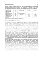
1. Introduction
This chapter deals with the problem of parameter identification of electrical machines to
achieve good performance of a control system. The development of an identification algorithm
is presented, which in this case is applied to Single-Phase Induction Motors, but could easily
be applied to other electrical machine. This scheme is based on a Robust Model Reference
Adaptive Controller and measurements of stator currents of a machine with standstill rotor.
From the obtained parameters, it is possible to design high performance controllers and
sensorless control for induction motors.
Single-phase induction motors (SPIM) are widely used in fractional and sub-fractional
horsepower applications, usually in locations where only single-phase energy supply is
available. In most of these applications the machine operates at constant frequency and is
fed directly from the AC grid with an ON/OFF starting procedure. In recent years, several
researchers have shown that the variable speed operation can enhance the SPIM’s efficiency
(Blaabjerg et al., 2004; Donlon et al., 2002). In addition, other researchers have developed high
performance drives for SPIM’s, using Field-Oriented Control (FOC) and sensorless techniques
(de Rossiter Correa et al., 2000; Vaez-Zadeh & Reicy, 2005; Vieira et al., 2009b). However,
the FOC associated with the sensorless technique demands accurate knowledge of electrical
motor parameters to achieve good performance.
A good deal of research has been carried out in the last several years on parameter estimation
of induction motors, mainly with regards to three-phase induction machines (Azzolin et al.,
2007; Koubaa, 2004; Ribeiro et al., 1995; Velez-Reyes et al., 1989).

However, few methods have been proposed for automatic estimation in single-phase
induction motors. One of them uses a classical method for electrical parameter identification
(Ojo & Omozusi, 2001), its implementation is onerous. In (Vieira et al., 2009a) a Recursive
Least Squares (RLS) identification algorithm is used to obtain machine parameters. The
identification results are good, although this method requires the design of filters to obtain
the variable derivative, which can be deteriorated by noises.
In order to solve these problems, this chapter details a closed-loop algorithm to estimate
the electrical parameters of a single-phase induction motor based on (Azzolin & Gründling,
A RMRAC Parameter Identification Algorithm
Applied to Induction Machines
8
lsq
L
sq
R
mq
L
q
d
N
rrd
N
ω f
lrq
L
sq
i
sq
v
rq

R
+-
+
-
+-
+
-
lsd
L
sd
R
md
L
d
q
N
rrq
N
ω f
lrd
L
sd
i
sd
v
rd
R
Fig. 1. Equivalent circuit of a SPIM.
2009). In (Azzolin & Gründling, 2009) a Robust Model Reference Adaptive Controller
(RMRAC) algorithm was used for parameter identification of three-phase induction motors.

The RMRAC algorithm eliminates the use of filters to obtain derivatives of the signals. Thus,
the objectives of this chapter are to apply the RMRAC algorithm in the electrical parameter
identification of a SPIM and make use of the robustness of the system in dealing with of noise
measurement.
As a result, the proposed parameter estimation procedure is divided into three steps:
(I) identification of the RMRAC controller gains;
(II) estimation of the transfer function coefficients of the induction motor at standstill;
(III) calculation of the stator resistance R
si
, rotor resistance R
ri
, stator inductance L
si
, rotor
inductance L
ri
and mutual inductance L
mi
using steps (I) and (II), where the index ”
i
”
express the axes q or d.
This chapter is organized as follows: Section 2 presents the induction machine model. A short
review of the RMRAC algorithm applied to the identification system is presented in sections 3
and 4. Section 5 describes the assumptions and equations of Model Reference Control (MRC)
while section 6 shows the proposed parameter identification algorithm. Sections 7 and 8
present the simulation and experimental results. Finally, chapter conclusions are presented
in section 9.
2. Mathematical model of a single phase induction motor
The SPIM equivalent circuit without the permanent split-capacitor can be represented by an

asymmetrical two-phase induction motor as shown in Fig. 1. In this figure L
lsi
and L
lri
are
the stator and rotor leakage inductances, ω
r
is the speed rotor, φ
ri
is the electromagnetic flux
and N
i
is the number of turns for auxiliary winding or axis d and for main winding or axis q.
The stator and rotor inductances are relationship with the leakage and mutual inductance as
a L
si
= L
lsi
+ L
mi
and L
ri
= L
lri
+ L
mi
, respectively.
From Fig. 1 and from (Krause et al., 1986) it is possible to derive the dynamical model of a
SPIM. The SPIM dynamical model in a stationary reference frame can be described by 1. In this
146

Electric Machines and Drives
equation
¯
σ
q
= L
sq
L
rq
− L
2
mq
,
¯
σ
d
= L
sd
L
rd
− L
2
md
, p is the poles pairs and n is the relationship
between the number of turns for auxiliary and for main winding N
d
/N
q
.
•

⎡
⎢
⎢
⎣
i
sq
i
sd
i
rq
i
rd
⎤
⎥
⎥
⎦
=
⎡
⎢
⎢
⎢
⎢
⎢
⎢
⎢
⎢
⎢
⎢
⎣
−

R
sq
L
rq
¯
σ
q
−pω
r
1
n
L
mq
L
md
¯
σ
q
R
rq
L
mq
¯
σ
q
−pω
r
1
n
L

rd
L
mq
¯
σ
q
pω
r
n
L
mq
L
md
¯
σ
d
−
L
rd
R
sd
¯
σ
d
pω
r
n
L
rq
L

md
¯
σ
d
R
rd
L
md
¯
σ
d
L
mq
R
sq
¯
σ
q
pω
r
1
n
L
sq
L
md
¯
σ
q
−

L
sq
R
rq
¯
σ
q
pω
r
1
n
L
sq
L
rd
¯
σ
q
−pω
r
n
L
sd
L
mq
¯
σ
d
L
md

R
sd
¯
σ
d
−pω
r
n
L
sd
L
rq
¯
σ
d
−
L
sd
R
rd
¯
σ
d
⎤
⎥
⎥
⎥
⎥
⎥
⎥

⎥
⎥
⎥
⎥
⎦
.(1)
.
⎡
⎢
⎢
⎣
i
sq
i
sd
i
rq
i
rd
⎤
⎥
⎥
⎦
+
⎡
⎢
⎢
⎢
⎢
⎢

⎢
⎢
⎢
⎢
⎢
⎣
L
rq
¯
σ
q
0
0
L
rd
¯
σ
d
−
L
mq
¯
σ
q
0
0
−
L
md
¯

σ
d
⎤
⎥
⎥
⎥
⎥
⎥
⎥
⎥
⎥
⎥
⎥
⎦

v
sq
v
sd

From equation 1 it is possible to obtain the transfer functions in the axes q and d at standstill
rotor (ω
r
= 0), where these equations are decoupled and presented in 2 and 3.
H
q
(
s
)
=

i
sq
(
s
)
v
sq
(
s
)
=
s
L
rq
¯
σ
q
+
R
rq
¯
σ
q
s
2
+ sp
q
+
R
rq

R
sq
¯
σ
q
,(2)
H
d
(
s
)
=
i
sd
(
s
)
v
sd
(
s
)
=
s
L
rd
¯
σ
d
+

R
rd
¯
σ
d
s
2
+ sp
d
+
R
rd
R
sd
¯
σ
d
,(3)
where
p
q
=
R
sq
L
rq
+ R
rq
L
sq

¯
σ
q
and p
d
=
R
sd
L
rd
+ R
rd
L
sd
¯
σ
d
.(4)
3. Identification system
The proposed electrical parameter identification system is shown in Fig. 2. This system is
based on a RMRAC algorithm used to generate the control action v
sq
by the difference between
the measured current i
sq
and the reference i
∗
sq
at standstill rotor. In this test the auxiliary
winding (or axis d) is open while the main winding (or axis q) is identified.

The dotted box in Fig. 2 is detailed in Fig. 3 where the RMRAC control law applied to q axis
is shown. In Fig. 3, the reference model and plant are given by
W
m
(s)=k
m
Z
m
(
s
)
R
m
(
s
)
,(5)
147
A RMRAC Parameter Identification Algorithm Applied to Induction Machines
IM
sq
v
0=
sd
v
RMRAC
q
sq
i
*

sq
i
0=
sd
i
Fig. 2. Block diagram of the RMRAC identification system.
()
p
Gs
()
m
Ws
r
1
e
m
y
p
y
p
u
+
+
+
+
+
-
()
()Λ
s

s
a
1
w
T
3
4
θ
θ
2
4
θ
θ
T
1
4
θ
θ
T
4
1
θ
s=- -
&
2
P
P ε
m
ξ
θθ

1
2
1
p
p
u
y
ω
ω
e
ü
ï
ï
ý
ï
ï
þ
()
*
sq
i
()
sq
v ()
sq
i
()
sqm
i
()

Λ( )
s
s
a
2
w
T
Fig. 3. RMRAC structure.
G
p
(s)=k
p
Z
p
(
s
)
R
p
(
s
)
.(6)
where Z
m
(s), R
m
(s), Z
p
(s) and R

p
(s) are monic polynomials and k
m
and k
p
are high frequency
gains.
The general idea behind RMRAC is to create a closed-loop controller with gains that can be
updated and change the response of the system. The output of the system y
p
is compared to a
desired response from a reference model y
m
. The controller gains vector θ =[θ

1
θ

2
θ
3
θ
4
]

is updated by a gradient algorithm based on e
1
error. The goal is that the gains converge to
ideal values that cause the plant response to match the response of the reference model. These
gains can be obtained by a gradient algorithm presented in (Ioannou & Sun, 1996; Ioannou &

Tsakalis, 1986) and described as follows. More details of RMRAC algorithms can be seen in
(Câmara & Gründling, 2004).
148
Electric Machines and Drives