Electric Machines and Drives part 9 potx

The procedure described in Fig. 2 and Fig. 3 is applied to parameter identification of the q axis
or transfer function 2. However, the same procedure is used for parameter identification of
the d axis or transfer function 3.
4. RMRAC gains adaptation algorithm
The gradient algorithm used to obtain the control law gains is given by
˙
θ
= −σPθ −
Pξ
m
2
ε,(7)
with
˙
m
= δ
0
m + δ
1



u
p


+


y
p



+ 1

, m(0) >
δ
1
δ
0
, δ
1
≥ 1, (8)
and
ξ
= W
m
(s)Iw,(9)
w
=[w

1
w

2
y
p
u
p
]


, (10)
w

1
, w

2
are auxiliary vectors, δ
0
, δ
1
are positive constants and δ
0
satisfies δ
0
+ δ
2
≤min(p
0
, q
0
),
q
0
∈
+
is such that the W
m
(s −q
0

) poles and the (F −q
0
I) eigenvalues are stable and δ
2
is a
positive constant. The sigma modification σ in 7 is given by
σ
=
⎧
⎪
⎪
⎨
⎪
⎪
⎩
0if

θ

<
M
0
σ
0


θ

M
0

−1

if M
0
≤

θ

<
2M
0
σ
0
if

θ

≥
2M
0
, (11)
where M
0
> θ
∗
 and σ
0
> 2μ
−2
/R

2
, R, μ ∈
+
are design parameters. In this case, the
parameters used in the implementation of the gradient algorithm are
⎧
⎪
⎪
⎪
⎪
⎨
⎪
⎪
⎪
⎪
⎩
δ
0
= 0.7
δ
1
= 1
δ
2
= 1
σ
0
= 0.1
M
0

= 10
, (12)
More details of design of the gradient algorithm can be seen in (Ioannou & Tsakalis, 1986). As
defined in (Lozano-Leal et al., 1990), the modified error in 7 is given by
ε
= e
1
+ θ

ξ −W
m
θ

w, (13)
or
ε
= φ

ξ + μη. (14)
When the ideal values of gains are identified and the plant model is well known, the plant can
be obtained by equation analysis of MRC algorithm described in the next section.
149
A RMRAC Parameter Identification Algorithm Applied to Induction Machines
2
4
()
Λ( )
s
θ
s

θ
a
T
r
+
+
+
+
3
4
θ
θ
4
1
θ
1
4
θ
θ
T
å
()
p
Gs
p
y
p
u
()
Λ( )

s
s
a
Fig. 4. MRC structure.
5. MRC analysis
The Model Reference Control (MRC) shown in Fig. 4 can be understood as a particular case
of RMRAC structure, which is presented in Fig. 3. This occurs after the convergence of the
controller gains when the gradient algorithm changes to the steady-state. It is important to
note that this analysis is only valid when the plant model is well known and free of unmodeled
dynamics and parametric variations.
To allow the analysis of the MRC structure, the plant and reference model must satisfy some
assumptions as verified in (Ioannou & Sun, 1996). These suppositions, which are also valid for
RMRAC, are given as follow:
Plant Assumptions:
P1. Z
p
(s) is a monic Hurwitz polynomial of degree m
p
;
P2. An upper bound n of the degree n
p
of R
p
(s);
P3. The relative degree n
∗
= n
p
−m
p

of G
p
(s);
P4. The signal of the high frequency gain k
p
is known.
Reference Model Assumptions:
M1. Z
m
(s), R
m
(s) are monic Hurwitz polynomials of degree q
m
, p
m
, respectively, where
p
m
≤ n;
M2. The relative degree n
∗
m
= p
m
− q
m
of W
m
(s) is the same as that of G
p

(s), i.e.,
n
∗
m
= n
∗
.
In Fig. 4 the feedback control law is
u
p
=
θ

1
θ
4
α
(
s
)
Λ
(
s
)
u
p
+
θ

2

θ
4
α
(
s
)
Λ
(
s
)
y
p
+
θ
3
θ
4
y
p
+
1
θ
4
r, (15)
and
α
(
s
)
Δ

= α
n−2
(
s
)
=

s
n−2
, s
n−3
, ,s,1


for n ≥ 2,
α
(
s
)
Δ
= 0forn = 1,
(16)
θ
3
, θ
4
∈
1
; θ


1
, θ

2
∈
n−1
are constant parameters to be designed and Λ(s) is an arbitrary
monic Hurwitz polynomial of degree n
−1 that contains Z
m
(s) as a factor, i.e.,
Λ
(
s
)
=
Λ
0
(
s
)
Z
m
(
s
)
, (17)
150
Electric Machines and Drives
which implies that Λ

0
(s) is monic, Hurwitz and of degree n
0
= n −1 − q
m
. The controller
parameter vector
θ
=

θ

1
θ

2
θ
3
θ
4


∈
2n
, (18)
is given so that the closed loop plant from r to y
p
is equal to W
m
(s). The I/O properties of the

closed-loop plant shown in Fig. 4 are described by the transfer function equation
y
p
= G
c
(s)r, (19)
where
G
c
(s)=
k
p
Z
p
Λ
2
Λ

θ
4
Λ −θ

1
α

R
p
−k
p
Z

p

θ

2
α + θ
3
Λ

, (20)
Now, the objective is to choose the controller gains so that the poles are stable and the
closed-loop transfer function G
c
(s)=W
m
(s), i.e.,
k
p
Z
p
Λ
2
Λ

θ
4
Λ −θ

1
α


R
p
−k
p
Z
p

θ

2
α + θ
3
Λ

= k
m
Z
m
R
m
. (21)
Thus, considering a system free of unmodeled dynamics, the plant coefficients can be known
by the MRC structure, i.e., k
p
, Z
p
(s) and R
p
(s) are given by 21 when the controller gains θ


1
,
θ

2
, θ
3
and θ
4
are known and W
m
(s) is previously defined.
6. Parameter identification using RMRAC
The proposed parameter estimation method is executed in three steps, described as follows:
6.1 First step: Convergence of controller gains vector
The proposed parameter identification method is shown in Fig. 2. In this figure the parameter
identification of q axis is shown, but the same procedure is performed for parameter
identification of d axis, one procedure at a time.
A Persistent Excitant (PE) reference current i
∗
sq
is applied at q axis of SPIM at standstill rotor.
The current i
sq
is measured and controlled by the RMRAC structure while i
sd
stays at null
value. The controller structure is detailed in Fig. 3. When e
1

goes to zero, the controller gains
go to an ideal value. Subsequently, the gradient algorithm is put in steady-state and the system
looks like the MRC structure given by Fig. 4. Therefore, the transfer function coefficients can
be found using equation 21.
6.2 Second step: Estimation of k
pi
, h
0i
, a
1i
and a
0i
This step consists of the determination of the Linear-Time-Invariant (LTI) model of the
induction motor. The machine is at standstill and the transfer functions given in 2 and 3 can
be generalized as follows
i
si
v
si
= k
pi
Z
pi
(
s
)
R
pi
(
s

)
=
k
pi
s + h
0i
s
2
+ sa
1i
+ a
0i
, (22)
where
k
pi
=
L
ri
¯
σ
i
, h
0i
=
R
ri
L
ri
, a

1i
= p
i
and a
0i
=
R
si
R
ri
¯
σ
i
, (23)
151
A RMRAC Parameter Identification Algorithm Applied to Induction Machines
The reference model given by 5 is rewritten as
W
m
(
s
)
=
k
m
Z
m
R
m
= k

m
s + z
0
s
2
+ p
1
s + p
0
, (24)
and from the plant and reference model assumptions results

m
p
= 1, n
p
= 2, n
∗
= 1,
q
m
= 1, p
m
= 2, n
∗
m
= 1,
(25)
The upper bound n is chosen equal to n
p

because the plant model is considered well known
and with n
= n
p
only one solution is guaranteed for the controller gains. Thus, the filters are
given by

Λ
(
s
)
=
Z
m
(
s
)
=
s + z
0
,
α
(
s
)
=
z
0
,
(26)

Assuming the complete convergence of controller gains, the plant coefficients are obtained
combining the equations 22, 24 and 26 in 21 and are given by
⎧
⎪
⎪
⎪
⎪
⎪
⎪
⎪
⎨
⎪
⎪
⎪
⎪
⎪
⎪
⎪
⎩
k
pi
= k
m
θ
4i
,
h
0i
=
z

0
θ
4i

θ
4i
−θ

1i

,
a
1i
= p
1
+ k
m
θ
3i
,
a
0i
= p
0
+ k
m
z
0

θ


2i
+ θ
3i

.
(27)
6.3 Third step: R
si
, R
ri
, L
si
, L
ri
and L
mi
calculation
Combining the equations 4, 23 and using the values obtained in 27 after the convergence of
the controller gains, we obtain the parameters of the induction motor:
⎧
⎪
⎪
⎪
⎪
⎪
⎪
⎪
⎪
⎪

⎪
⎪
⎪
⎪
⎨
⎪
⎪
⎪
⎪
⎪
⎪
⎪
⎪
⎪
⎪
⎪
⎪
⎪
⎩
ˆ
R
si
=
a
0i
k
pi
h
0i
,

ˆ
R
ri
=
a
1i
k
pi
−
ˆ
R
si
,
ˆ
L
si
=
ˆ
L
ri
=
ˆ
R
ri
h
0i
,
ˆ
L
mi

=

ˆ
L
2
si
−
ˆ
R
si
ˆ
R
ri
a
0i
.
(28)
In the numerical solution it-is considered that stator and rotor inductances have the same
values in each winding.
7. Simulation results
Simulations have been performed to evaluate the proposed method. The machine model given
by 1 was discretized by Euller technique under frequency of f
s
= 5kHz.TheSPIMwas
performed with a square wave reference of current and standstill rotor. The SPIM used is
a four-pole, 368W, 1610rpm, 220V/3.4A. The parameters of this motor obtained from classical
no-load and locked rotor tests are given in Table 1.
152
Electric Machines and Drives
R

sq
R
rq
L
mq
L
sq
7.00Ω 12.26Ω 0.2145H 0.2459H
R
sd
R
rd
L
md
L
sd
20.63Ω 28.01Ω 0.3370H 0.4264H
Table 1. Motor parameter obtained from classical tests.
650 650.1 650.2 650.3 650.4 650.5 650.6
−1.5
−1
−0.5
0
0.5
1
1.5
Time (s)
Output of reference model and plant

y
p
(i
sq
)
y
m
(i
sqm
)
Fig. 5. Plant and reference model output.
The reference model W
m
(s) is chosen so that the dynamic will be faster than plant output i
sq
.
Thus, the reference model is given by
W
m
(
s
)
=
180
s
+ 45
s
2
+ 180s + 8100
, (29)

The induction motor is started in accordance with Fig. 2 with a Persistent Excitant reference
current signal. A random noise was simulated to give nearly experimental conditions. Fig. 5
show the plant and reference model output after convergence of gains.
Fig. 6 shows the convergence of controller gains for parameter identification of q axis.
This figure shows that gains reach a final value after 600s, demonstrating that parameter
identification is possible. The gain convergence of d axis is shown in Fig. 7. Table 2 presents
the final value of controller gains for the q and d axes, respectively.
θ
1q
θ
2q
θ
3q
θ
4q
-0.0096 -1.0925 0.8332 -0.0950
θ
1d
θ
2d
θ
3d
θ
4d
-0.0164 -0.6429 0.6885 -0.0352
Table 2. Final value of controller gains obtained in simulation.
The parameters of SPIM are obtained by combining the final value of controller gains from
Table 2 with the equations 27, 28 and the reference model coefficients previously defined in
153
A RMRAC Parameter Identification Algorithm Applied to Induction Machines

0 100 200 300 400 500 600 700
−2
−1.5
−1
−0.5
0
0.5
1
Time (s)
Convergence of controller gains


θ
1q
θ
2q
θ
3q
θ
4q
Fig. 6. Convergence of controller gains vector for q axis.
0 100 200 300 400 500 600 700
−2
−1.5
−1
−0.5
0
0.5
1

Time (s)
Convergence of controller gains
θ
1d
θ
2d
θ
3d
θ
4d
Fig. 7. Convergence of controller gains vector for d axis.
equation 29. The results are shown in Table 3. It is possible to observe in simulation that the
electrical parameters converge to machine parameters, even with noise in the currents.
R
sq
R
rq
L
mq
L
sq
7.07Ω 12.21Ω 0.2150H 0.2462H
R
sd
R
rd
L
md
L

sd
20.22Ω 27.67Ω 0.3312H 0.4292H
Table 3. Motor parameter identified in simulation.
154
Electric Machines and Drives
0 100 200 300 400 500
−0.5
−0.4
−0.3
−0.2
−0.1
0
0.1
Time (s)
Convergence of controller gains


θ
1q
θ
2q
θ
3q
θ
4q
Fig. 8. Experimental convergence of controller gains for q axis.
8. Experimental results
This section presents experimental results obtained from the induction motor described in
simulation, whose electrical parameters obtained by classical no-load and locked rotor tests
are shown in Table 1. The drive system consists of a three-phase inverter controlled by

a TMS320F2812 DSP controller. The sampling period is the same used in the preceding
simulation.
Unlike the simulation, unmodeled dynamics by drive, sensors and filters, among others, are
included in the implementation. This implies that the plant model is a little different from
physical plant. As a result, there is a small error that is proportional to plant uncertainties
and is defined here as a residual error. The tracking error e
1
can be minimized by increasing
the gradient gain P. However, increasing P in order to eliminate the residual error can cause
divergence of controller gains and the system becomes unstable.
To overcome this problem a stopping condition was defined for the gain convergence. The
identified stator resistance
ˆ
R
si
was compared to measured stator resistance R
si
obtained from
measurements. Thus, the gradient gain P must be adjusted until the identified stator resistance
is equal to the stator resistance measurement.
Figure 8 presents the convergence of controller gains for q axis. The gains reach a final value
after 400s. Figure 9 presents the convergence of controller gains for d axis. The value of the
gain that resulted in
ˆ
R
si
= R
si
was P = 20I.
The plant output i

sq
and reference model output i
sqm
are shown in Fig. 10, after controller gain
convergence, where it is possible to see the residual error between the two curves. The final
values of controller gains, for axes q and d, are shown in Table 4.
The parameters of SPIM are obtained by combining the final value of controller gains of Table
4 with the equations 27, 28 and the reference model coefficients previously defined in equation
29. The results are shown in Table 5.
155
A RMRAC Parameter Identification Algorithm Applied to Induction Machines
0 100 200 300 400 500
−2
−1.5
−1
−0.5
0
0.5
Time (s)
Convergence of controller gains


θ
1d
θ
2d
θ
3d
θ
4d

Fig. 9. Experimental convergence of controller gains for d axis.
401 401.2 401.4 401.6 401.8 402
−2
−1.5
−1
−0.5
0
0.5
1
1.5
2
Time (s)
Output of reference model and plant


y
p
(i
sq
)
y
m
(i
sqm
)
Fig. 10. Experimental plant and reference model output.
θ
1q
θ
2q

θ
3q
θ
4q
0.0136 -0.558 -0.0555 -0.0423
θ
1d
θ
2d
θ
3d
θ
4d
0.0042 -0.6345 0.1560 -0.0207
Table 4. Final value of controller gains obtained in experimentation.
156
Electric Machines and Drives
R
sq
R
rq
L
mq
L
sq
6.9105Ω 15.4181Ω 0.1821H 0.2593H
R
sd
R
rd

L
md
L
sd
20.9438Ω 34.9016Ω 0.4926H 0.6447H
Table 5. Motor parameter identified in experimentation.
0 0.1 0.2 0.3 0.4 0.5 0.6 0.7
−2
−1.5
−1
−0.5
0
0.5
1
1.5
2
Time (s)
Measured and simulated currents


i
sq
(measured)
i
sq
(simulated)
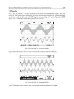
Fig. 11. Transient of comparison among measured and simulated currents from q axis.
8.1 Comparison for parameter validation
A comparative study was performed to validate the parameters obtained by the proposed
technique. The physical SPIM was fed by steps of 50V and 30Hz.Thecurrentsofmain

winding, auxiliary winding and speed rotor were measured.
Then, the dynamic model of SPIM given by 1 was simulated, using the parameters from Table
5, under the same conditions experimentally, i.e., steps of 50V and 30Hz. The measured rotor
speed was used in the simulation model to make it independent of mechanical parameters.
Thus, the simulated currents, from q and d windings, were compared with measured currents.
Figures 11 and 12 shows the transient currents from axis q and d, respectively, while Figures
13 and 14 shows the steady-state currents from axis q and d, respectively.
From Figures 11-14, it is clear that the simulated machine with the proposed parameters
presents similar behavior to the physical machine, both in transient and steady-state.
9. Conclusions
This chapter describes a method for the determination of electrical parameters of single phase
induction machines based on a RMRAC algorithm, which initially was used in three-phase
induction motor estimation in (Azzolin & Gründling, 2009). Using this methodology, it is
possible to obtain all electrical parameters of SPIM for the simulation and design of an high
performance control and sensorless SPIM drives. The main contribution of this proposed work
is the development of automated method to obtain all electric parameters of the induction
machines without the requirement of any previous test and derivative filters. Simulation
157
A RMRAC Parameter Identification Algorithm Applied to Induction Machines
0 0.1 0.2 0.3 0.4 0.5 0.6 0.7
−1
−0.5
0
0.5
1
Time (s)
Measured and simulated currents


i

sd
(measured)
i
sd
(simulated)
Fig. 12. Transient of comparison among measured and simulated currents from d axis.
0.5 0.52 0.54 0.56 0.58 0.6 0.62 0.64 0.66 0.68 0.7
−1.5
−1
−0.5
0
0.5
1
1.5
Time (s)
Measured and simulated currents


i
sq
(measured)
i
sq
(simulated)
Fig. 13. Steady-state of comparison among measured and simulated currents from q axis.
results demonstrate the convergence of the parameters to ideal values, even in the presence of
noise. Experimental results show that the parameters converge to different values in relation
to the classical tests shown in Table 1. However, the results presented in Figures 11-14 show
that the parameters obtained by proposed method present equivalent behavior to physical
machine.

158
Electric Machines and Drives
0.5 0.52 0.54 0.56 0.58 0.6 0.62 0.64 0.66 0.68 0.7
−1
−0.8
−0.6
−0.4
−0.2
0
0.2
0.4
0.6
0.8
1
Time (s)
Measured and simulated currents


i
sd
(measured)
i
sd
(simulated)
Fig. 14. Steady-state of comparison among measured and simulated currents from d axis.
10. References
Azzolin, R. & Gründling, H. (2009). A mrac parameter identification algorithm for three-phase
induction motors, Electric Machines and Drives C o nference, 2009. IEMDC ’09. IEEE
International, pp. 273 –278.
Azzolin, R., Martins, M., Michels, L. & Gründling, H. (2007). Parameter estimator of an

induction motor at standstill, Industrial Electronics, 2009. IECON ’09. 35th Annual
Conference of IEEE, pp. 152 – 157.
Blaabjerg, F., Lungeanu, F., Skaug, K. & Tonnes, M. (2004). Two-phase induction motor drives,
Industry Applications Magazine, IEEE 10(4): 24 – 32.
Câmara, H. & Gründling, H. (2004). A rmrac applied to speed control of an induction motor
without shaft encoder, Decision and Control, 2004. CDC. 43rd IEEE Conference on,Vol.4,
pp. 4429 – 4434 Vol.4.
de Rossiter Correa, M., Jacobina, C., Lima, A. & da Silva, E. (2000). Rotor-flux-oriented control
of a single-phase induction motor drive, Industrial Electronics, IEEE Transactions on
47(4): 832 –841.
Donlon, J., Achhammer, J., Iwamoto, H. & Iwasaki, M. (2002). Power modules for appliance
motor control, Industry Applications Magazine, IEEE 8(4): 26 –34.
Ioannou, P. & Sun, J. (n.d.). Robust Adaptive Control, Prentice Hall.
Ioannou, P. & Tsakalis, K. (1986). A robust direct adaptive controller, Automatic Control, IEEE
Transactions on 31(11): 1033 – 1043.
Koubaa, Y. (2004). Recursive identification of induction motor parameters, Simulation
Modelling Practice and Theory 12(5): 363 – 381.
URL: />ad5b99750423f5ff23
Krause, P., Wasynczuk, O. & Sudhoff, S. (n.d.). Analysis of Electric Machinery, NJ: IEEE Press.
159
A RMRAC Parameter Identification Algorithm Applied to Induction Machines
Lozano-Leal, R., Collado, J. & Mondie, S. (1990). Model reference robust adaptive control
without a priori knowledge of the high frequency gain, Automatic Control, IEEE
Transactions on 35(1): 71 –78.
Ojo, O. & Omozusi, O. (2001). Parameter estimation of single-phase induction machines,
Industry Applications Conference, 2001. Thirty-Sixth IAS Annual Meeting. Conference
Record of the 2001 IEEE.
Ribeiro, L., Jacobina, C. & Lima, A. (1995). Dynamic estimation of the induction machine
parameters and speed, Power Electronics Specialists Conference, 1995. P ESC ’95 Record.,
26th Annual IEEE, Vol. 2, pp. 1281 –1287 vol.2.

Vaez-Zadeh, S. & Reicy, S. (2005). Sensorless vector control of single-phase induction motor
drives, Electrical Machines and Systems, 2005. ICEMS 2005. Proceedings of the Eighth
International Conference on, Vol. 3, pp. 1838 –1842 Vol. 3.
Velez-Reyes, M., Minami, K. & Verghese, G. (1989). Recursive speed and parameter estimation
for induction machines, Industry Applications Society Annual Meeting, 1989., Conference
Record of the 1989 IEEE, pp. 607 –611 vol.1.
Vieira, R., Azzolin, R. & Gründling, H. (2009a). Parameter identification of a single-phase
induction motor using rls algorithm, Power Electronics Conference, 2009. C OBEP ’09.
Brazilian.
Vieira, R., Azzolin, R. & Gründling, H. (2009b). A sensorless single-phase induction motor
drive with a mrac controller, Industrial Electronics, 2009. IECON ’09. 35th Annual
Conference of IEEE, pp. 1003 –1008.
160
Electric Machines and Drives
9
Swarm Intelligence Based Controller
for Electric Machines and Hybrid
Electric Vehicles Applications
Omar Hegazy
1
, Amr Amin
2
, and Joeri Van Mierlo
1

1
Faculty of Engineering Sciences Department of ETEC- Vrije Universiteit Brussel,
2
Power and Electrical Machines Department, Faculty of Engineering – Helwan University,
1

Belgium
2
Egypt
1. Introduction
Swarm Intelligence in the form of Particle Swarm Optimization (PSO) has potential
applications in electric drives. The excellent characteristics of PSO may be successfully
used to optimize the performance of electric machines and electric drives in many
aspects. It is estimated that, electric machines consume more than 50% of the world
electric energy generated. Improving efficiency in electric drives is important, mainly,
for two reasons: economic saving and reduction of environmental pollution. Induction
motors have a high efficiency at rated speed and torque. However, at light loads, the
iron losses increase dramatically, reducing considerably the efficiency. Swarm
intelligence is used to optimize the performance of three applications; these
applications are represented as follows:
• Losses Minimization of two asymmetrical windings induction motor
• Maximum efficiency and minimum operating cost of three-phase induction motor
• Optimal electric drive system for fuel cell hybrid electric vehicles.
In this chapter, a field-oriented controller that is based on Particle Swarm Optimization is
presented. In this system, the speed control of two asymmetrical windings induction motor
is achieved while maintaining maximum efficiency of the motor. PSO selects the optimal
rotor flux level at each operating point. In addition, the electromagnetic torque is also
improved while maintaining a fast dynamic response. A novel approach is used to evaluate
the optimal rotor flux level by using Particle Swarm Optimization. PSO method is a member
of the wide category of Swarm Intelligence methods (SI). The swarm intelligence is based on
real life observations of social animals (usually insects), it is more flexibility and robust than
any traditional optimization methods. PSO algorithm searches for global optimization for
nonlinear problems with multi-objective. There are two speed control strategies explained in
the next sections. These are field-oriented controller (FOC), and FOC based on PSO. The
strategies are implemented mathematically and experimental. The simulation and
experimental results have demonstrated that the FOC based on PSO method saves more

energy than the conventional FOC method.
Electric Machines and Drives

162
In this chapter, another application of PSO for losses and operating cost minimization
control is presented for the induction motor drives. Two strategies for induction motor
speed control are proposed. These strategies are maximum efficiency strategy (MES), based
PSO, and minimum operating cost Strategy. The proposed technique is based on the
principle that the flux level in a machine can be adjusted to give the minimum amount of
losses and minimum operating cost for a given value of speed and load torque.
In the demonstrated systems, the powertrain components sizing and the power control
strategy are the only adjustable parameters to achieve optimal power sharing between
sources and optimal design with minimum cost, minimum fuel consumption, and
maximum efficiency for Electric Vehicles (EVs) and Hybrid Electric Vehicles (HEVs). Their
selection greatly influences the performance of the drive system in Hybrid Electric Vehicles
applications. In this section, the design and power management control are investigated and
optimized by using Particle Swarm Optimization.
2. Losses minimization of two asymmetrical windings induction motor
In this section, a field orientation based on Particle Swarm Optimization (PSO) is applied to
control the speed of two-asymmetrical windings induction motor. The maximum efficiency
of the motor is obtained by the evaluation of optimal rotor flux at each operating point. In
addition, the electro-magnetic torque is also improved while maintaining a fast dynamic
response. In this section, a novel approach is used to evaluate the optimal rotor flux level.
This approach is based on Particle Swarm Optimization (PSO). This section presents two
speed control strategies. These are field-oriented controller (FOC) and FOC based on PSO.
The strategies are implemented mathematically and experimental. The simulation and
experimental results have demonstrated that the FOC based on PSO method saves more
energy than the conventional FOC method [Hegazy, 2006; Amin et al., 2007; Amin et al.,
2009]. The two asymmetrical windings induction motor is treated as a two-phase induction
motor (TPIM). It is used in many low power applications, where three–phase supply is not

readily available. This type of motor runs at an efficiency range of 50% to 65% at rated
operating conditions.
The conventional field-oriented controller normally operates at rated flux at any values with
its torque range. When the load is reduced considerably, the core losses become so high
causing poor efficiency. If significant energy savings are required, it is necessary to optimize
the efficiency of the motor. The optimum efficiency is obtained by the evaluation of the
optimal rotor flux level. This flux level is varied according to the torque and the speed of the
operating point.
PSO is applied to evaluate the optimal flux. It has the straightforward goal of minimizing
the total losses for a given load and speed. It is shown that the efficiency is reasonably close
to optimal.
2.1 Mathematical model of the motor
The d-q model of an unsymmetrical windings induction motor in a stationary reference
frame can be used for a dynamic analysis. This model can take in account the core losses.
The d-q model as applied to TPIM is described in [Hegazy, 2006; Amin et al., 2009]. The
equivalent circuit is shown in Fig. 1.
Swarm Intelligence Based Controller for
Electric Machines and Hybrid Electric Vehicles Applications

163
r
M
L
lM
L
mq
L
lr
+
-

(1/k)
ω
r
λ
dr
+
-
V
qs
r
r
i
qs
i
qr
R
qf e
i
qf e
r
A
L
lA
L
md
L
lR
+
-
k

ω
r
λ
qr
+
-
V
ds
i
ds
i
dr
R
df e
i
df e
r
R

Fig. 1. The d-q axes two-phase induction motor Equivalent circuit with iron losses.
The machine model may be expressed by the following voltage and flux equations:
Voltage Equations (1):

q
sm
q
s
q
s
vrip

λ
=
+ (1)

ds a ds ds
vrip
λ
=+
(2)

0(1/)*
r
q
rrdr
q
r
ri k p
ω
λλ
=
−+ (3)

0*
Rds r
q
rdr
ri k
p
ω
λλ

=
++ (4)
0()
qf
e
qf
em
qq
s
q
r
qf
e
iR L pi pi pi
=
−+ +− (5)
0()
d
f
ed
f
emdds drd
f
e
iR L pi pi pi
=
−+ +− (6)
Flux Equations:
()
q

slm
q
sm
qq
s
q
r
qf
e
Li L i i i
λ
=
++− (7)
()
ds la ds md ds dr d
f
e
Li L i i i
λ
=
++− (8)
Electric Machines and Drives

164

()
q
rlr
q
rm

qq
s
q
r
qf
e
Li L i i i
λ
=
++−
(9)
()
dr lR dr md ds dr d
f
e
Li L i i i
λ
=
++− (10)
Electrical torque equation is expressed as:

1
(( ) ( )
2
m
q
dr
q
s
q

r
qf
emd
q
rds dr
qf
e
P
Te kL i i i i L i i i i
k
=+−−+−
(11)

lmrmr
Te T j p B
ω
ω
−
=+ (12)
2.2 Field-Oriented Controller [FOC]
The stator windings of the motor are unbalanced. The machine parameters differ from the d
axis to the q axis. The waveform of the electromagnetic torque demonstrates the unbalance
of the system. The torque in equation (11) contains an AC term; it can be observed that two
values are presented for the referred magnetizing inductance. It is possible to eliminate the
AC term of electro-magnetic torque by an appropriate control of the stator currents.
However, these relations are valid only in linear conditions. Furthermore, the model is
implemented using a non-referred equivalent circuit, which presumes some complicated
measurement of the magnetizing mutual inductance of the stator and the rotor circuits.
The indirect field-oriented control scheme is the most popular scheme for field-oriented
controllers. It provides decoupling between the torque and the flux currents. The electric

torque must be a function of the stator currents and rotor flux in synchronous reference
frame [Popescu & Navrapescu, 2000]. Assuming that the stator currents can be imposed as:

1
ss
ds ds
ii
=
(13)

1
ss
q
s
q
s
iki=
(14)
Where:
k= M
srd
/ M
srq

2
dr qr
ss ss
e sqr qs sdr ds
r
P

TMiMi
L
λλ
⎡
⎤
=−
⎣
⎦
(15)
By substituting the variables
i
ds
, and i
qs
by auxiliary variables i
ds1
, and i
qs1
into (15) the torque
can be expressed by

11
2
qs dr ds qr
ss ss
sdr
e
r
PM
Tii

L
λλ
⎡
⎤
=−
⎣
⎦
(16)
In synchronous reference frame, the electromagnetic torque is expressed as:

11
2
qs dr ds qr
ee ee
sdr
e
r
PM
Tii
L
λλ
⎡
⎤
=−
⎣
⎦
(17)

1
2

qs r
ee
sdr
e
r
PM
Ti
L
λ
⎡
⎤
=
⎣
⎦
(18)
Swarm Intelligence Based Controller for
Electric Machines and Hybrid Electric Vehicles Applications

165

1
e
e
r
ds
sdr
i
M
λ
= (19)

1
*
qs
e
sdr
er
rr
M
i
ωω
τλ
−= (20)
2.3 Synchronous reference frame for losses model
It is very complex to find the losses expression for the two asymmetrical windings induction
motor with losses model. In this section, a simplified induction motor model with iron
losses will be developed. For this purpose, it is necessary to transform all machine variables
to the synchronous reference frame. The voltage equations are written in expanded form as
follows [Hegazy, 2006; Amin et al., 2006; Amin et al., 2009]:

()
ee
qs qm
ee e e
q
sm
q
slm m
q
elads mddm

di di
vriL L LiLi
dt dt
ω
=+ + + +
(21)

()
ee
ee e e
ds dm
ds a ds la md e lm
q
sm
qq
m
di di
vriL L LiLi
dt dt
ω
=+ + − + (22)

0()
ee
qr qm
eee
sl
r
q
rlr m

q
lR dr md dm
di di
ri L L L i L i
dt dt k
ω
=+ + + + (23)

0*()
ee
eee
dr dm
Rdr lR md sl lr
q
rm
qq
m
di di
ri L L k Li L i
dt dt
ω
=+ + − + (24)

eee e
q
s
q
r
qf
e

q
m
iii i+= + (25)

eee e
ds dr d
f
edm
iii i+=+ (26)

elrmqs
ee
dm
q
s
r
LL
vi
L
ω
=− (27)

ee
q
memdsds
vLi
ω
= (28)
Where:
e

e
qm
ee
dm
dfe dfe
qfe dfe
v
v
i;i
RR
==
The losses in the motor are mainly:
a.
Stator copper losses,
b.
Rotor copper losses,
c.
Core losses, and
Electric Machines and Drives

166
d. Friction losses
The total electrical losses can be expressed as follows
P
losses
= P
cu1
+ P
cu2
+P

core
(29)
Where:
P
cu1
: Stator copper losses
P
cu2
: Rotor copper losses
P
core
: Core losses
The stator copper losses of the two asymmetrical windings induction motor are caused by
electric currents flowing through the stator windings. The core losses of the motor are
produced from the hysteresis and eddy currents in the stator. The total electrical losses of
motor can be rewritten as:

2
2
222 2
e
e
qm
eee e
dm
losses m qs a ds r qr R dr
qf
ed
f
e

v
v
P riririri
RR
=+++++ (30)
The total electrical losses are obtained as follows:

2222
22 22 2
22 2 2
22
r mqs e lr mqs
er emds r
losses m a
qfe
rrd
f
emds
mds
r
rL L L
TL L
Pr r
R
LLR L
L
P
K
ω
ω

λ
λ
⎛⎞
⎜⎟
⎡⎤
⎛⎞
⎜⎟
⎢⎥
⎜⎟
=+ + ++
⎜⎟
⎜⎟
⎢⎥
⎛⎞
⎝⎠
⎣⎦
⎜⎟
⎜⎟
⎜⎟
⎝⎠
⎝⎠
(31)

2
2*
*
er
sl
r
Tr

P
ω
λ
= (32)
Where:
ω
e
= ω
r
+ ω
sl
, and ω
sl
is the slip speed (rad/sec).
Equation (31) is the electrical losses formula, which depends on rotor flux (λ
r
) according to
operating point (speed and load torque). The total losses of the motor (
losses
TP ) are given
as follows:

losses losses Fric in out
TP P P P - P
=
+= (33)

losses
Efficiency ( )
TP

out
out
P
P
η

=
+
(34)
Where:
Friction power losses = F ∗ω
r
2
, and
Output power (P
out
) = T
L
∗ω
r
.
2.4 Losses minimization control scheme
The equation (33) is the cost function, the total losses, which depends on rotor flux (λr)
according to the operating point. Figure 2 presents the distribution of losses in motor and its
variation with the flux. As the flux reduces from the rated value, the core losses decrease,
Swarm Intelligence Based Controller for
Electric Machines and Hybrid Electric Vehicles Applications

167
but the motor copper losses increase. However, the total losses decrease to a minimum value

and then increase again. It is desirable to set the rotor flux at the optimal value, so that the
efficiency is optimum [Hegazy, 2006; Amin et al., 2006; Amin et al., 2009].


Fig. 2. Losses variation of the motor with varying flux
PSO is applied to evaluate the optimal flux that minimizes the motor losses. The problem
can be formulated as follows:

losses L
minimize TP ( r,T , )
r
λ
ω
=Γ
(35)
2.4.1 Particle Swarm Optimization (PSO)
Particle swarm optimization (PSO) was originally designed and introduced by Eberhart and
Kennedy [Ebarhart, Kennedy, 1995; Ebarhart, Kennedy, 2001]. Particle Swarm Optimization
(PSO) is an evolutionary computation technique (a search method based on a nature
system). It can be used to solve a wide range of optimization problems. Most of the
problems that can be solved using Genetic Algorithms (GA) could be solved by PSO. For
example, neural network training and nonlinear optimization problems with continuous
variables can be easily achieved by PSO [Ebarhart, Kennedy, 2001]. It can be easily
expanded to treat problems with discrete variables.
The system initially has a population of random solutions. Each potential solution, called a
particle. Each particle is given a random velocity and is flown through the problem space.
The particles have memory and each particle keeps track of its previous best position (call
the pbest) and with its corresponding fitness. There exit a number of pbest for the respective
particles in the swarm and the particle with greatest fitness is called the global best (gbest)
of the swarm. PSO can be represented by the concept of velocity and position. The Velocity

of each agent can be modified by the following equations: (36 & 38):

k1
11 22
v*()*()
kk k
ii i
wv cr pbests cr gbests
+
=+ −+ − (36)
Electric Machines and Drives

168
Are
all possible operating
conditions optimized
varying the rotor
flux level using
PSO
Run the Simulik model of two asymmetrical
windings induction motor with losses
Det ermination of the new
operation conditions
(speed and torque)
Read motor parameters
Start
calc ulation of the c os t
function
Is
the value of

the cost
function is
minimum
?
No
set this value as optimum point
and record the corresponding
optimum values of the efficiency
and the rotor flux load
End
Yes
No
Yes
Calculation of motor currents

Fig. 3. The flowchart of the execution of the PSO [Hegazy, 2006)