Hydrodynamics Optimizing Methods and Tools Part 9 ppt
Bạn đang xem bản rút gọn của tài liệu. Xem và tải ngay bản đầy đủ của tài liệu tại đây (3.69 MB, 30 trang )
Hydrodynamics – Optimizing Methods and Tools
228
The F/E system was represented as a network of interconnected component elements, namely:
Reservoirs, representing the lock chambers, WSBs, the lake, and the oceans. Level-Area
relations were specified for each one of them. The lake and oceans were considered as
infinite area constant level reservoirs.
Rigid rectangular pipes, representing primary and secondary culverts, WSB conduits,
etc. The calculation of friction losses was made using Darcy-Weisbach and Colebrook-
White equations, as a function of the flow Reynolds number and the effective roughness
height of the conduit walls.
Local energy losses parameterized with a cross-section area and a head loss coefficient,
representing most of the special hydraulic components, such as bends, bifurcations,
transitions, etc.
Local energy losses expressed as laws for cross-section area and head loss coefficient in
terms of a control parameter, representing valves for which the control parameter is the
aperture.
2.3 Numerical modeling of physical model
The Third Set of Locks has been subject to physical modeling, both during the development
of the conceptual design, and later during the design for the final project. Both physical
models where commissioned to the Compagnie Nationale du Rhône (CNR), Lyon, France.
The physical models were built at a 1/30 scale, comprising 2 chambers and one set of three
WSBs. Extensive tests were made for various normal and special operations, measuring
water levels, discharges, pressures and water slopes in the chambers. Some tests included
the presence of a design vessel model, measuring hydraulic longitudinal and transversal
forces over its hull. Based on these tests, a correlation between forces on the ship, and water
surface slopes in the chamber in the absence of the ship (easier to measure and allegedly
more repeatable), was established. This correlation was used to impose maximum values to
the longitudinal and lateral water surface slopes, as contractual requirements.
The flow in the hydraulic model was numerically simulated. Real physical dimensions of
the physical model components (culverts, conduits, chambers) were used.
Local head loss coefficients for the special hydraulic components were obtained through
steady CFD modeling (see Section 3 for more details on CFD modeling), by calculating the
difference between upstream and downstream mechanical energy, and subtracting energy
losses due to wall friction. Most parts of the physical model were made out of acrylic (with a
0.025 mm roughness height), which behaves as a hydraulically smooth surface, for which
the roughness height is completely submerged within the viscous sublayer (White, 1974).
Some of the special hydraulic components, though, were built with Styrofoam (enclosed
inside of acrylic boxes), as the initial expectations were that many alternative geometries
would have to be tested, so this system would allow swapping with relative ease (very few
alternatives were finally tested, due the great success of the optimization process carried out
with CFD models). As it was later demonstrated that Styrofoam behaves as hydraulically
rough at the physical model scale, most of it had to be coated with a low roughness layer of
paint in order to avoid a spurious response (a scale effect in itself).
The results obtained with the numerical model (water levels, discharges, pressures) showed
a very good agreement with physical model measurements, for different operations and
conditions. As an illustration, Figs 2.3 and 2.4 show comparisons for a typical Lock to Lock
operation, with maximum initial head difference. All comparisons are presented with
results scaled up to prototype dimensions.
Interaction Between Hydraulic and Numerical Models for the Design of Hydraulic Structures
229
0%
25%
50%
75%
100%
0
50
100
150
200
250
300
350
400
450
0 60 120 180 240 300 360 420 480 540 600 660 720
Valve Aperture (%)
Main Culvert Dischage (m3/s)
Time (secs)
Physical Model - Far Side Mathematical Model - Far Side Valve Aperture
Fig. 2.3. Comparison of physical and numerical models: Discharge in the Main Culvert, for a
Lock to Lock operation with 21 m of initial head difference.
0%
20%
40%
60%
80%
100%
-4
-2
0
2
4
6
8
10
12
14
16
18
0 60 120 180 240 300 360 420 480 540 600 660 720
Valve Aperture (%)
Water Level (mPLD)
Time (secs)
Physical Model Mathematical Model Valve Aperture
Fig. 2.4. Comparison of physical and numerical models: Water levels in the chambers, for a
Lock to Lock operation with 21 m of initial head difference.
Hydrodynamics – Optimizing Methods and Tools
230
2.4 Numerical modeling of the prototype
Practical knowledge exists about the discrepancies between F/E times as measured in a
physical model and those effectively occurring at the prototype. For instance, USACE
manual on hydraulic design of navigation locks (2006) states:
”A prototype lock filling-and-emptying system is normally more efficient than
predicted by its model” ”The difference in efficiency is acceptable as far as most of the
modeled quantities are concerned (hawser forces, for example) and can be
accommodated empirically for others (filling time and over travel, specifically).”
In the specific commentaries about F/E times, it suggests quantitative corrections:
”General guidance is that the operation time with rapid valving should be reduced
from the model values by about 10 percent for small locks (600 ft or less) with short
culverts; about 15 percent for small locks with longer, more complex culvert systems;
and about 20 percent for small locks (Lower Granite, for example) or large locks having
extremely long culvert systems.”
The alternative, rigorous strategy proposed in the present paper is to numerically simulate
the flow in the prototype. This means using the physical dimensions of the prototype, the
corresponding local head loss coefficients for the special hydraulic components, and the
roughness height for concrete. Though the concrete wall also behaves as hydraulically
smooth, the friction coefficient for smooth pipes is a function of the flow Reynolds number,
as indicated by the “smooth pipe” curve in the Moody chart (Fig. 2.5).
Fig. 2.5. Friction coefficient as a function of Reynolds number (Moody chart)
Interaction Between Hydraulic and Numerical Models for the Design of Hydraulic Structures
231
For example, the Reynolds number in the primary culvert (in which most of the friction losses
are produced) changes in time following the flow hydrograph, from zero to the peak
discharge, and back to zero again. The peak discharge for 21 m initial head difference in a
Lock to Lock operation is around 425 m
3
/s (the corresponding flow velocity is 7.87 m/s). This
leads to a Reynolds number of around 6.5 10
7
for the prototype. When scaled to the physical
model, the Reynolds number is only 3.9 10
5
, i.e., a drop of more than two orders of magnitude.
The associated friction coefficients are then below 0.008 for the prototype, and about 0.014 for
the physical model. The consequently higher friction losses produced in the physical model,
exclusively due to scale effects, reduce the flow velocities, then increasing the F/E times.
The numerical model contemplates the variation of frictional losses with the Reynolds
number. Hence, it allows to be used in order to extrapolate the physical model results to
those expected for the prototype, overcoming the distortion introduced by scale effects in
the physical model results.
For the Panama Canal Third Set of Lock, the validated 1D model was scaled up to prototype
dimensions. Variations in local head loss coefficients, indicated by 3D models, were also
introduced. Relatively little effects were observed in the simulations because of the change
in local head loss coefficients. On the contrary, friction losses decreased significantly, as
already explained. Consequently, for a typical Lock to Lock operation with maximum initial
head difference, F/E times showed a 10% decrease (61 seconds) (Fig. 2.6).
0%
20%
40%
60%
80%
100%
-4
-2
0
2
4
6
8
10
12
14
16
18
0 60 120 180 240 300 360 420 480 540 600 660 720
Valve Aperture (%)
Water Level (mPLD)
Time (secs)
Prototype Scale Physical Model Scale Valve Aperture Series4
Fig. 2.6. Comparison of physical model scale and prototype scale numerical models: Water
levels in the chambers, for a Lock to Lock operation with 21 m of initial head difference.
Additionally, a 5% increase in the peak discharge of the main culverts was also observed
(Fig. 2.7). This has an effect over the pressures on the vena contracta, downstream of the
main culvert valves (Fig. 2.8), which had to be contemplated during the design stage, as air
intrusion had to be avoided (for contractual reasons), and because piezometric levels
downstream of the valves were close to the roof level of the culvert for various special
operating conditions. So avoiding scale effects was also significant to correctly deal with
these two limitations.
Hydrodynamics – Optimizing Methods and Tools
232
0%
25%
50%
75%
100%
0
50
100
150
200
250
300
350
400
450
0 60 120 180 240 300 360 420 480 540 600 660 720
Valve Aperture (%)
Main Culvert Dischage (m3/s)
Time (secs)
Culvert Discharge - Physical Model Scale Culvert Discharge - Prototype Scale
Valve Aperture - Physical Model Scale Valve Aperture - Prototype Scale
Fig. 2.7. Comparison of physical model scale and prototype scale numerical models:
Discharge in the Far Main Culvert, for a Lock to Lock operation with 21 m of initial head
difference.
0%
20%
40%
60%
80%
100%
120%
-16
-14
-12
-10
-8
-6
-4
-2
0
2
4
6
8
0 60 120 180 240 300 360 420
Valve Aperture (%)
Piezometric Level (mPLD)
Time (sec)
Prototype Scale - Piezometric Level Physical Model Scale - Piezometric Level Valves
Culvert Roof Elevation -7.13 mPLD
Culvert Sill Elevation -13.63 mPLD
Fig. 2.8. Comparison of physical model scale and prototype scale numerical models:
Piezometric level at the vena contracta, for a Lock to Lock operation with 21 m of initial
head difference.
Interaction Between Hydraulic and Numerical Models for the Design of Hydraulic Structures
233
3. Free surface oscillations
Free surface oscillations in the lock chambers leads to forces in the hawsers. Based on results
from the physical model constructed during the development of the conceptual design, a
correlation was found between these forces and the free surface slope in the absence of the
vessel, as already mentioned in Section 2. Hence, the free surface slope was used as an
indicator for the hawser forces. As a design restriction, a maximum value of 0.14 ‰ was
contractually established for the longitudinal water surface slope.
3.1 Description and modeling of phenomenon
Free surface oscillations in the lock chambers are triggered by asymmetries both in the flow
distribution among ports, and in the geometry of the chambers (Figure 3.1).
a) Flow distribution according to 1D model
b) Plan view of chamber
Fig. 3.1. Asymmetries which trigger free surface oscillations.
A 2D (vertically averaged) hydrodynamic model, based on code HIDROBID II developed at
INA (Menéndez, 1990), was used to simulate the surface waves. It was driven by the inflow
from the ports, specified as boundary conditions through time series for each one of them,
that were obtained with the 1D model described in the Section 2.
Fig. 3.2 shows the comparison between the calculated longitudinal free surface slope (using
the dimensions of the physical model) and the recorded one at the physical model, for a case
Hydrodynamics – Optimizing Methods and Tools
234
with a relatively low initial head difference (9 m in prototype units) between the Lower
Chamber and the Ocean. The agreement is considered as very good, taking into account that
the numerical model does not include the resolution of turbulent scales (which introduce a
smaller-amplitude, higher-frequency oscillation riding on the basic oscillation).
0.00
0.25
0.50
0.75
1.00
-0.140
-0.105
-0.070
-0.035
0.000
0.035
0.070
0.105
0.140
0 60 120 180 240 300 360 420 480 540 600
Valve Opening ratio
Longitudinal Water Surface Slope (o/oo)
Time (seconds)
Physical Model Numerical Model Valve Opening
Fig. 3.2. Longitudinal water surface slope using 1D model input. Low initial head difference.
However, the 2D model completely fails to correctly predict the longitudinal free surface
slope for higher initial head differences, as observed in Fig. 3.3 for a Lock to Lock operation
with an initial head difference of 21 m. More specifically, the recorded oscillation indicates a
quite more irregular response, with a much higher amplitude than the one calculated with the
0.00
0.25
0.50
0.75
1.00
-0.140
-0.105
-0.070
-0.035
0.000
0.035
0.070
0.105
0.140
0 60 120 180 240 300 360 420 480 540 600
Valve Opening ratio
Longitudinal Water Surface Slope (o/oo)
Time (seconds)
Physical Model Numerical Model Valve Opening
Fig. 3.3. Longitudinal water surface slope using 1D model input. High initial head
difference.
Interaction Between Hydraulic and Numerical Models for the Design of Hydraulic Structures
235
numerical model. This indicates that turbulence scales are exerting a significant influence, so a
more elaborated theoretical approach is needed. Hence, 3D modeling of the combination
Central Connection + Secondary Culvert + Ports + Lock Chamber (actually, only half of the
chamber, assuming that the flow is symmetrical with respect to the longitudinal axis) was
undertaken using a Large-Eddy Simulation (LES) approach (Sagaut, 2001).
3.2 Improved theoretical approach
As sub-grid scale (SGS) model for the LES approach, a sub-grid kinetic energy equation
eddy viscosity model was used (Sagaut, 2001). Deardorff’s method was selected to define
the filter cutoff length (Sagaut, 2001). A wall model was considered to treat the boundary
conditions at solid borders; Spalding law-of-the-wall – which encompasses the logarithmic
law (overlap region), but it holds deeper into the inner layer – was selected for the velocity
(White, 1974), while a zero normal gradient condition was taken for the remaining variables.
At the inflow boundary, in addition to the ensemble-averaged velocity (which arises from
the 1D model), the amplitude of the stochastic components were provided (Sagaut, 2001):
4% for the longitudinal component, and 1.3% for the transversal one, values associated to
a fully developed flow, very appropriate for the present problem; additionally, a
weighted average of the previous and present generated stochastic components was
imposed in order to add some temporal correlation; for the turbulent kinetic energy, a
zero normal gradient was taken. For the free surface at the Chamber, the rigid-lid
approximation was used, where uniform pressure was imposed, together with zero
normal gradient conditions for the remaining quantities. The model was implemented
using OpenFOAM (Open Field Operation And Manipulation), an open source toolbox for
the development of customizable numerical solvers and utilities for the solution of
continuum mechanics problems (Weller et al., 1998). The model solves the integral form of
the conservation equations using a finite volume, cell centered approach in the spirit of
Rhie and Chow (1983). PISO (Pressure Implicit with Splitting of Operators) algorithm is
used for time marching (Ferziger & Peric, 2001).
Fig. 3.4 presents a view of the model domain. The computational mesh was composed by 1.5
million elements. Special considerations were made for the mesh near the wall, as the center
of the first cell has to lie within a distance range to the wall – 30 y+ 300 – to rigurously
apply the logaritmic velocity profile as boundary condition (Sagaut, 2001). Typical
computing times for stabilization with a steady discharge, in a Core i7 PC running 8 parallel
processes, were 3 to 8 days. When complete hydroghaphs were simulated (of approximately
550 secs), 15 to 30 days of computing time were required. By parallelizing the simulation
using more than one PC, computing times were reduced, though non-linearly.
Fig. 3.4. Model domain for 3D model.
Hydrodynamics – Optimizing Methods and Tools
236
Note that the rigid-lid approximation implies that the free surface oscillations are not solved
by the 3D model; this was done in order to avoid extremely high computing times. Instead,
the 3D model provided the time series of the flow discharge for each port, which were used
to drive the 2D model of the chamber. Alternatively (and less costly in post-processing), the
time series of the discharges at the U and S branches of the Central Connection, provided by
the 3D model, were used to feed the 1D model, from which the discharge distribution
among ports was obtained, and used to feed the 2D model.
Fig. 3.5 shows the longitudinal water surface slope obtained with the two approaches (using
the dimensions of the physical model), and their comparison with the results from the
physical model, for the high initial head difference case. It is observed that both numerical
simulations are now able to capture the high amplitude oscillations, indicating that large
eddies must be responsible for this amplification phenomenon. Note that the numerical
results with input straight from the 3D model show oscillations, associated to large eddies,
which are not present in the ones with input through the 1D model (which filters out those
oscillations), but they are quite compatible between them.
-0.14
-0.105
-0.07
-0.035
0
0.035
0.07
0.105
0.14
0 60 120 180 240 300 360 420 480 540 600
Longitudinal Water Surface Slope (o/oo)
Time (seconds)
Physical Model From 3D Numerical Model Through 1D Numerical Model
Fig. 3.5. Longitudinal water surface slope using 3D-LES model input. High initial head
difference.
The differences between the numerical results and the measurements at the physical model
are due essentially to the variability of the system reponse (variations in amplitude and
phase of the oscillations), under the same driving conditions, due to the stochastic nature of
turbulence. This was verified both experimentally (Fig. 3.6a) and numerically (Fig. 3.6b) by
repeating the same test (in the case of the numerical model, using the ‘through 1D model‘
approach, and different initializations for the stochastic number generator). This behavior
puts a limit to the degree of agreement that can be attained between the results from the
numerical and physical models. In any case, the maximum amplitudes for any of the
experimental or numerical realizations are relatively consistent among them.
Interaction Between Hydraulic and Numerical Models for the Design of Hydraulic Structures
237
-0.140
-0.105
-0.070
-0.035
0.000
0.035
0.070
0.105
0.140
0 60 120 180 240 300 360 420 480 540 600
Longitudinal Water Surface Slope (o/oo)
Time (seconds)
Test 1 Test 2 Test 3
a) Experimental realizations
-0.14
-0.105
-0.07
-0.035
0
0.035
0.07
0.105
0.14
0 60 120 180 240 300 360 420 480 540 600
Longitudinal Water Surface Slope (o/oo)
Time (seconds)
Physical Model Simulation 1 Simulation 2
b) Numerical realizations
Fig. 3.6. Variability of longitudinal water surface slope. High initial head difference.
Before proceeding to simulate prototype conditions, it is relevant to analyze the response
provided by the numerical model, in order to be confident about using this tool to make
such a prediction. Specifically, the physical mechanisms involved in the present problem
should be fully understood. This is performed in the following.
Fig. 3.7a shows the time series of the discharges through the U and S branches of the Central
Connection (in prototype units), according to the 3D numerical model. It is observed that,
for the higher discharges, they present oscillations, which seem coherently out-of-phase. The
difference between those discharges is shown in Fig. 3.7b (together with the total discharge,
i.e., the one through the Main Culvert). It is effectively observed that this difference
oscillates, and that during the time window of higher discharges (above about 250 m
3
/s)
there is a dominant period of oscillation which spans from 40 to 80 seconds, approximately.
Hydrodynamics – Optimizing Methods and Tools
238
Now, these periods are close to, and include, the period of free surface oscillations in the
Chamber (around 70 seconds), indicating that conditions close to resonance are achieved,
thus resulting in an amplification of the free surface oscillation, which is the observed effect
on the water surface slope. As in the numerical simulation the free surface was represented
like a rigid lid, the oscillation in the discharge difference between the two branches of the
Central Connection is not influenced at all by free surface oscillations themselves, i.e., the
dominant period arises from the flow properties in the Central Connection. This dominant
period must then be associated to the largest, energy-containing eddies (the ones resolved
with the LES approach).
0
50
100
150
200
250
0 60 120 180 240 300 360 420 480 540 600
Discharge (m3/s)
Time (seconds)
U branch S branch
a) Discharge through U and S branches
0
50
100
150
200
250
300
350
400
450
-6
-4
-2
0
2
4
6
8
10
12
0 60 120 180 240 300 360 420 480 540 600
Total discharge (m3/s)
Discharge difference (m3/s)
Time (seconds)
Discharge Difference between Branches Total Discharge
b) Discharge difference between branches
Fig. 3.7. Time series of discharge according to numerical model. High initial head difference.
Interaction Between Hydraulic and Numerical Models for the Design of Hydraulic Structures
239
Before pursuing with the analysis, it is worth to confirm that the close-to-resonance
conditions are responsible for the amplification of the free surface oscillations. Hence
synthetic hydrographs for the U and S branches of the Central Connection were built,
introducing a purely sinusoidal oscillation to their difference during the higher-discharges
time window, as indicated in Fig. 3.8a for 2 m
3
/s amplitude of oscillation, and two different
-2.5
-2.0
-1.5
-1.0
-0.5
0.0
0.5
1.0
1.5
2.0
2.5
0 60 120 180 240 300 360 420 480 540 600
Discharge difference (m3/s)
Time (seconds)
60 secs 120 secs
a) Discharge difference (driving force)
-0.140
-0.105
-0.070
-0.035
0.000
0.035
0.070
0.105
0.140
0 60 120 180 240 300 360 420 480 540 600
Longitudinal Water Surface Slope (o/oo)
Time (seconds)
60 secs 120 secs
b) Longitudinal water surface slope (system response)
Fig. 3.8. Synthetic discharge difference and system response for different periods of
oscillation.
Hydrodynamics – Optimizing Methods and Tools
240
periods: 60 and 120 seconds. Fig. 3.8b presents the results from the 2D model for the two
different periods. It is clearly observed that amplitude amplification occurs for the 60
seconds period (during the time window of forced discharge oscillation), which is under
close-to-resonance conditions. On the contrary, the amplitude attenuates for the 120 seconds
period, which is far from the resonant period.
In Fig. 3.9 the results of the 2D model with the synthetic hydrographs, for the 60 seconds
case, are compared with the physical model measurements, indicating a quite reasonable
agreement, providing an extra validation to the physical explanation of the observed
phenomenon. The 2D model results are much ‘cleaner’ than the measurements because the
triggering signal (discharge difference) has a single frequency, in lieu of the set of
frequencies associated to the turbulent eddies.
0
30
60
90
120
150
180
210
240
-0.140
-0.105
-0.070
-0.035
0.000
0.035
0.070
0.105
0.140
0 60 120 180 240 300 360 420 480 540 600
Discharge (m3/s)
Longitudinal Water Surface Slope (o/oo)
Time (seconds)
Physical model Numerical model Discharge U Branch Discharge S Branch
Fig. 3.9. Comparison of longitudinal water surface slope from numerical model with
synthetic, 60 seconds period hydrograph, and from measurements.
Now, the relation between the discharge oscillation and the larger, energy-containing eddies
generated at the wake zones, in the U and S branches (Fig. 3.10), is analyzed. The
characteristics of those large eddies are quantified based on an analysis of scales (Tennekes
& Lumley, 1980). The size of these eddies, the so called ‘integral scale’ of turbulence in the
wake region, is limited by the physical dimensions of the Secondary Culvert. Hence, it is of
the order of the conduits widths (4.5 m for the U branch, and 3.1 m for the S branch). On the
other hand, the relation between the velocity-scale of the largest eddies and the ensemble-
mean of the incoming velocity is of the order 10
-2
. It is assumed that this relation is 1% if the
section-averaged velocity at the Secondary Culvert (which changes with the total discharge)
is taken as a reference. The relation between the integral scale and the velocity scale
provides a scale for the period of the largest eddies. Fig. 3.11 shows the variation of the
period-scale of the largest eddies, for the two branches of the Central Connection (which
differ between them due to the different incoming velocities), with the total discharge (i.e.,
the one through the Main Culvert). It is claimed that the interaction of the largest eddies of
the U branch with those of the S branch is responsible for the generation of the coherent out-
Interaction Between Hydraulic and Numerical Models for the Design of Hydraulic Structures
241
of-phase oscillations in the discharges through each branch (as explained below). When this
oscillation has a period close to the Chamber free surface oscillation period, also represented
in Fig. 3.11, amplification occurs, as already explained. From Fig. 3.11, it is observed that
close-to-resonance conditions should be expected for total discharges higher than about 200
m
3
/s, and up to at least 500 m
3
/s. This is completely consistent with the numerical and
physical model results obtained for high initial head difference.
Fig. 3.10. Large eddies generated after separation in the U and S branches.
0
100
200
300
400
500
600
700
0 100 200 300 400 500 600
Period (seconds)
Discharge (m3/s)
U branch S branch Chamber
Fig. 3.11. Period-scale of largest eddies as a function of total discharge.
In order to complete the analysis, an explanation for the mechanism of interaction between
the largest eddies of the U and S branches, leading to the coherent out-of-phase oscillations
in the discharges through each branch, is undertaken, inspired in the one for a von Karman
vortex street (Sumer & Fredsoe, 1999). Vortices (largest eddies) are shed from the separation
points. Subject to small disturbances, one of those vortices, for example the one on the U
branch, grows larger, increasing the blockage effect in that branch; as a result, the discharge
through the U branch decreases, leading to an increase of the discharge through the S
branch (in order to maintain the total discharge). Now, the next vortex shed in the S branch
is of higher intensity, due to the increased incoming flow velocity in this branch; but this has
the effect of increasing the blockage of the S branch, then producing a decrease in the
discharge through that branch, and a consequent increase of the discharge through the U
Hydrodynamics – Optimizing Methods and Tools
242
branch. Then, the phenomenon described for the S branch now occurs in the U branch,
leading to a cyclic behavior, as observed.
3.3 Numerical modeling of the prototype
Having understood and numerically modeled, with a reasonable degree of satisfaction, the
oscillatory phenomenon which develops in the Central Connection for the physical model,
the flow in the prototype was simulated in order to determine the behaviour at that scale.
The calculation with the 3D model was undertaken using the same (rescaled) mesh as for
the physical model. Though the condition on the location of the first node, in order to
correctly represent the wall shear stress, is not fulfilled, it is considered that this should not
significantly affect the results, based on the fact that tests performed in the physical model
including triggering devices indicated that the appearance of the oscillatory phenomenon is
not conditioned by the location of the separation point.
Fig. 3.12a shows the evolution of the longitudinal water surface slope arising from the
results of the 3D model. It is compared with the numerical results for the physical model;
the ones arising from the 1D modeling approach (no 3D LES model) are also represented, as
a reference. Note that the prototype response is significantly more noisy than the physical
model response, as it includes a higher range of turbulent frequencies. It is observed that,
though the amplification effect manifest in the prototype (the amplitude of oscillation is
higher than the one predicted by the 1D model), its amplitude is definitely smaller than the
one for the physical model. In fact, the oscillation in the discharge difference, presented in
Fig. 3.12b, is sensitively less significant for the prototype than for the physical model
(compare with Fig. 3.6b). It is especulated that this should be due to differences in the
energy spectrum: the larger eddies of the prototype would contain less energy than the
corresponding ones in the physical model. It is concluded that, for this problem, scale effects
tend to increase the amplification effects.
-0.140
-0.105
-0.070
-0.035
0.000
0.035
0.070
0.105
0.140
0 60 120 180 240 300 360 420 480 540 600
Longitudinal Water Surface Slope (o/oo)
Time (seconds)
Prototype scale Physical model scale From 1D model
a) Longitudinal water surface slope
Interaction Between Hydraulic and Numerical Models for the Design of Hydraulic Structures
243
0
50
100
150
200
250
300
350
400
450
-6
-4
-2
0
2
4
6
8
10
12
0 60 120 180 240 300 360 420 480 540 600
Total discharge (m3/s)
Discharge difference (m3/s)
Time (seconds)
Discharge Difference Between Branches Total Discharge
b) Discharge difference between the U and S branches
Fig. 3.12. Prototype response.
4. Conclusions
The proposed strategy for the design of hydraulic structures, consisting in a first stage
where the flow in the physical model is numerically simulated, in order to validate the
numerical model, and in a second stage where the flow in the prototype is numerically
simulated, in order to extrapolate the results to this scale, has been shown to be effective in
correcting for the scale effects present in the physical model.
This has been illustrated for the particular case of the design of the Third Set of Locks of the
Panama Canal, for two problems with quite different levels of complexity.
The first problem was the determination of the time for water level equalization between
chambers, using a one-dimensional numerical model. Friction losses are shown to be over-
represented in the physical model, leading to larger equalization times. Differences of the
order of 10% are calculated for a case with maximum initial head difference.
The second problem was the calculation of the amplitude of free surface oscillations in the
lock chambers, due to close-to-resonance conditions, under interaction with an oscillation in
a flow partition component of the filling/emptying system, using a full three-dimensional
numerical model with a LES approach. Differences in the energy spectrum lead to a
significant amplification of the amplitude of oscillation in the physical model.
The paper indirectly stresses, through an in-depth analysis of the involved physical
mechanisms for the case studies, the necessity of thoroughly understanding the responses
provided by the numerical model, in order to be confident in using the tool to make
predictions at the prototype scale.
Hydrodynamics – Optimizing Methods and Tools
244
5. Acknowledgments
In addition to the present authors, Emilio Lecertúa, Martín Sabarots Gerbec, Fernando Re
and Mariano Re were part of the numerical modeling team for the Panamá Canal Project.
The team worked under the coherent supervision of Nicolás Badano (MWH), responsible
for the hydraulic studies, with the help of Mercedes Buzzela. The smooth interaction with
the responsible for the physical model, Sébastien Roux, from CNR, was fundamental in
order to achieve the goals of the study.
6. References
Ferziger, J. H.; Peric, M. (2001). Computational Methods for Fluid Dynamics. Springer-Verlag,
3rd Ed., 2001. ISBN 3-540-42074-6, New York, USA
Menéndez, A. N. (1990). Sistema HIDROBID II para simular corrientes en cuencos. Revista
internacional de métodos numéricos para cálculo y diseño en ingeniería, Vol. 6, 1,
pp 25-36, ISSN 0213-1315
Rhie, C.M.; Chow, W.L. (1983). A numerical study of the turbulent flow past an isolated airfoil
with trailing edge separation. AIAA Journal, 21, 1525-1532.
Sagaut, P. (2001). Large Eddy Simulation for Incompressible Flows, Springer-Verlag, ISBN 3-540-
67890-5, New York, USA
Sumer, B.M.; Fredsoe, J. (1999). Hydrodynamics around cylindrical structures. Advances Series
on Coastal Engineering, Vol. 12, ISBN 981-02-3056-7, World Scientific, Singapore
Tennekes, H.; Lumley, J.L. (1980). A First Course in Turbulence. MIT Press, ISBN 0-262-20019-
8, USA
USACE, (2006). “Engineering and Design - Hydraulic Design of Navigation Locks”. United
States Army Corps of Engineers EM 1110-2-1604, 2006.
Weller, H.G. ; Tabor, G. ; Jasak, H. & Fureby, C. (1998). A tensorial approach to computational
continuum mechanics using object orientated techniques. Computers in Physics,
12(6):620 - 631, 1998.
White, F.M. (1974). Viscous Fluid Flow, McGraw-Hill, ISBN 0-07-069710-8, USA
12
Turbulent Flow Around Submerged Bendway
Weirs and Its Influence on Channel Navigation
Yafei Jia
1
, Tingting Zhu
1
and Steve Scott
2
1
The University of Mississippi
2
US Army ERDC Waterways Experiment Station
United States
1. Introduction
Flow in curved channel bends is typically characterized by helical secondary currents (HSC)
which play an important role in redistributing the momentum of river flow in a cross-
section, resulting in lateral sediment transport, bank erosion and channel migration.
Secondary current introduces difficulties for channel navigation because it tends to force
barges toward the outer bank. Submerged weirs (SWs) are engineering structures designed
to improve navigability of bendways. They have been constructed along many bends of the
Mississippi River for improving barge navigation through these bends (Davinroy &
Redington, 1996). Because of the complexity of channel morphology and flow conditions,
not all the installed SWs were effective as expected (Waterway Simulation Technology, Inc.,
1999). It is necessary, therefore, to study the turbulent flow field around submerged weirs
and the mechanisms affect navigation.
The HSCs can be computed analytically if the channel form and cross-section can be
approximated as circular and rectangular (Rozovskii, 1961). Curved channel flows can be
simulated by depth averaged models. Although the main flow distribution can be predicted
quite satisfactorily using two-dimensional (2D) models (Jia et al., 2002a; Jin & Steffler, 1993),
the secondary flow resulting from hydraulic structures is difficult to simulate with these
models. The approach of embedding an analytical solution (Hsieh and Yang, 2003) or three-
dimensional (3D) simulation results (Duan et al., 2001) into a 2D model may not be
appropriate when submerged weir(s) are present. Compared with two-dimensional models,
three-dimensional models are more suitable and have been widely used for open channel
flow simulations particularly for flows in curved channels. From early research by
Leschziner & Rodi (1979) to the growing popularity of applications by Jia & Wang (1992),
Wu et al. (2000), Morvan et al. (2002), Wilson et al. (2003), Olson (2003) etc., three-
dimensional numerical models have been proven to be capable of predicting general helical
currents in curved channels. Wilson et al. (2003) solved a multiple-bend curved-channel
flow problem using the k-
closure and rigid lid assumption with a finite volume code of
non-orthogonal structured grid. Morvan et al. (2002) simulated flow in a meander channel
with flood plains. Both the k-
closure and Reynolds stresses model were applied with a
rigid lid. Olsen (2003) applied a 3D model with the k
closure to simulate the channel
meandering process. Natural river flow, sedimentation and bed change were computed by
Wu et al. (2000) using a 3D model, with k-
closure used for the hydrodynamics
Hydrodynamics – Optimizing Methods and Tools
246
computation. Lai et al. (2003) simulated a curved channel in laboratory scale using a finite
volume model of non-structured grid with a rigid lid and free slip boundary condition
specified at the free surface. Although the general helical current can be simulated by using
different turbulence closure schemes, the outer bank vortex cell, with its size being the order
of the water depth (Blanckaert & Graf, 2001; De Vriend, 1979), could not be captured
without considering the non-linearity of turbulence stresses. Jia et al. (2001a) and Wang et al.
(2008) reported the simulation of curved channel flows using a nonlinear k
closure. The
non-linear model can predict secondary circulation near the water surface and outer bank in
addition to the general helical current driven by channel curvature and gravity. A large
eddy simulation (LES) model which could also simulate this vortex adequately was reported
by Booij (2003).
The US Corps of Engineers (Davinroy & Redington, 1996) determined that one practical
option for improving navigation through bendways is to install submerged weirs (dikes)
that project from the outer bank into the channel and are oriented upstream. Pilots operating
barge vessels on the river reported that the submerged weirs, placed across the channel
thalweg and angled upstream, realigned the flow away from the outer bank to the middle of
the channel, thus allowing more room for maneuvering through the bend. From 1989 to
1995, there were 114 submerged weirs constructed in 13 bends of the Mississippi River
(Davinroy & Redington, 1996). However, not all the submerged weirs yielded satisfactory
results (Waterway Simulation Technology, 2002). Apparently, the impact of these
submerged weirs on bendway hydrodynamics and their effectiveness on channel navigation
are not well understood.
Submerged weirs (SW) can realign general channel flow distribution because of their
obstruction to approaching flow. Kinzli and Thornton (2010) developed empirical equations
for eddy velocities in bendway weir fields using a rigid bed physical model. Three design
parameters were tested: weir spacing, length and orientation angle. Jarrahzade and Bejestan
(2011) conducted experiments to study the local scour depths around the submerged weirs
installed at the outer bank of a bendway in the laboratory flume. Hydraulic structures similar
to submerged weirs (such as spur dikes) have been studied using numerical simulations (Jia &
Wang, 1993; Ouillon & Dartus, 1997) for various purposes. Jia & Wang (1993) applied 3D free
surface models to simulate flows around hydraulic structures such as spur dikes; numerical
solutions of velocity field and shear stress on the bed agreed with those observed (Rajaratnam
& Nwachukwu, 1983). Submerged vanes (Odgaard & Kennedy, 1983) were introduced in
bendways to reduce the strength of helical current. For preventing bank erosion of a curved
channel reach, Bhuiyan & Hey (2001) studied a J-vane installed near the outer bank with a
sharp angle to the bank line. Olsen & Stokseth (1995) computed a 3D flow in a short channel
with large rocks. A porosity model was used to handle the rock elements which were
comparable to mesh sizes. Bhuiyan & Olsen (2002) studied local scouring process around a
dike with a 3D model; reattachment length and shear stress distribution on the bed prior to
scouring were used to test mesh sensitivity and validate the model qualitatively. Jia et al.
(2005) studied the turbulent flow around a submerged weir in a curved channel using a 3D
model. The computational model was also applied to study the flow in a reach of the
Mississippi River with a weir field (Jia et al., 2009). Martin & Luong (2010) applied a 3D
curvilinear hydrodynamics and sediment (CH3D-SED) model to a river reach of Atchafalaya
River at Morgan City, LA. Several design alternatives of multiple submerged weirs were
simulated and the favorable options were identified to reduce shoaling and dredging.
In this chapter, computational studies of the channel flow affected by SWs are introduced. A
finite element based three-dimensional numerical, CCHE3D, was used to study HSC and the
Turbulent Flow Around Submerged Bendway Weirs and Its Influence on Channel Navigation
247
flow distribution around submerged weirs. The computational model has been validated
using physical experiment data collected by the US Army Corps of Engineers. The numerical
simulations indicated that the submerged weirs significantly altered the general HSC. Its
presence induced a skewed pressure difference across its top and a triangular-shaped
recirculation to the downstream side. The overtopping flow tends to realign toward the inner
bank and therefore improves conditions for navigation. Validated by physical experiment
data, this numerical model was applied to a field scale study of hydrodynamics in the Victoria
Bendway in the Mississippi River. 3D flow field data were also used to validate this model
with good agreement. The simulated flow realignment near the free surface indicates that the
flow conditions in the bendway were improved by the submerged weirs; however, the
effectiveness of each weir depends on its alignment, local channel morphology, flow and
sediment transport conditions.
2. Numerical model – CCHE3D
The CCHE3D model developed at the National Center for Computational Hydroscience and
Engineering is a three-dimensional finite element based, numerical simulation model for
unsteady free surface turbulent flows, and it is capable of handling flows and sediment
transport in complex channel domains and irregular bed topography. The model solves
unsteady three-dimensional Reynolds equations using the Efficient Element Method based
on the collocation approach (Mayerle et al., 1995; Wang & Hu, 1992). The CCHE3D model
has been verified by analytical methods and validated using many sets of data from physical
experiments, including simulation of near field flows around hydraulic structures like
bridge piers, abutments, spur dikes, submerged dikes and submerged weirs (Jia & Wang,
2000a, 2000b; Jia et al., 2005; Kuhnle et al.; 2002).
2.1 Governing equations
The unsteady, three-dimensional Reynolds-averaged momentum equations and continuity
equation are solved in the CCHE3D model
ii i
j
i
j
i
jijj
p
uu u
uuuf
tx xxx
1
()
(1)
i
i
u
x
0
(2)
where u
i
(i=1,2,3) represent the Reynolds-averaged flow velocities (u, v, w) in Cartesian
coordinate system (x, y, z),
i
u
is velocity fluctuation,
i
j
uu
are the Reynolds stresses,
i
u
represent the mean behavior of the flow over a time scale much larger than that for
i
u
,
p(=p
h
+ p
d
) is pressure with p
h
being hydrostatic and p
d
non-hydrostatic pressure,
is the
fluid density,
is the fluid kinematic viscosity and f
i
are body force terms. The motion of
free surface is computed using the free surface kinematics equation:
ss s
SSS
uvw
txy
0
(3)
Hydrodynamics – Optimizing Methods and Tools
248
where S and the subscript, s, denote the free surface elevation and velocity components at
the surface, respectively. Because free surface elevation determines the hydrostatic pressure
distribution,
h
p
gS z(), the main driving force of open channel flows, it is one of the key
variables in this study. The non-hydrostatic pressure was solved by using velocity
correction method on a staggered grid and applied to enforcing the computed flow to satisfy
the divergence free condition (Jia et al., 2001b). In the application to the turbulence flow
around submerged weirs, due to the strong three-dimensionality of the flow near the weirs,
the non-hydrostatic pressure was computed and applied.
2.2 Turbulence closure model
There are six turbulence closure models included: constant, parabolic and mixing length eddy
viscosity models, and standard, RNG and non-linear
two equation models (Speziale, 1987).
Considering that the transport of turbulence is significant with the presence of submerged
weirs, two-equation models are applicable. As the non-linear k
model requires high grid
density to resolve the secondary flow structures driven by turbulence normal stresses (Jia et
al., 2001a), and the problem concerned in this study is shear dominated, the non-linear closure
was not selected. For this particular application the standard
turbulence closure was used:
t
j
jjkj
kk k
uP
txxx
()
(4)
t
j
jj j
ucPc
txxx kk
2
12
()
(5)
where k represents the turbulent kinetic energy
ii
uu /2
,
represents the rate of dissipation
of turbulent kinetic energy,
t
denotes the turbulent viscosity given by:
t
k
c
2
(6)
and P is the production of turbulent kinetic energy computed from:
j
ii
t
j
i
j
u
uu
P
xxx
()
(7)
Standard values of coefficients appearing in the preceding equations were assigned: c
=0.09,
=1.0,
=1.3, c
1.44, c
=1.92. It is well known that by using this closure scheme, the
prediction of recirculation length behind an obstacle or a step in straight channels may be
somewhat shorter than those measured. This closure scheme is acceptable in the investigation
of flows around submerged weirs as the overall flow pattern and structure around the weir
were more of a concern to the study than the exact length of the recirculation. A structured 3D
grid was used with each finite element formed by a hexahedron (Fig. 1). The local space
coordinates, (
), are transformed to the global Cartesian coordinate in a way analogous to
the 2D case (Jia & Wang, 1999). All of the 3D first-order non-convective and second order
operators are constructed using this 1D quadratic interpolation function.
Turbulent Flow Around Submerged Bendway Weirs and Its Influence on Channel Navigation
249
Fig. 1. Sketch of 3D element configuration in physical space
2.3 Boundary conditions
Measured steady water stage and flow discharge were used as the downstream and
upstream boundary conditions. The turbulence energy, k, at the inlet was approximated by
using the formula proposed by Nezu & Nakagawa (1993) and the rate of energy dissipation,
was computed by k and the assumption of parabolic turbulent eddy viscosity distribution
for uniform flows. The wall function was specified for the wall boundaries such as the
channel bed and the submerged weirs with different roughness, and the turbulence energy
and dissipation were assumed to be in local equilibrium. Due to the near parabolic shape of
the channel cross-section, the water depth along the water edge near the bank line was zero.
A very small flow depth was set for the boundary mesh lines and the k and
values for
uniform flow were specified for the k-
model.
2.4 Upwinding scheme
To eliminate oscillations due to advection, upwinding was introduced via a unique
convective interpolation function, which takes into account the local flow direction and
emphasizes the upstream influence. It is applied to compute advection terms in the
momentum equations (1), the convection terms in the free surface kinematics equation (3)
and those in the turbulence transport equations (4, 5). This convective interpolation function
was obtained by solving a linear and steady convection-diffusion equation analytically over
a one-dimensional local element:
eee
ppp
R
TR
ceee T
TRR
0
1
00
(1)
1(1)
(2 ) 1
211
(8a)
ccc
213
1
(8b)
eee
ppp
R
TR
ceee T
TRR
0
3
00
(1)
1(1)
(2 ) 1
211
(8c)
Bed
Free Surface
x
z
y
Collocation
point
Hydrodynamics – Optimizing Methods and Tools
250
ee eo
pp p
Te e e2
(9a)
ee
pp
Re e T()/
(9b)
ect
p
uv/
(9c)
where
c
u is the flow velocity at the collocation node in the direction of the local coordinate
. Upwinding is adjusted by the local Peclet number
ect
p
uv/
(the length scale of the local
element is
1.0). The limiting scheme to p
e
(Jia & Wang, 1999) was applied to minimize
the numerical diffusion. This convective interpolation function is applied to all three
directions locally. Gradients of velocities and other transport variables in the local directions
are computed analytically. The convective operators thus obtained are then transformed to
the Cartesian coordinate system via
yy
zz
yy
z
DD
D
xz xz
xx
x
z
yDD
D
z
z
,,
,, .
1
0, 0,
(10a)
y
y
xx
D
(10b)
Eq. 10 transforms operators for the element (Fig. 1) with the local coordinate
in the vertical
(z) direction.
Eq. 10a & 10b indicate that vertical distributions of horizontal velocities are used to compute
terms as part of
x/
and
y
/
when mesh surface of
plan is inclined, creating a
vertical convective term. Although there are other options of upwinding schemes in the
CCHE3D model such as a second order upwinding and the QUICK scheme, the convective
interpolation function was selected in this study due to its simplicity for the implicit time
marching scheme: it requires only three nodes in each direction of the mesh lines; and some
level of numerical diffusion is not so critical as in the case of jet impinging flow simulation
(Jia et al., 2001b). A verification test of this scheme using a 3D manufactured analytical
solution indicated that this scheme is about 1.6 order of accuracy (Wang et al., 2008). Wilson
et al. (2003) tested that a second order upwinding scheme improved the helical flow
computation by less than five percent. The system of equations is solved implicitly by using
the Strongly Implicit Procedure (Stone, 1968) with the Euler’s time marching scheme.
Turbulent Flow Around Submerged Bendway Weirs and Its Influence on Channel Navigation
251
The CCHE3D model has been validated using physical model and field data. For this
particular study, a physical experiment and a field case, Victorial Bendway of the
Mississippi River, were also used for validation. The comparison between the simulated and
measured flow field, the secondary flow field around the structures, and the impacts of
weirs on the flow field will be presented.
3. Model validation using physical experiment
3.1 Physical model
Computational model validation was performed based on flow data measured in the
physical model study conducted at Coastal and Hydraulic Laboratory of Engineer Research
and Development Center (ERDC), US Army Corps of Engineers, Waterways Experimental
Station, Vicksburg, Mississippi. Velocity data measured with an ADVP device were used to
validate the computed flow field. To speed up the computations, CCHE2D (Jia et al., 2002a)
was used to simulate the flow in the entire experimental channel. Using the boundary
conditions provided by the 2D model, a shorter reach in the bendway that contained the
submerged weir was then simulated with the 3D model. The effective roughness heights of
the channel were obtained by calibration using the measured water surface elevation along
the channel. This roughness was used for the 3D simulation with the exception of the
surface roughness of the SW. The channel plan form, cross sectional form, the location of the
submerged weir and the 2D and 3D simulation domains are shown in Fig. 2.
Fig. 2. Physical model set up and numerical simulation domain
A
A
20 30 40 50 60
45
50
55
60
65
70
0.42
0.36
0.31
0.25
0.20
0.15
0.09
0.04
Bed Elevation
[m]
X[m]
Y[m]
20 30 40 50 60
45
50
55
60
65
70
Submeraged weir
3D simulation domain
2D simulation domain
Distance from the Left Bank [ m ]
Bed Surface Elevation [m]
0 1 2 3 4 5
-0.2
0
0.2
0.4
Channel width for 3D simulation
Channel width for 2D simulation
A-ASection
Submerged weir