Energy Technology and Management Part 9 ppt

A Camera-Based Energy Management of Computer Displays and TV Sets

151
Camera
TV
Power-meter
Power control
Face
detector
DVD player
Audio amp
Beagle Board
Camera
TV
Power-meter
Power control
Face
detector
DVD player
Audio amp
Beagle Board
Camera
TV
Power-meter
Power control
Face
detector
DVD player
Audio amp
Beagle Board

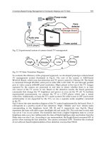
Fig. 12. Experimental system of camera-based TV management

wait
wait
X
X
High
Middle
Low
Sleep
X
X
X
wait
X
ON
wait
wait
X
X
X
High
Middle
Low
Sleep
X
X
X
XX

wait
X
ON

Fig. 13. TV State Transition Diagram
To evaluate the efficiency of the proposed approach, we developed prototype camera-based
TV management system illustrated in Fig.12. The core of the system is ARM-based
BEAGLE-Board, which runs face-detection and TV power control in Ubuntu OS. The board
is connected through RS-232C serial port to 42in NEC LCD V421 TV and through parallel
port to video camera (640x480 pixel resolution, 30fps) placed at the top of the TV. Images
captured by the camera are processed in real time to detect whether there is at least
one viewer of the TV screen or not. Based on the detection results, the board generates
commands that change the TV brightness and power or even set the TV off. To facilitate
experimental measurement, we connect the TV to a DVD player which runs a tested
video film. Additionally, to keep the TV’s audio system ON while screen is OFF (such mode
unfortunately is not supported by the TV), we use a separate audio amplifier connected
to the TV.
Fig.13 shows the state transition diagram of the TV control implemented by the board. Here, X
corresponds to a positive result of face detection; ‘High’, ‘Middle’ and ‘Low’ denote states
corresponding to the brightness levels 100, 50 and 0, respectively (see Fig.14); ‘Sleep’
represents the state with dark screen (backlight off) and audio ON. The wait time in each state
was set to 5 sec in our system. The transition time from a higher brightness state to a lower
brightness state was a few milliseconds; the time of High-brightness state reactivation from the
Sleep state was also 5 sec. According to our measurement, the Beagle-Board consumed 4W of
power when running the face detection. The camera consumed 0.5W. Therefore the overhead
of our software based implementation of face detection was less than 5Watt.

Energy Technology and Management

152

0
50
100
150
200
250
0 102030405060708090100
Brightness level
Power (W)
Low
Middle
High
0
50
100
150
200
250
0 102030405060708090100
Brightness level
Power (W)
Low
Middle
High

Fig. 14. The dependency of TV power consumption on brightness. The brightness levels
corresponding to selected power states are shown in red.
To evaluate energy efficiency of the proposed approach, we performed a number of tests,
each of each differed by the number of viewers, viewer behavior, the duration of time the
TV was viewed, the activities simultaneously done while watching TV, etc. (More details

about the tests can be found in [Moshnyaga 2011]). In all these tests, we measured the total
energy taken from the wall by all components of our system (TV, Beagle-board and camera)
and compared it to the energy consumed by TV in the motion-based screen-off mode, which
was set to the shortest (5min) period of inactivity.
The results reveal that the proposed energy management technology performs better then
Motion-Based Power Management (MBPM) when the TV users are either frequently
detracted from the screen by other activities or use it mainly for listening (as radio), not
watching. Even
with the shortest time setting, MBPM technique was unable to save energy
most of the time because of the viewer’s motion. In contrast, the energy saving achieved by
our method are high (up to 50-90%). Obviously, the savings depend on the user behavior.
If the viewer is not disrupted from TV by other activities, the proposed method adds 5 Watt
per hour overhead to the TV energy consumption. However, in comparison to TV power of
200W it is quite small. Moreover, whenever a 200W TV is left unwatched for longer than 1.2
min per hour, the proposed camera-based energy management works better than existing
motion-based user sensing. Fig.15 shows the screenshots of TV screen, camera readings on
PC display and the power meter: when there is a TV viewer, the screen is in High Brightness
mode (power: 206.4W); else the screen is dimmed and eventually enters sleep mode– bottom
picture (power: 5.2W).
Fig.16 exemplifies the TV power consumption during typical 2 hours long TV watching by
two users. The power bursts in the figure correspond to the screen activation when the
viewer returns his gaze to the screen. Notice, the MBPM takes around 200W all the time
independently of the viewer behavior. Even though the power savings achieved by our
CBPM system in comparison to MBPM on this test were not as impressive as on the other
tests there was quite large: 29%.

A Camera-Based Energy Management of Computer Displays and TV Sets

153

Fig. 15. Screenshots of TV and corresponding power consumption: when viewers looks at
screen, the screen is bright (power: 206.4W); else the screen is dimmed (power: 5.2W)

Energy Technology and Management

154
0
50
100
150
200
250
0 5 10 15 20 25 30 35 40 45 50 55 60 65 70 75 80 85 90 95 100 105 110 115 120
Time (min)
Power (W)
MBPM
0
50
100
150
200
250
0 5 10 15 20 25 30 35 40 45 50 55 60 65 70 75 80 85 90 95 100 105 110 115 120
Time (min)
Power (W)
MBPMMBPM

Fig. 16. A profile of power consumed by the proposed camera based power management
(CPBM) system in comparison to motion based power management (MBPM) during 2 hours
long typical TV watching.
4. Conclusion
In this paper we presented a new technology for energy management in computer display
and TV set based on camera-based viewer monitoring. For the PC display, we track eyes of
the user, while for the TV set faces of its viewers, keeping the screen active only when
someone looks at it. Experiments showed that the technology saves more energy than
existing schemes monitoring viewers behavior in real-time with high accuracy. The current
implementation of PC display energy management in FPGA consumes only 1W of power
while implementation of camera-based TV energy management in low-power embedded
system (Beagle-Board) takes only 5W.
A possible solution to reduce power overhead could be in designing a custom LSI chip for
viewer detection, similarly to those implemented in photo camera. This will push the energy
overhead to the mW level.
The research presented here is a work in progress and the list of things to improve it is long.
In the current work on PC energy management, we restricted ourselves to a simple case of a
singular user. However, when talking about the user-gaze monitoring in general, some
critical issues arise. For instance, how to handle more than PC user? The main PC user
might not look at screen while the others do. Concerning this point, we believe that a
feasible solution is to keep the display active while there is someone looking at the screen.
The TV viewer monitoring also has several challenging issues. First, the viewers can be
positioned quite far from the TV set. Second, the viewers can watch TV when laying on a
bed or a sofa, so the viewer’s face can rotate on a large angle. Third, the face illumination
condition may change from a very bright to a complete darkness. In these conditions, the
correct real-time face monitoring with low-energy overhead becomes really difficult. Our
future study will cover the use of IR-camera, impact of face orientation, face color and other
issues.
5. Acknowledgment
The work was sponsored by The Ministry of Education, Culture, Sports, Science and

Technology of Japan under Regional Innovation Cluster Program (Global Type, 2nd Stage)
and Grant-in-Aid for Scientific Research (C) No.21500063.

A Camera-Based Energy Management of Computer Displays and TV Sets

155
6. References
ACPI: Advanced Configuration and Power Interface Specification, Rev.3.0, Sept.2004,
o/spec.htm
BeagleBoard: System Reference Manual, Rev.4, available from
Baluja, S., Pomerlau, D. (1994) Non intrusivegaze tracking using artificial neural networks,
Technical report CMU-CS-94-102.
Chang N., Choi I., and Shim H. (2004) DLS: dynamic backlight luminance scaling of liquid
crystal display, IEEE Trans. VLSI Systems, vol.12, no.8, pp.837-846.
Cheng W C. , Pedram M. (2004) Power minimization in a Backlight TFT-LCD display by
concurrent brightness and contrast scaling, Proceedings of the Design Automation
and Test in Europe, Vol. 1, pp. 16-20.
Choi L., Shim H., Chang N. (2002) Low power color TFT LCD display for hand-held
embedded systems, Proceedings of International Symposium on Low-Power
Electronics and Design, pp.112-117.
Coughlan S., (2006) Do flat-screen TVs eat more energy? BBC News, 7 Dec.2006

Dai X. and Raychandran K., (2003) Computer screen power management through detection
of user presence, US Patent 6650322, Nov.18.
Douxchamps D., Campbell N., Robust real time face tracking for the analysis of human
behavior, in Machine Learning for multimodal Interaction, LNCS 4892, 1-10, 2002.
Elias E. W. A., Dekoninck E. A., Culley S. J., (2007) The Potential for Domestic Energy
Savings through Assessing User Behaviour and Changes in Design, 5
th

International Symposium on Environmentally Conscious Design and Inverse
Manufacturing, Tokyo, Japan, 2007.
Fujitsu-Siemens (2006) Energy savings with personal computers, from itsu-
siemens.nl/aboutus/sor/energy_saving/prof_desk_prod.html
Flinn J., and Satyanarayanan S. (1999) Energy-aware adaptation for mobile applications,
Proceedings of the Symposium on Operating Systems Principles, pp.48-63
Gatti F., Acquaviva A., Benini L., Ricco B. (2002) Low-power control techniques for TFT LCD
displays. Proceedings of the International Conference on Compilers, Architecture
and Synthesis for Embedded Systems, pp.218-224
Hewlett-Packard Co. (2006), Global Citizenship Report”, available from www.hp.com/
hpinfo/globalcitizenship/gcreport/pdf/hp2006gcreport_lowres.pdf
Generation M2: Media in the lives of 8-18 years old. A Kaiser Family Foundation Study,
(2010, June). Henry J. Kaiser Family Foundation, Menlo Park, California, (79 pages)
Gram-Hansen K. (2003), Domestic electricity consumption - consumers and appliances,
Nordic Conference on Environmental Social Sciences.
Iranli A., Lee W., Pedram M., (2006)“HVS-Aware Dynamic Backlight Scaling in TFT-LCDs,”
IEEE Trans. on Very Large-Scale Integration Systems, Vol. 14, No. 10, pp. 1103-1110.
Ji Q., Zhu Z. (2002) Eye and gaze tracking for interactive graphic display. Proceedings of the
ACM Int. Symposium on Smart Graphics.
Kawato S., and Ohya J. (2000) Two-step approach for real-time eye-tracking with a new
filtering technique. IEEE Int. Conf. of Systems, Man & Cybernetics, 1366-1371.
Kawato S., Tetsutani N., Osaka K. (2005) Scale-adaptive face detection and tracking in real
time with SSR filters and support vector machine, IEICE Trans. Information &
Systems, E88-D, (12) 2857-2863.
Lee C.G. and Moshnyaga V.G. (2011) TV Energy management by Camera-Based User
Monitoring, Proceedings of the IEEE International Symposium on Circuits and Systems.

Energy Technology and Management

156

Mahesri A., Vardhan V. , (2005) Power Consumption Breakdown on a Modern Laptop,
Proceedings of the Power Aware Computer Systems, LNCS, vol.3471,pp.165-180,2005.
Moshnyaga V.G., Morikawa E. (2005) LCD Display Energy Reduction by User Monitoring,
Proc. Int. Conf. on Computer Design, pp.94-97.
Moshnyaga V.G., Hashimoto K., Suetsugu T., Higashi S. (2009) A hardware implementation
of the user-centric display energy management, LNCS 5953, Springer, 56-65.
Nielsen Media Research Inc., (2009) Television Audience 2009. The Nielsen Company
Nordman, Bruce, Mary Ann Piette, and Kris Kinney. 1996. Measured Energy Savings and
Performance ofPower-Managed Personal Computers and Monitors. LBL-38057. Lawrence
Berkeley National Lab., available at
Nordman, Bruce, Mary Ann Piette, Kris Kinney, and Carrie Webber. 1997. User Guide to
Power Management for PCs and Monitors. LBNL-39466. Lawrence Berkeley National
Lab., available at:
Ohno T., Mukawa N., Kawato S. (2003) Just blink your eyes: a head-free gaze tracking
system. Proceedings of the CHI 2003, 950-951.
Open CV: Open Computer Vision Library, available at

Park, W.I., (1999) Power saving in a portable computer, EU Patent, EP0949557, 1999
Park, R, Kim, J. (2005) Real-time facial and eye gaze tracking system, IEICE Transaction on
Information & Systems., E88-D (6), 1231-1238.
Pasricha S. Luthra M., Mohapatra S., Dutt N., and Venkatasubramanian N. Dynamic
backlight adaptation for low-power handheld devices, IEEE Design and Test
Magazine, Sept/Oct. 2004, pp. 398-405.
Pattanai K.S.N., Tumblin J.E., Yee H., and Greenberg D.P. (2000) Time dependent visual
adaptation for realistic image display”, Proceedings of the SIGGRAPH, pp.47-54.
Robertson J. , Homan G.K., Mahajan A., et al, (2002) Energy use and power levels in new
monitors and personal computers”, LBNL-48581, UC Berkeley, July 2002
Plasma TV: Performance Test Results - Power consumption Tests (2006),

Sharp Microelectronics of the Americas, (2002), Display Modes :Transmissive/Reflective/

Transflective, available from:
displays/AppRefGuide/DisplayModes.htm
Shim H., Chang N., and Pedram M. (2004 Sept/Oct) A backlight power management
framework for the battery-operated multi-media systems. IEEE Design and Test
Magazine, pp. 388-396.
Theocharides T., Link G., Vijakrishnan N., Irwin M.J., Wolf W. (2004) Embedded Hardware
Face Detection, 17th IEEE Int. Conf. VLSI Design, pp.133-138.
Tumblin J.E. , Hodgins J.K. , and Guenter B.K. (1999) Two methods for display of high
contrast images. ACM Transactions on Graphics, Vol.18, no.1, pp. 56-94, Jan.1999.
TV Power Consumption: Is There a Problem? (and Can LCD TVs Help?) LCD TV
Association, 2008, available from www.LCDTVAssociation.ORG
Television & Health,
Viola P. and Jones M. (2001) Rapid object detection using a boosted cascade of simple
features. Proceedings of the IEEE International Conference on Computer Vision and
Pattern Recognition.
Yamamoto S. and Moshnyaga V.G. (2009) Algorithm optimizations for low-complexity eye
tracking. Proceedings of the IEEE International Conference on Systems, Man and
Cybernetics, 18-22.
8
Enhancement of Power System State Estimation
Bei Gou
1
and Weibiao Wu
2

1
Department of Electrical and Computer Engineering, North Dakota State University
2
Department of Statistics, University of Chicago
USA

1. Introduction

Power Utility companies use the state estimator to provide system operating status to the
operators of their control center to allow them to manage and to take appropriate measures
to prevent the loss of electricity. The unavailability of state estimation solution may cause
the occurrence of cascading failures or blackouts in local and/or regional areas for
considerable time periods, if disturbance occurs during the period of unavailability and thus
can not be closely monitored. The robustness and reliability of state estimation is a critical
issue and concern of power utilities.
The Weighted Least Square (WLS) method is the commonly used state estimation
methodological approach in power industry. If one or more gross errors are contained in the
measurements the WLS state estimator may not reach a solution and diverge. A well-known
example when the WLS did not converge due to the existence of a topology error was a
indirect contributing factor to the August Blackout in Northeastern U.S. in 2003. According
to the President’s Task Force the operator could not determine the status of the system
because of a computer program ‘glitch’. This ‘glitch’ was a failure of the WLS method to
converge and give a solution to the State Estimation. Task Force comments noted the
‘unacceptability’ of such computer program errors when the economic impact of the
consequential blackout was so dramatic. The economic damage of the 2003 blackout was
reported to be in excess of $10 Billion dollars.
The following figure shows the convergence property of WLS state estimation. This figure
was obtained on IEEE-118 bus system. WLS state estimation has been simulated on 5000
different patterns of load levels for IEEE 118-bus system. It is clear to see that WLS state
estimation will be completely unfunctional after the load level reaches a specific amount.
Details of this simulation will be explained later in the chapter.
The need to detect the gross errors is a critical and challenging issue for WLS state
estimation. Many researchers have tried to develop algorithms to detect gross errors for
WSL state estimation without dramatic success. Most of the detection techniques proposed
so far are based on a solution of WLS state estimation. The dilemma is that detecting gross
errors requires a solution of state estimation under the presence of gross errors that solution

may not occur.
Topology errors are classified in two categories: branch status errors and substation
configuration errors (Abur and A.G. Exposito, 2004). The analysis of conditions upon which
topology errors can be detected was presented in (K. A. Clements and A. Simoes-Costa, 1988

Energy Technology and Management

158
and F. F. Wu and E. H. E. Liu, 1989). A geometric interpretation of the measurement
residuals for topology errors identification was provided in (K. A. Clements and A. Simoes-
Costa, 1988) which also proposed a systematic analysis of the normalized residuals to detect
the bus configuration errors. Ref. (F. F. Wu and E. H. E. Liu, 1989) presented the effect of
measurement equations when including topology errors and proposed a method to detect
the topology errors by residual analysis. A method based on the number of measurements
labeled as bad data was proposed in (H. J. Koglin et al 1986, H. H. J. Koglin and H. T.
Neisius, 1990, and H. J. Koglin and H. T. Neisius, 1993). A robust Huber estimator based on
an approximate decoupled model was proposed in (L. Mili et al, 1999) as a means of pre-
checking the assumed system topology. Effects of topology errors can be considered
explicitly by representing the circuit breakers in terms of the real and reactive power flows
(Monticelli and A. Garcia, 1991, Monticelli, 1993, and Monticelli, 1993). Observability of
breaker flows and cases of undetectable breaker status errors are identifies by the WLAV
estimator (Abur et al, 1995). LAV was also used to detect the topology errors in (H. Singh
and F. L. Alvarado, 1995). A generalized state estimation was proposed to identify topology
errors in (E. M. Lourenco, et al, 2004, and O. Alsac, et al, 1998).

6400 6600 6800 7000 7200 7400 7600 7800 8000
0
0.2
0.4
0.6

0.8
1
Load Levels (MW)
Frequency of Convergence
Comparison of Convergence between WLS and the Proposed Approach
WLS
Proposed Approach

Fig. 1. Divergence rate of WLS state estimator for different load levels in IEEE 118 bus test
system.
The newly developed disruptive state estimator is based on a totally different philosophy
that does not require a solution of state estimation. As the divergence of the WLS state
estimation occurs far too frequently it is to the new approach’s merit that a solution of the
system is not needed. This new innovative approach also is able to provide a reasonable
state estimation solution under any circumstance.
2. Proposed bad data processing algorithm
For a transmission line, if the voltage at one end and parameters of the line are known, then
the voltage of the other end can be uniquely calculated from the power flow on this line. The

Enhancement of Power System State Estimation

159
idea can be applied to the entire system: if a tree formed by branch flow measurements and
the root voltage is known, then the voltages of the whole system can be uniquely calculated
(P. Bonanomi and G. Gramberg, 1983). The idea is re-studied in this paper.
The proposed algorithms in this paper are totally different from the one in (P. Bonanomi
and G. Gramberg, 1983):
1. The tree defined above in (P. Bonanomi and G. Gramberg, 1983) does not always exist and
the authors of (P. Bonanomi and G. Gramberg, 1983) did not solve this problem (see
discussion in (P. Bonanomi and G. Gramberg, 1983)). This paper solves this problem by

introducing an Extended Solving Tree. With suitable adjustment, the PI’s proposed
algorithms of observability analysis (Bei Gou, 2007, Bei Gou and Ali Abur, 2000, Bei Gou
and Ali Abur, 2001, Bei Gou, 2006) can be used to find an extended solving tree and the
redundant measurements for all the measurements in the extended solving tree;
2. The bad data detection method is totally different: (P. Bonanomi and G. Gramberg,
1983) made use of KCL and KVL laws and this paper uses the residuals of redundant
measurements which is clearer and more efficient in bad data detection;
3. This paper proposes an non-iterative robust state estimation which is equivalent to the
weighted least square, and therefore the best estimates of the states can always be
obtained under any circumstances.
2.1 Extended solving tree
If there does not exist a tree of measurements to connect all the buses in an island (sub-
network), then this island can be processed individually and solved by using WLS. Then the
extended solving tree is defined to be a tree that contains not only transmission lines
assigned by measurements but also islands whose sizes are minimized.
In the following context, we will still use solving tree for the description, but it should be
note that the description is also true for the extended solving tree.
Definitions
Before the description, we give the following definitions:
• Bus Distance: the Bus Distance between buses i and
j is defined as
22
||(||||)()
ij i j i j i j
dVV V V=−= − +θ−θ
.
• Parent Bus: bus A is called a parent bus of bus B when bus B can be directly solved from
bus A. A bus can only have one parent bus in a solving tree.
• Children Buses: Bus A is called a children bus of bus B when bus A can be directly solved
from bus B. A bus can have multiple children buses in a solving tree.

• Ancestor Buses: ancestor buses of bus A are defined to be all the buses solved before bus
A. Ancestor buses also forms an island.
• Descendent Buses: descendent buses of bus A are defined to be all the buses that can be
solved only after bus A is solved. Descendent buses also forms an island.
• Recovered Power Flows of a solving tree: are defined to be the power flows and power
injections that are calculated from the solution of the solving tree.
2.2 Error propagation

For a solving tree, it is obvious to see that an error present in any of the measurement in the
solving tree will be propagated to its descendent buses. We will show that the following
Theorem is true.

Energy Technology and Management

160
Lemma 1: For a given set of redundant measurements, if this set of measurements is perfect,
then the solutions of any possible solving trees are identical, and equal to the one when all
the measurements are used.
Theorem 2: If a bad data appears in a measurement of a solving tree, then all the recovered
power flows corresponding to the redundant measurements of this measurement contain a
gross error.
Proof:
Let us assume all the measurements are perfect except a gross error in a flow measurement
km
S (see Fig. 1 for the explanation) that is included in a solving tree l .
km
S is a measurement
connecting two islands: one is formed by the ancestor buses of
km
S and the other is formed

by the descendent buses of
km
S
. Suppose a gross error appear in
km
S
. So the voltage
m
V

contains an error. Assume one of the redundant measurements of
r
S is recovered and equal
to
r
S

. Now we need to prove that
r
S

is different from
r
S which is perfect.
We assume that
r
S

equals
r

S

Now if we form a new solving tree
1
l by including
r
S in l and discarding
km
S . The new
solving tree forms a tree and can still solve the whole system. Since
rr
SS=

, so the solving
tree
1
l
obtains the same solution as that of l . That means that voltage
m
V
at bus m solved
from
1
l is the same as the voltage solved from the solving tree l . And
m
V contains an error
due to the error appearing in
km
S in l .
However, since all the measurements in the solving tree

1
l
are perfect, Lemma 1 shows that
we should obtain an exact solution. That means that the voltage at bus
m
should be
accurate. We reach a contradiction! Therefore, our assumption is wrong.
r
S

does not equal
to
r
S
. We conclude the proof. ■
Remarks:
1. Theorem 2 implies that all the voltages at the descendent buses of a measurement
km
S
are pushed in-group to a wrong place by the error in
km
S ;
2. Theorem 2 implies that any error including bad data in a measurement of the solving
tree, topology error or parameter error in a line of the solving tree, will cause obvious
errors in the residuals of the redundant measurements of that measurement.
Examples for theorem 2
A) Gross error in measurement
Let us look at an example. In this example, we introduced a gross error (change the sign) to the
real power measurement on branch 4-7. In Fig. 2, we can see that some of the voltages showed
by ‘+’ and ‘O’ are overlapped, while other voltages showed by ‘+’ are moved down, which

indicates the approximately same error is attached to all the descendent buses of bus 4.
Detection: The recovered power flows, which correspond to the redundant measurements of
this measurement, should have big deviations from the redundant measurements. This
feature can be used to detect errors in the measurements.
B) Error in branch parameter
In the same system and measurement configuration, we added an error in the parameter of
branch 7-9. The comparison of voltages with and without parameter error is shown in Fig. 3.
Detection: Assume the measurement be perfect on the branch 7-9 that has a parameter error.
If the measurement on branch 7-9 is replaced by one of its redundant measurements to form


Enhancement of Power System State Estimation

161


Fig. 2. Explanation of the proof




Fig. 3. Comparison of Voltages with and without Errors
km
S
r
S
r
S

Solving

Tree
l
Bus m
Solving
Tree
1
l
Ancestor Island of
branch k-m
Descendent Island
of Branch k-m
Bus
k

Energy Technology and Management

162
a new solving tree, then the recovered power flow of branch 7-9, calculated from the
solution of the new solving tree, should be equal to the measurement on branch 7-9. This
feature can be used to detect the branch parameter errors.


Fig. 4. Comparison of Voltages with and without Parameter Error
C) Topology error
Furthermore, we added a topology error on branch 13-14 that is wrongly considered to be
closed while it is actually open. The comparison of voltage with and without topology error
shows that only the voltages at the descendent buses of branch 13-14 have errors, which is
shown in Fig. 4.
Detection: Assume the injection measurement at bus 14 is error-free. Then the assigned flow
measurement on branch 12-13. The voltages between these two buses have very close

voltages showing in Fig. 4. This feature can be used to detect the topology error.
Bad data detection
Once the recovered measurements are obtained from the solution of a solving tree, we are
able to detect the bad data. The main idea to detect the bad data is to use the redundant
measurements. Here we assume that there are no critical measurements and critical pairs.
For a solving tree, every measurement (real flow or reactive flow) has at least two redundant
measurements that connect the ancestor island and descendent island of this measurement.
The residuals of these redundant measurements (the difference between the redundant
measurements and their recovered power flows) can be directly used to detect the bad data.
Hypothesis Testing Technique (L. Mili, et al 1984) is used to detect the bad data.
The multiple interacting and confirming bad data can be detected by the proposed bad data
detection algorithm. We do not need to study it separately.
Critical measurement and critical pairs
Comparing the maximum historical bus distance with the bus distance calculated from the
solving tree is possibly able to detect the bad data in the measurements.

Enhancement of Power System State Estimation

163

Fig. 5. Comparison of Voltage with and without Topology Error
3. A numerical test example
IEEE 14 bus system is used to test the proposed robust state estimator. A solving tree l is
found which is given in Figures 1 and 2.
Three gross errors are added: 1) a topology error on branch 4-7: an open breaker on branch
4-7 is wrongly considered to be closed; 2) a sign change on real power measurement
79
P
;
and 3) a sign change on reactive power measurement
9,10
Q . The redundant measurements
are flows on branches 2-4, 4-2, 4-5, 5-4, 4-9, 9-4, 6-11, 11-6, 6-12, 12-6, 6-13, 13-6, 9-7; injections
at buses
A solution is obtained from the solving tree and power flows are recovered. Comparing the
residuals of original measurements and the recovered power flows, we found the following
measurements having biggest residuals: real and reactive power flow measurements on
branches: 2-4, 4-2, 4-5, 5-4, 4-9, 9-4, 6-11, 11-6, 6-12, 12-6, 6-13, 13-6; and real power flow
measurement
97
P (
79
P is a measurement in the solving tree).

Big residuals on branches 2-4, 5-4, 6-11, 6-12, 6-13 show that there must be a gross error in
the measurement (injection at bus 3) that is assigned to branch 3-4. We removed the injection
measurement at bus 3, and add the measurement on branch 2-4 (
24
P and
24
Q ) to form a
new solving tree
1
l
.
Solve the system by using
1
l and calculate the residuals of original redundant
measurements and their recovered power flows. We found the following branches having
big residuals: real and reactive power flow measurements on branches 4-9, 6-11, 6-12, 6-13,
and the real power flow
97
P on branch 9-7. It is obvious that those branches indicate a gross
error in the measurement on branch 7-9.
We removed
79
P
,
79
Q
and add
97
P
,

97
Q
on the branch 7-9 to form a new solving tree
2
l
.
Solve the system and calculate the residuals, we found
11,6
Q and
10,9
Q have big residuals.
Their corresponding measurement in
2
l is
9,10
P and
9,10
Q . We replaced them with their

Descendent Buses
(13 & 12) of Branch
13-14


Energy Technology and Management

164
redundant measurements
6,11
P and

6,11
Q to form a new solving tree
3
l . The residuals from
the solution of solving tree
3
l are all very small.
Then we concert all the redundant measurements to the solving tree, for example, branch
flows on 6-12 and 6-13 were converted to measurements on 1-2, injection at bus 10 was
converted to flows on 9-10, voltage magnitude measurement at bus 14 was converted to bus
1, etc. After all the redundant measurements were converted, we calculated the voltages at
all the buses by using the updated solving tree
3
l and reached the best estimates of IEEE 14-
bus system (see Table I). White noises having zero mean and 0.001 standard deviation were
added to all the measurements.

Bus
Solution from Solving
Tree
||V
θ
1
1.0610 0.0
2
1.0459 -4.980
3
1.0109 -12.710
4
1.0193 -10.320

5
1.0211 -8.770
6
1.0708 -14.210
7
1.0624 -13.370
8
1.0903 -13.370
9
1.0568 -14.950
10
1.0514 -15.110
11
1.0570 -14.800
12
1.0549 -15.080
13
1.0502 -15.160
14
1.0361 -16.030
Table 1. Estimates of system states from the solving tree
4. Simulation results
The comparison between WLS and our new approach has been performed on IEEE 118 bus
system. Three test scenarios that include two random bad data, two random interacting and
conforming bad data, and two random topology errors, have been examined. Identical sets
of measurements were tested for both approaches. Under light load levels, the new
approach is several percent better [99.7%] than the WLS method [97%] in detecting topology
errors. Under heavy loads where the WLS method frequently fails to reach a solution and
the new approach is very superior.

Enhancement of Power System State Estimation

165
To validate the new approach we also examined the new approach on a real power system
with 5145 buses. A clear delineation between the two methods at a certain load level is
apparent, which shows the similar characteristics as IEEE-118 bus system.
A) Comparison-local redundancy method vs. WLS
In this comparison random two bad data were simulated on IEEE-118 bus system with 5000
different load levels.
Random bad data

Method # of Divergence # of Bad Data Detected
New
Approach
0% 91.2%
WLS 61.5% 36.2%
Table 2. Comparison of convergence of the proposed algorithm with the WLS state
estimation
The simulation results are displayed in above table, which shows that the new approach
always converges and is able to detect the bad data for most of the cases. Fig. 5 shows the
comparison of bad data detection between WLS and the new approach. It is obvious to see
that the new approach is much more robust than WLS for all different load levels.

3000 4000 5000 6000 7000 8000 9000 10000 11000
0
0.2
0.4
0.6
0.8
1

Load Level (MW)
Frequency of finding bad data
Comparision between WLS and the New Approach for 2 random bad data

Fig. 6. Comparison of bad data detection between the new approach and WLS

Energy Technology and Management

166
Interacting and conforming bad data
It is known that WLS state estimation has difficulty in detecting the interacting and
conforming bad data. This simulation is aimed to test the detection capability of the new
approach and its comparison to WLS state estimation. The following table shows the results
of comparison. The comparison indicates that the new approach is much more robust than
the traditional WLS stat estimation.

Method # of Divergence # of Bad Data Detected
New
Approach
0% 89.8%
WLS 50.2% 38.1%
Table 3. Comparison of convergence of the proposed algorithm with the WLS state
estimation
Fig. 6 shows the comparison of multiple interacting and conforming bad data detection
between the new approach and WLS state estimation. The comparison implies that the new
approach is much more robust than traditional WLS state estimation and has higher
percentage of error detection in light load levels.

3000 4000 5000 6000 7000 8000 9000 10000 11000
0

0.1
0.2
0.3
0.4
0.5
0.6
0.7
0.8
0.9
1
Load Level (MW)
Frequency of finding bad data
Comparision between WLS and the New Approach for 2 intacting & conforming bad data



Fig. 7. Comparison of interacting and conforming bad data detection between the new
approach and WLS

Enhancement of Power System State Estimation

167
Topology errors
Topology error is currently the biggest concern of power system operators, especially after
the occurrence of North American Blackout in August 2003. Topology errors are severe
gross errors, which can make the state estimation fail to converge. This simulation is to test
the capability of the new approach in detecting topology errors. The following table shows
the comparison of topology error detection between traditional WLS state estimation and
the new approach. It is obvious to see that the new approach is much more robust.
Fig. 7 shows the comparison of topology error detection between traditional WLS state

estimation and the new approach, under different load levels. The results indicates that WLS
state estimation has good detection capability only when the system load is light; the topology
error detection capability of WLS drops very fast if the load level reaches a certain amount. On
the other hand, the new approach has a very stable capability of topology error detection. It is
obvious that the new approach is much more robust than traditional WLS state estimation.

Method # of Divergence # of Bad Data Detected
New
Approach
0% 99.5%
WLS 53% 46.7%
Table 4. Comparison of convergence of the proposed algorithm with the WLS state
estimation

3000 4000 5000 6000 7000 8000 9000 10000 11000
0
0.1
0.2
0.3
0.4
0.5
0.6
0.7
0.8
0.9
1
Load Level (MW)
Frequency of finding topological errors
Comparision between WLS and the New Approach for 2 topological errors

Fig. 8. Comparison of topology error detection between the new approach and WLS

Energy Technology and Management

168
Comparison on a real system with 5145 buses
A real power system with 5145 buses was used to test the new approach. Because from the
above tests we found that the divergence of WLS state estimation is the main reason of non-
robustness of WLS state estimation, we only compare the convergence ability of the new
approach and WLS state estimation on this real system. In this test 6658 branch flow
measurements, 1000 injection measurements and 500 voltage measurements are used. 500
sets of measurements were generated by randomly selecting the locations of all the
measurements. Here are the results of this test.
The new approach
The new approach was able to get convergent and accurate solutions for these 500 sets of
measurements.
WLS state estimation
WLS state estimation failed to get solutions for 169 sets of measurements, and converged to
unacceptable solution for 165 sets of measurements, and only converged to accurate
solutions for 165 sets of measurements.

4000 5000 6000 7000 8000 9000 10000 11000
0.84
0.86
0.88
0.9
0.92
0.94
0.96
Load Level (MW)

Minimum Voltage Magnitude (p.u.)
Minimum Voltage v.s. Load Level



Fig. 9. Minimum voltage magnitudes for 500 sets of measurements.
5. Conclusion
Since topology error is currently the main concern of power system operators, it is very
important to develop a robust state estimation that is robust and not dependent on a solution
of state estimation. A new approach of topology error detection has been proposed in this
paper. The newly developed disruptive state estimator is based on a totally different
philosophy that does not require a solution of state estimation. As the divergence of the WLS

Enhancement of Power System State Estimation

169
state estimation occurs far too frequently it is to the new approach’s merit that a solution of the
system is not needed. Various tests have been conducted on IEEE 118-bus system and a real
system with 5145 buses. The results show that the new approach is much more robust than
traditional WLS state estimation, and it is ready to be applied in power industry.
6. References
Abur and A.G. Exposito, (2004). Power System State Estimation: Theory and
Implementation, Marcel Dekker, ISBN 0824755707
K. A. Clements and A. Simoes-Costa, (1988). Detection and Identification of Topology Errors
in Electric Power Systems, IEEE Trans. on Power Systems, Vol. 3, No. 4, pp. 1748-
1753
F. F. Wu and E. H. E. Liu, (1989). Detection of Topology Errors by State Estimation, IEEE
Trans. on Power Systems, Vol. 4, pp. 176-183
H. J. Koglin, D. Oeding and K. D. Schmitt, (1986). Identification of Topology Errors in State
Estimation, IEE International Conference on Power System Monitoring and

Control,
Durham, pp. 140-144 H. H. J. Koglin and H. T. Neisius, (1990). Treatment of Topology Errors
in Substations, Proc. 10
th
Power Systems Computation Conference, Butterworth,
Graz, pp. 1045-1053
H. J. Koglin and H. T. Neisius, (1993). A Topology Processor Based on State Estimation,
Proceedings of the 11
th
Power Systems Computation Conference, pp. 633-638,
Avignon
L. Mili, G. Steeno, F. Dobraca, and D. French, (1999). A Robust Estimation Method for
Topology Error Identification, IEEE Transactions on Power Systems, Vol. 14, No. 4,
pp. 1469-1476
Monticelli and A. Garcia, (1991). Modeling Zero Impedance Branches in Power System State
Estimation, IEEE Trans. on Power Systems, Vol. 6, No. 4, pp. 1561-1570
Monticelli, (1993). Modeling Circuit Breakers in Weighted Least Square State Estimation,
IEEE Trans. on Power Systems, Vol. 8, No. 3, pp. 1143-1149
Monticelli, (1993). The Impact of Modeling Short Circuit Branches in State Estimation, IEEE
Trans. on Power Systems, Vol. 8, No. 1, pp. 364-370
Abur, H. Kim and M. Celik, (1995). Identifying the Unknown Circuit Breaker Status in
Power Networks, IEEE Trans. on Power Systems, Vol. 10, No. 4, pp. 2029-2037
H. Singh and F. L. Alvarado, (1995). Network Topology Determination Using Least
Absolute Value State Estimation, IEEE Trans. on Power Systems, Vol. 10, No. 3, pp.
1159-1165
E. M. Lourenco, A. S. Costa and K. S. Clements, (2004). Bayesian-based hypothesis testing
for topology error identification in generalized state estimation, IEEE Trans. on
Power Systems, Vol. 9, No. 2, pp. 1206-1215
O. Alsac, N. Vempati, B. Stott and A. Monticelli, (1998). Generalized state estimation, IEEE
Trans. on Power Systems, Vol. 13, No. 3, pp. 1069-1075

P. Bonanomi and G. Gramberg, (1983). Power System Data Validation and State Calculation
by Network Search Techniques, IEEE Trans. on Power Apparatus and Systems,
Vol. PAS-102m No. 1, pp. 238-249
Bei Gou, (2007). Observability Analysis for State Estimation Using Hactel's Augmented
Matrix Method, Electric Power Systems Research, Vol. 77, No. 7, pp: 865-875

Energy Technology and Management

170
Bei Gou and Ali Abur, (2000). A direct numerical method for observability analysis, IEEE
Trans. on Power Systems, Vol. 15, No. 2, pp. 625-630
Bei Gou and Ali Abur, (2001). An improved measurement placement algorithm for network
observability, IEEE Trans. on Power Systems, Vol. 16, No. 4, pp. 819-824
Bei Gou, (2006). Jacobian matrix-based observability analysis for state estimation, IEEE
Trans. on Power Systems, Vol. 21, No. 1, pp. 348-356
L. Mili, Th. van Cutsem, and M. Ribbens-Pavella, (1984). Hypothesis Testing Identification: a
New Method for Bad Data Analysis in Power System State Estimation, IEEE
Transactions on Power Apparatus and Systems, Vol. PAS-104, No. 11, pp. 3239-
3252