Laser Pulse Phenomena and Applications Part 8 ppt

Time-gated Single Photon Counting Lock-in Detection at 1550 nm Wavelength

201
0 20000 40000 60000 80000 100000
0
20
40
60
80


162mV
184mV
Lock-in Signal ( µV)
Photon Counts (cps)
150 160 170 180 190 200
10
100
1000
10000
100000
1000000
1E7
0.0
0.3
0.6
0.9
1.2
1.5
1.8
counts

Photon counts
Threshold Level (mV)
lock-in output ( µV)
lock-in output
(a)
(b)

Fig. 8. (a) Dark count and its lock-in measurements vs discriminate threshold. (b) Single
photon lock-in outputs vs threshold with different photon counts. The single photon lock-in
outputs vs photon counts for threshold being 162 mV and 184 mV, respectively.
The frequency spectrum of the monitor out of lock-in amplifier is shown in Fig. 7 (a). Here,
the mean photon number is 100 kcps and the SR400 threshold is 184mV. Note that the single
photon modulation signal at the place of frequency 100 kHz. As the dark counts of the
SPAD follow Poisson statistics, i.e., dominating shot noise with white noise spectral density,
we found the uniform distribution of the background noise. The effect of Flicker noise (l/f)
noise on the accuracy of measurements can be ignored. At lower threshold, the (l/f) noise
may become dominant, so we choose the 100 kHz for single photon modulation, due to the
higher noise in the low-frequency region.
As shown in Fig. 7 (b), when we change the level discrimination from 184 mV to 162 mV, it
is found that the dark counts increase quickly which cover 4 orders of magnitude where the
weak photon signals will be immerged in the case at lower threshold. The limit to detection
efficiency is primarily device saturation from dark counts.
In Fig. 7 (b), we show the single photon lock-in output corresponding to different mean
photon counts, 10 kcps, 25 kcps, 50 kcps and 100 kcps, respectively. The data are obtained
by first setting the discriminate voltage, and measuring the mean photon counts and lock-in
output respectively. The traces show the discriminate threshold can be optimized at 162 mV
where the lock-in has the maximum output.
Accordingly, we have measured the lock-in output with the lock-in integrated time 100 ms,

and the equivalent noise bandwidth for bandpass filter Δf =1 Hz. It is interesting to note that
the lock-in output increase only 4 times from 184 mV to 162 mV in Fig. 8 (a).
The demodulated signals versus photon counts for discriminate threshold being 162 mV
and 184 mV are shown in Fig. 8 (b). The two curves show that the intensity of single photon
lock-in signals are increasing linearly as the photon counts increased. The slope for the fitted
line is 1.24 μV/kcps at 184 mV threshold, and 2.32 μV/kcps at 162 mV, respectively. It is
shown that the detected efficiency with single photon lock-in at 162 mV is 1.87 times bigger
than that of the photon counting method at 184 mV.
We have demonstrated our measurement system in TGSPC experiment for a 3m-length
displacement between the two retroreflectors. The backscattered photons reach to the
InGaAs single photon detectors through a fiber optical circulator, as shown in Fig. 9. With
the 162 mV optimal threshold, the single photon lock-in for TGSPC experiment is shown as
Fig. 9, where the backscattered signal is presented as a function of length. Here it is found
Laser Pulse Phenomena and Applications

202
that the dark count and the photon shot noise are restrained, and clearly the conventional
photon counting is dogged by a high dark count rate at this low threshold.

Fig. 9. The TGSPC measurement by using single photons lock-in with the optimal threshold
162 mV.
4. Conclusion and outlook
The single photon detection for TGSPC which has some features of broad dynamic range,
fast response time and high spatial resolution, remove the effect of the response relaxation
properties of other photoelectric device. We present a photon counting lock-in method to
improve the SNR of TGSPC. It is shown that photon counts lock-in technology can eliminate
the effect of quantum fluctuation and improve the SNR. In addition, we demonstrate
experimentally to provide high detection efficiency for the SPAD by using the single photon
lock-in and the optimal discriminate determination. It is shown that the background noise
could be obviously depressed compared to that of the conventional single photon counting.

The novel method of photon-counting lock-in reduces illumination noise, detector dark
count noise, can suppress background, and importantly, enhance the detection efficiency of
single-photon detector.
The conclusions drawn give further encouragement to the possibility of using such ultra
sensitive detection system in very weak light measurement occasions (Alfonso & Ockman,
1968; Carlsson & Liljeborg, 1998). This high SNR measurement for TGSPC could improve
the dynamic range and time resolution effectively, and have the possibility of being applied
to single-photon sensing, quantum imaging and time of flight.
5. Acknowledgments
The project sponsored by the 863 Program (2009AA01Z319), 973 Program
(Nos.2006CB921603, 2006CB921102 and 2010CB923103), Natural Science Foundation of
Displacement (meter)
Lock-in output (μV)
Time-gated Single Photon Counting Lock-in Detection at 1550 nm Wavelength

203
China (Nos. 10674086 and 10934004), NSFC Project for Excellent Research Team (Grant No.
60821004), TSTIT and TYMIT of Shanxi province, and Shanxi Province Foundation for
Returned Scholars.
6. References
Alfonso, R. R. & Ockman, N. (1968). Methods for Detecting Weak Light Signals. J. Opt. Soc.
Am., Vol. 58, No. 1, (January 1968) page numbers (90-95), ISSN: 0030-3941
Arecchi, F. T.; Gatti, E. & Sona, A. (1966). Measurement of Low Light Intensities by
Synchronous Single Photon Counting. Rev. Sci. Instrum., Vol. 37, No. 7, (July 1966)
page numbers (942-948), ISSN: 0034-6748
Becker, W. (2005). Advanced Time-Correlated Single Photon Counting Techniques, Springer,
ISBN-10 3-540-26047-1, Germany
Benaron, D. A. & Stevenson, D. K. (1993). Optical Time-of-flight and Absorbance Imaging of
Biologic Media. Science, Vol. 259, No. 5100, (March 1993) page numbers (1463-1466),
ISSN: 0036-8075

Braun, D. & Libchaber, A. (2002). Computer-based Photon-counting Lock-in for Phase
Detection at the Shot-noise Limit. Opt. Lett., Vol. 27, No. 16, (August 2002) page
numbers (1418-1420), ISSN: 0146-9592
Carmer, D. C. & Peterson, L. M. (1996). Laser Radar in Robotics. Proceedings of the IEEE, Vol.
84, No. 2, (February 1996) page numbers (299-320), ISSN: 0018-9219
Dixon, A. R.; Yuan, Z. L.; Dynes, J. F.; Sharpe, A. W. & Shields, A. J. (2008). Gigahertz Decoy
Quantum Key Distribution with 1 Mbit/s Secure Key Rate. Opt. Express, Vol. 16,
No. 23, (October 2008) page numbers (18790-18970), ISSN: 1094-4087
Dixon, G. J. (1997). Time-resolved Spectroscopy Defines Biological Molecules. Laser
Focus World, Vol. 33, No. 10, (October 1997) page numbers (115-122), ISSN: 1043-
8092
Forrester, P. A. & Hulme J. A. (1981). Laser Rangefiders. Opt. Quant. Electron., Vol. 13, No. 4,
(April 1981) page numbers (259-293), ISSN: 0306-8919
Gisin, N.; Ribordy, G.; Tittel, W. & Zbinden, H. (2002). Quantum Cryptography. Rev. Mod.
Phys., Vol. 74, No. 1, (January 2002) page numbers (145–195), ISSN: 0034-6861
Hadfield, R. H. (2009). Single-photon Detectors for Optical Quantum Information
Applications. Nat. Photonics, Vol. 3, No. 12, (December 2009) page numbers (696-
705), ISSN: 1749-4885
Hadfield, R. H.; Habif, J. L.; Schlafer, J.; Schwall, R. E. & Nam, S. W. (2006). Quantum Key
Distribution at 1550 nm with Twin Superconducting Single-photon Detector. Appl.
Phys. Lett., Vol. 89, No. 24, (December 2006) page numbers (241129-1~3), ISSN:
0003-6951
Hiskett, P. A.; Buller, G. S.; Loudon, A. Y.; Smith, J. M.; Gontijo, I.; Walker, A. C.; Townsend,
P. D. & Robertson, M. J. (2000). Performance and Design of InGaAs–InP
Photodiodes for Single-photon Counting at 1.55μm. Appl. Opt., Vol. 39, No. 36,
(December 2000) page numbers (6818–6829), ISSN: 0003-6935
Hiskett, P. A.; Smith, J. M.; Buller, G. S. & Townsend, P. D. (2001). Low-noise Single-photon
Detection at a Wavelength of 1.55 μm. Electron. Lett., Vol. 37, No.17, (August 2001)
page numbers (1081–1083), ISSN: 0013-5194
Laser Pulse Phenomena and Applications

204
Huang, T.; Dong, S. L.; Guo, X. J.; Xiao, L. T. & Jia, S. T. (2006). Signal-to-noise Ratio
Improvement of Photon Counting using Wavelength Modulation Spectroscopy.
Appl. Phys. Lett., Vol. 89, No. 6, (August 2006) page numbers (061102-1~3), ISSN:
0003-6951
Lacaita, A. L.; Francese, P. A. & Cova, S. (1993). Single-photon Optical-time Domain
Reflectometer at 1.3 μm with 5 cm Resolution and High Sensitivity. Opt. Lett., Vol.
18, No. 13, (July 1993) page numbers (1110–1112), ISSN: 0146-9592
Lacaita, A.; Zappa, F.; Cova, S. & Lovati, P. (1996). Single-photon Detection Beyond 1 μm:
Performance of Commercially Available InGaAsInP Detectors. Appl. Opt., Vol. 35,
No. 16, (June 1996) page numbers (2986–2996), ISSN: 0003-6935
Lee D.; Yoon, H. & Park, N. (2006). Optimization of SNR Improvement in the Noncoherent
OTDR Based on Simplex Codes. J. Lightwave Technol., Vol. 24, No. 1, (January 2006)
page numbers (322-328), ISSN: 0733-8724
Legre, M.; Thew, R.; Zbinden, H. & Gisin, N. (2007). High Resolution Optical Time Domain
Reflectometer Based on 1.55μm Up-conversion Photon-counting Module.
Opt.Express, Vol. 15, No. 13, (June 2007) page numbers (8237 -8242), ISSN: 1094-4087
Leskovar, B. & Lo, C.C. (1976). Photon Counting System for Subnanosecond Fluorescence
Lifetime Measurements, Rev. Sci. Instrum., Vol. 47, No. 9, (September 1976) page
numbers (1113 – 1121), ISSN: 0034-6748
Mäkynen, A. J.; Kostamovaara, J. T. & Myllylä, R. A. (1994). Tracking Laser Radar for 3-D
Shape Measurements of Large Industrial Objects Based on Time-of-Flight Laser
Rangefinding and Position-Sensitive Detection Techniques. IEEE T. Instrum. Meas.,
Vol. 43, No. 1, (February 1994) page numbers (40-49), ISSN: 0018-9456
Moring, I.; Heikkinen, T.; Myllylä, R. & Kilpelä, A. (1989). Acquisition of Three Dimensional
Image Data by a Scanning Laser Range Finder. Opt. Eng., Vol. 28, No. 8, (August
1989) page numbers (897 – 902), ISSN: 0091-3286
Murphy, M. K.; Clyburn, S. A. & Veillon, C. (1973). Comparison of Lock-in Amplification
and Photon Counting with Low Background Flames and Graphite Atomizers in

Atomic Fluorescence Spectrometry. Anal.Chem., Vol. 45, No. 8, (July 1973) page
numbers (1468-1473), ISSN: 0003-2700
Namekata, N.; Sasamori, S. & Inoue, S. (2006). 800 MHz Single-photon Detection at 1550-nm
using an InGaAs/InP Avalanche Photodiode Operated with a Sine Wave Gating.
Opt. Express, Vol. 14, No. 21, (September 2006) page numbers (10043–10049), ISSN:
1094-4087
Pellegrini, S.; Buller, G. S.; Smith, J. M.; Wallace, A. M. & Cova, S. (2000). Laser-based
Distance Measurement using Picosecond Resolution Time-correlated Single-photon
Counting. Meas. Sci. Technol., Vol. 11, No. 6, (June 2000) page numbers (712–716),
ISSN: 0957-0233
Pellegrini, S.; Warburton, R. E.; Tan, L. J. J.; Jo Shien Ng; Krysa, A. B.; Groom, K.; David, J. P.
R.; Cova, S.; Robertson, M. J. & Buller, G. S. (2006). Design and Performance of an
InGaAs-InP Single-photon Avalanche Diode Detector. IEEE J. Quant. Elect., Vol. 42,
No. 4, (April 2006) page numbers (397–403), ISSN: 0018-9197
Time-gated Single Photon Counting Lock-in Detection at 1550 nm Wavelength

205
Poultney, S. K. (1972). Single-photon Detection and Timing: Experiments and Techniques,
In: Adv. Electron. El. Phys., L. Marton and Claire Marton (Ed.), Vol. 31, page
numbers (39–117), Elsevier, ISBN: 9780120145317, Netherlands
Poultney, S. K. (1977). Single Photon Detection and Timing in the Lunar Laser Rranging
Experiment. IEEE T. Nucl. Sci., Vol. 19, No. 3, (June 1972) page numbers (12-17),
ISSN: 0018-9499
Princeton Light Wave, (2006).

Ribordy, G.; Gautier, J. D.; Zbinden, H. & Gisin, N. (1998). Performance of InGaAs/InP
Avalanche Photodiodes as Gated-mode Photon Counters. Appl. Opt. Vol. 37, No. 12,
(January 1998) page numbers (2272–2277), ISSN: 0003-6935
Ribordy G.; Gisin, N.; Guinnard, O.; Stucki, D.; Wegmuller, M. & Zbinden, H. (2004). Photon
Counting at Telecom Wavelengths with Commercial In-GaAs/InP Avalanche

Photodiodes: Current Performance. J. Mod. Opt., Vol. 51, No. 9, (May 2004) page
numbers (1381–1398), ISSN: 0950-0340
Roussev, R. V.; Langrock, C.; Kurz, J. R. & Fejer, M. M. (2004). Periodically Poled Lithium
Niobate Waveguide Sum-frequency Generator for Efficient Single-photon
Detection at Communication Wavelengths. Opt. Lett. Vol. 29, No. 13, (July 2004)
page numbers (1518-1520), ISSN: 0146-9592
Stanford Research Systems, (1995). “Signal recovery with photomultiplier tubes,”
Application Note 4,
.
Stanford Research Systems, (1999). “DSP Lock-in Amplifier SR850,” Chap. 3,
.
Stucki, D.; Ribordy, G.; Stefanov, A.; Zbinden, H.; Rarity, J. G. & Wall, T. (2001). Photon
Counting for Quantum Key Distribution with Peltier Cooled InGaAs–InP APDs. J.
Mod. Opt., Vol. 48, No. 13, (November 2001) page numbers (1967–1981), ISSN: 0950-
0340
Takesue, H.; Diamanti, E.; Langrock, C.; Fejer, M. M. & Yamamoto, Y. (2006). 1.5 μm Photon-
counting Optical Time Domain Reflectometry with a Single-photon Detector based
on Upconversion in a Periodically Poled Lithium Niobate Waveguide. Opt. Lett.,
Vol. 31, No. 6, (March 2006) page numbers (727–729), ISSN: 0146-9592
Thew, R. T.; Stucki, D.; Gautier, J. D.; Zbinden, H. & Rochas, A. (2007). Free-running
InGaAs/InP Avalanche Photodiode with Active Quenching for Single Photon
Counting at Telecom Wavelengths. Appl. Phys. Lett., Vol. 91, No. 20, (November
2007) page numbers (201114-1~3) ISSN: 0003-6951
Tilleman, M. M. & Krishnaswami, K. K. (1996). Design of Fibre Optic Relayed Laser Radar.
Opt. Eng., Vol. 35, No. 11, (May 1996) page numbers (3279-3284), ISSN: 0091 3286
Warburton, R. E.; Itzler, M. & Buller, G. S. (2009). Free-running Room Temperature
Operation of an InGaAs/InP Single-photon Avalanche Diode. Appl. Phys. Lett., Vol.
94, No. 7, (February 2009) page numbers (071116-1~3), ISSN: 0003-6951
Wegmüller, M.; Scholder, F. & Gisin, N. (2004). Photon-counting OTDR
for Local Birefringence and Fault Analysis in the Metro Environment. J. Lightwave

Technol., Vol. 22, No. 2, (February 2004) page numbers (390-400), ISSN: 0733-8724
Laser Pulse Phenomena and Applications

206
Yano, H.; Aga, K.; Kamei, H.; Sasaki, G. & Hayashi, H. (1990). Low-Noise Current
Optoelectronic Integrated Receiver with Internal Equalizer for Gigabit-per-Second
Long-Wavelength Optical Communications. J. Lightwave Technol., Vol. 8, No.9,
(September 1990) page numbers (1328-1333), ISSN: 0733-8724
Yoshizawa, A.; Kaji, R. & Tsuchida, H. (2004). Gated-mode Single-photon Detection at 1550
nm by Discharge Pulse Counting. Appl. Phys. Lett., Vol. 84, No. 18, (April 2004)
page numbers (3606–3608), ISSN: 0003-6951
11
Laser Beam Diagnostics in a Spatial Domain
Tae Moon Jeong and Jongmin Lee
Advanced Photonics Research Institute,
Gwangju Institute of Science and Technology
Korea
1. Introduction
The intensity distribution of laser beams in the focal plane of a focusing optic is important
because it determines the laser-matter interaction process. The intensity distribution in the
focal plane is determined by the incoming laser beam intensity and its wavefront profile. In
addition to the intensity distribution in the focal plane, the intensity distribution near the
focal plane is also important. For a simple laser beam having a Gaussian or flat-top intensity
profile, the intensity distribution near the focal plane can be analytically described. In many
cases, however, the laser beam profile cannot be simply described as either Gaussian or flat-
top. To date, many researchers have attempted to characterize laser beam propagation using
a simple metric for laser beams having an arbitrary beam profile. With this trial, researchers
have devised a beam quality (or propagation) factor capable of describing the propagation
property of a laser beam, especially near the focal plane. Although the beam quality factor is
not a magic number for characterizing the beam propagation, it can be widely applied to

characterizing the propagation of a laser beam and is also able to quickly estimate how
small the size of the focal spot can reach. In this chapter, we start by describing the spatial
profile of laser beams. In Section 2, the derivation of the spatial profile of laser beams will be
reviewed for Hermite-Gaussian, Laguerre-Gaussian, super-Gaussian, and Bessel-Gaussian
beam profiles. Then, in Section 3, the intensity distribution near the focal plane will be
discussed with and without a wavefront aberration, which is another important parameter
for characterizing laser beams. Although the Shack-Hartmann wavefront sensor is widely
used for measuring the wavefront aberration of a laser beam, several other techniques to
measure a wavefront aberration will be introduced. Knowing the intensity distributions
near the focal plane enables us to calculate the beam quality (propagation) factor. In Section
4, we will review how to determine the beam quality factor. In this case, the definition of the
beam quality factor is strongly related to the definition of the radius of the intensity
distribution. For a Gaussian beam profile, defining the radius is trivial; however, for an
arbitrary beam profile, defining the beam radius is not intuitively simple. Here, several
methods for defining the beam radius are introduced and discussed. The experimental
procedure for measuring the beam radius will be introduced and finally determining the
beam quality factor will be discussed in terms of experimental and theoretical methods.
2. Spatial beam profile of the laser beam
In this section, we will derive the governing equation for the electric field of a laser beam.
The derived electric field has a special distribution, referred to as beam mode, determined
Laser Pulse Phenomena and Applications

208
by the boundary conditions. Two typical laser beam modes are Hermite-Gaussian and
Laguerre-Gaussian modes. In this chapter, we also introduce two other beam modes: top-
hat (or flat-top) and Bessel-Gaussian beam modes. These two beam modes become
important when considering high-power laser systems and diffraction-free laser beams.
These laser beam modes can be derived from Maxwell’s equations.
2.1 Derivation of the beam profile
When the laser beam propagates in a source-free (means charge- and current-free) medium,

Maxwell’s equations in Gaussian units are:

1
0
B
E
ct
∂
∇
×+ =
∂


, (2.1)

1
0
D
H
ct
∂
∇
×− =
∂


, (2.2)

0D
∇

⋅=

, (2.3)
and
0B
∇
⋅=

(2.4)
where
E

and H

are electric and magnetic fields. In addition, D

and B

are electric and
magnetic flux densities defined as

4DE P
π
=+


and 4BH M
π
=+



. (2.5)
Polarization and magnetization densities (
P

and
M

) are then introduced to define the
electric and magnetic flux densities as follows:
PE
χ
=


and
M
H
η
=


. (2.6)
As such, the electric and magnetic flux densities can be simply expressed as

DE
ε
=



, and BH
μ
=


. (2.7)
where
ε
and
μ
are the electric permittivity and magnetic permeability, respectively. Note
that if there is an interface between two media,
E

,
H

,
D

, and
B

should be continuous at
the interface. This continuity is known as the continuity condition at the media interface. To
be continuous,
E

,
H


,
D

, and
B

should follow equation (2.8).

(
)
21
ˆ
0nE E×−=

,
(
)
21
ˆ
0nH H
×
−=


,
(
)
21
ˆ

0nD D
⋅
−=


, and
(
)
21
ˆ
0nB B
⋅
−=


(2.8)
Next, using equation (2.5), and taking
∇
× in equations (2.1) and (2.2), equations for the
electric and magnetic fields become

2
22
141EP
EM
ctct
ct
π
⎡
⎤

∂∂∂
∇×∇× + =− +∇×
⎢
⎥
∂∂
∂
⎢
⎥
⎣
⎦




, (2.9)
Laser Beam Diagnostics in a Spatial Domain

209
and
22
22 2
14 1HPM
H
ctc
ct t
π
⎡
⎤
∂∂∂
∇×∇× + = ∇× −

⎢
⎥
∂
∂∂
⎢
⎥
⎣
⎦



. (2.10)
Because the electric and magnetic fields behave like harmonic oscillators having a frequency
ω
in the temporal domain,
t
∂
∂
can be replaced with i
ω
−
. Then, using the relation
k
c
ω
=
(c
is the speed of light), equations (2.9) and (2.10) become

() () () ()

22
4Er kEr kPr ik Mr
π
⎡
⎤
∇×∇× − = + ∇×
⎣
⎦




, (2.11)
and
() () () ()
22
4Hr kHr ik Pr kMr
π
⎡
⎤
∇×∇× − = − ∇× +
⎣
⎦




. (2.12)
If we assume that the electromagnetic field propagates in free space (vacuum), then
polarization and magnetization densities (

P

and
M

) are zero. Thus, the right sides of
equations (2.11) and (2.12) become zero, and finally,

(
)
(
)
2
0Er kEr
∇
×∇× − =




, (2.13)
and
(
)
(
)
2
0Hr kHr
∇
×∇× − =





. (2.14)
By using a BAC-CAB rule in the vector identity, equation (2.13) for the electric field
becomes

(
)
(
)
2
0Er E kEr
∇
∇⋅ −∇⋅∇ − =




. (2.15)
We will only consider the electric field because all characteristics for the magnetic field are
the same as those for the electric field, except for the magnitude of the field. Because the
source-free region is considered, the divergence of the electric field is zero (
(
)
0Er∇⋅ =


).

Finally, the expression for the electric field is given by

(
)
2
0EkEr
∇
⋅∇ + =



. (2.16)
This is the general wave equation for the electric field that governs the propagation of the
electric field in free space. In many cases, the propagating electric field (in the z-direction in
rectangular coordinates) is linearly polarized in one direction (such as the x- or y-direction
in rectangular coordinates). As for a linearly x-polarized propagating electric field,
the electric field propagating in the z-direction can be expressed in rectangular coordinates
as

()
()
()
0
ˆ
,, exp
Er iE x
y
zikz=



. (2.17)
By substituting equation (2.17) into equation (2.18), the equation becomes

()
()
()
()
222
2
00
222
ˆˆ
,, exp ,, exp 0iE x y z ikz ik E x y z ikz
xyz
⎛⎞
∂∂∂
+
++=
⎜⎟
⎜⎟
∂∂∂
⎝⎠
. (2.18)
Laser Pulse Phenomena and Applications

210
Equation (2.18) is referred to as a homogeneous Helmholtz equation, which describes the
wave propagation in a source-free space. By differentiating the wave in the z-coordinate, we
obtain

()
()
()
()
(
)
()
0
00
,,
, , exp , , exp exp
Exyz
Ex
y
zikzikEx
y
zikz ikz
zz
∂
∂
=+
∂∂
, (2.19)
and

()
()
()
()
(

)
()
()
()
2
0
2
00
2
2
0
2
,,
,, exp ,, exp 2 exp
,,
exp
Exyz
Ex
y
zikzkEx
y
zikzik ikz
z
z
Exyz
ikz
z
∂
∂
=− +

∂
∂
∂
+
∂
. (2.20)
In many cases, the electric field slowly varies in the propagation direction (z-direction). The
slow variation of the electric field in z-direction can make possible the following
approximation (slowly varying approximation):

() ()
2
00
2
,, ,,
2
Exyz Exyz
k
z
z
∂∂
∂
∂
 . (2.21)
By inserting equation (2.20) into equation (2.18) and using the assumption of equation (2.21),
equation (2.18) becomes

(
)
(

)
(
)
22
00 0
22
,, ,, ,,
20
E xyz E xyz E xyz
ik
z
xy
∂∂ ∂
+
+=
∂
∂∂
. (2.22)
Equation (2.22) describes how the linearly polarized electric field propagates in the z-
direction in the Cartesian coordinate.
2.2 Hermite-Gaussian beam mode in rectangular coordinate
In the previous subsection, we derived the equation for describing the propagation of a
linearly polarized electric field. Now, the question is how to solve the wave equation and
what are the possible electric field distributions. In this subsection, the electric field
distribution will be derived as a solution of the wave equation (2.22) with a rectangular
boundary condition. Consequently, the solution of the wave equation in the rectangular
coordinate has the form of a Hermite-Gaussian function. Thus, the laser beam mode is
referred to as Hermite-Gaussian mode in the rectangular coordinate; the lowest Hermite-
Gaussian mode is Gaussian, which commonly appears in many small laser systems.
Now, let us derive the Hermite-Gaussian beam mode in the rectangular coordinate. The

solution of equation (2.22) in rectangular coordinates was found by Fox and Li in 1961. In
that literature, they assume that a trial solution to the paraxial equation has the form

()
()
()
22
0
,, exp
2
xy
Exyz Az ik
qz
⎡
⎤
+
=×−
⎢
⎥
⎢
⎥
⎣
⎦
(2.23)
Laser Beam Diagnostics in a Spatial Domain

211
where A(z) is the electric field distribution in z-coordinate and
(
)

q
z is the general
expression for the radius of the wavefront of the electric field to be determined. For the time
being, let us assume that the electric field distribution in x- and y-coordinates is constant.
Then, if
()
q
z is complex-valued,
(
)
q
z can be expressed with real and imaginary parts as
follows:

() () ()
11 1
ri
i
q
z
q
z
q
z
=− . (2.24)
By inserting equation (2.24) into equation (2.23), the resulting equation will be

()
()
()

()
22 22
0
,, exp exp
22
ri
xy xy
Exyz Az ik k
qz qz
⎡
⎤⎡ ⎤
++
=×− ×−
⎢
⎥⎢ ⎥
⎢
⎥⎢ ⎥
⎣
⎦⎣ ⎦
. (2.25)
The real part of equation (2.25) determines the magnitude distribution of the electric field
and the imaginary part gives the spatial phase or wavefront profile. In a specific case such as
the Gaussian beam profile,
(
)
i
q
z determines the radius of the Gaussian beam, defined as

()

(
)
2
i
wz
qz
π
λ
=
(2.26)
where
()
wz is the radius of the Gaussian beam profile. By calculating
x
∂
∂
,
y
∂
∂
,
2
2
x
∂
∂
,
2
2
y

∂
∂
,
and
z
∂
∂
using equation (2.23), we can obtain

()
()
()
22
0
exp
2
xy
E
x
ik A z ik
xqz qz
⎡
⎤
+
∂
=− × × −
⎢
⎥
∂
⎢

⎥
⎣
⎦
, (2.27)

()
()
()
22
0
exp
2
y
xy
E
ik A z ik
y
qz qz
⎡
⎤
+
∂
=− × × −
⎢
⎥
∂
⎢
⎥
⎣
⎦

, (2.28)

(
)
() ()
()
()
()
22 22
2
2
2
0
22
exp exp
22
Az
xy xy
E
x
ik ik k A z ik
qz qz qz
xqz
⎡
⎤⎡⎤
++
∂
=− × − − × −
⎢
⎥⎢⎥

∂
⎢
⎥⎢⎥
⎣
⎦⎣⎦
, (2.29)

(
)
() ()
()
()
()
22 2 22
2
2
0
22
exp exp
22
Az
xy y xy
E
ik ik k A z ik
qz qz qz
yqz
⎡
⎤⎡⎤
++
∂

=− × − − × −
⎢
⎥⎢⎥
∂
⎢
⎥⎢⎥
⎣
⎦⎣⎦
, (2.30)
and
(
)
()
()
()
(
)
()
22 22 22
0
2
exp exp
22
2
dA z dq z
xy xy xy
E
ik ikA z ik
zdz qz dz qz
qz

⎡
⎤⎡⎤
++ +
∂
=×− + ×−
⎢
⎥⎢⎥
∂
⎢
⎥⎢⎥
⎣
⎦⎣⎦
. (2.31)
And, by inserting equations (2.27)–(2.31) into equation (2.22), equation (2.22) becomes
Laser Pulse Phenomena and Applications

212

(
)
()
()
(
)
()
(
)
()
22
2

2
2
110
dq z q z dA z
xy
ik
kAz
dz q z A z dz
qz
⎡
⎤
⎛⎞
⎛⎞
+
⎢⎥
−
−+=
⎜⎟
⎜⎟
⎜⎟
⎜⎟
⎢⎥
⎝⎠
⎝⎠
⎣
⎦
. (2.32)
All relations in the parentheses on the left side of equation (2.32) should be zero in order to
satisfy the above equation for any condition, i.e.

(
)
1
dq z
dz
= and
(
)
()
(
)
1
qz dAz
Az dz
=
− or
(
)
() ()
(
)
() ()
(
)
()
dA z d
q
zd
q
z

dz dz
Az
q
z
q
zd
q
z
q
z
=− =− =− . (2.33)
By integrating equation (2.33), the following relationship is obtained:

(
)
(
)
00
q
z
q
zzz
=
+− and
(
)
()
(
)
()

0
0
q
z
Az
Az
q
z
= . (2.34)
Now, let us consider the case that the electric field has a distribution in the x- and y-directions.
In this case, it is convenient to separate variables and the electric field can be rewritten as

(
)
(
)
(
)
(
)
(
)
(
)
(
)
(
)
0
,, ,,

mn m n m n
Ex
y
zEx
y
zAzExE
y
A
q
zE xE
y
⎡⎤
== =
⎣⎦
. (2.35)
Here, if we only consider the electric field in x-z plane, then

() () ()
()
2
,exp
2
m
x
Exz Aqz E x ik
qz
⎡
⎤
⎡⎤
=××−

⎢
⎥
⎣⎦
⎢
⎥
⎣
⎦
. (2.36)
And by differentiating the electric field, we obtain

() () ()
()
() ()
()
()
() ()
()
()
() ()
()
()
222
22
2
2
22
2
2
exp
2

2exp
2
1
exp
2
exp
2
m
m
m
m
x
Ex Aqz E x ik
qz
xx
xx
Aqz E x ik ik
xqz qz
x
Aqz E x ik ik
qz qz
xx
Aqz E x k ik
qz
qz
⎡⎤
∂∂
⎡⎤
=× ×−
⎢⎥

⎣⎦
∂∂
⎢⎥
⎣⎦
⎡
⎤⎡ ⎤
∂
⎡⎤
+××−×−
⎢
⎥⎢ ⎥
⎣⎦
∂
⎢
⎥⎢ ⎥
⎣
⎦⎣ ⎦
⎡⎤⎡ ⎤
⎡⎤
+××−×−
⎢⎥⎢ ⎥
⎣⎦
⎢⎥⎢ ⎥
⎣⎦⎣ ⎦
⎡⎤
⎡
⎤
⎡⎤
+××− ×−
⎢⎥

⎢
⎥
⎣⎦
⎢⎥
⎢
⎥
⎣
⎦
⎣⎦
, (2.37)
and
() () ()
()
() ()
()
()
222
2
,exp exp
22
2
mm
dx xx
Exz Aqz E x ik Aqz E x ik ik
zdq qz qz
qz
⎡⎤
⎡
⎤⎡⎤
∂

⎡⎤ ⎡⎤
=××−+×××−
⎢⎥
⎢
⎥⎢⎥
⎣⎦ ⎣⎦
∂
⎢⎥
⎢
⎥⎢⎥
⎣
⎦⎣⎦
⎣⎦
.(2.38)
By inserting equations (2.37) and (2.38) into equation (2.22), we obtain

()
()
()
()
()
()
()
2
2
21
20
mm m
xd
Ex ik Ex ik Aqz Ex

qz x dq qz
xAqz
⎡⎤
∂∂
⎢⎥
⎡⎤
−
+−=
⎣⎦
∂
⎡⎤
∂
⎢⎥
⎣⎦
⎣⎦
. (2.39)
Laser Beam Diagnostics in a Spatial Domain

213
Next, by only considering the imaginary part in the beam parameter (we can assume the
electric field is plane parallel in this case), the beam parameter becomes

()
()
2
1
i
qz
wz
λ

π
=− . (2.40)
And, by inserting equation (2.40) into equation (2.39), we have

()
() ()
()
()
()
()
()
22
2
2
21
20
22
mm m
wz wz
d
Ex x Ex ik Aqz Ex
xdqqz
xAqz
⎡⎤
∂∂
⎢⎥
⎡⎤
−
+−=
⎣⎦

∂⎡⎤
∂
⎢⎥
⎣⎦
⎣⎦
. (2.41)
Then, by substituting the variable with the relation
(
)
2xwz u
=
, we finally obtain

() ()
()
()
()
()
()
2
2
2
21
20
2
mm m
wz
d
Eu u Eu ik Aqz Eu
udqqz

uAqz
⎡⎤
∂∂
⎢⎥
⎡⎤
−
+−=
⎣⎦
∂
⎡⎤
∂
⎢⎥
⎣⎦
⎣⎦
. (2.42)
Note that equation (2.42) is similar to the differential equation for Hermite polynomials,
(
)
m
Hx.

(
)
(
)
()
2
2
220
mm

m
dH x dH x
xmHx
dx
dx
−
+= (2.43)
Thus, the electric field distribution has the form of a Hermite polynomial, i.e.,

() ()
() ()
2
2
,exp
2
mm
xx
Exz Aqz H ik
wz qz
⎛⎞⎡ ⎤
⎡⎤
=× ×−
⎜⎟
⎢
⎥
⎣⎦
⎜⎟
⎢
⎥
⎝⎠⎣ ⎦

. (2.44)
In the same way, we can calculate the electric field distribution in the y-direction, and obtain
the electric field distribution in the y-direction as

()
()
() ()
2
2
,exp
2
nn
yy
Eyz Aqz H ik
wz qz
⎛⎞⎡ ⎤
⎡⎤
=× ×−
⎜⎟
⎢
⎥
⎣⎦
⎜⎟
⎢
⎥
⎝⎠⎣ ⎦
. (2.45)
Thus, generally, the electric field distribution in the x- and y-directions is

E
00
E
10
E
20
E
11
E
21
E
00
E
10
E
20
E
11
E
21

Fig. 1. Intensity distributions for several Hermite-Gaussian laser beam modes.
Laser Pulse Phenomena and Applications

214

()
()
() () ()
22

2
2
,, exp
2
mn m n
y
x
y
x
ExyzAqz H H ik
wz wz
q
z
⎛⎞⎛⎞⎡ ⎤
+
⎡⎤
=× × ×−
⎜⎟⎜⎟
⎢
⎥
⎣⎦
⎜⎟⎜⎟
⎢
⎥
⎝⎠⎝⎠⎣ ⎦
, (2.46)
though some Hermite polynomials of low order are given by

(
)

0
1Hx
=
,
(
)
1
Hx x
=
,
(
)
2
2
42Hx x
=
− , and
(
)
3
3
812Hx x x=−. (2.47)
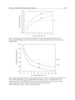
Figure 1 shows some low order Hermite-Gaussian beam modes in the rectangular
coordinate. The intensity distribution of the lowest beam mode ( 0
mn
=
= ) is Gaussian and
the Gaussian intensity profile is called either the TEM
00
mode or the fundamental mode.

2.3 Laguerre-Gaussian beam mode in cylindrical coordinate
We can also solve the differential equation (2.16) in the cylindrical coordinate with a radially
symmetric boundary condition. The solution of the wave equation in the cylindrical
coordinates has the form of a Laguerre function; thus, the solution is called the Laguerre-
Gaussian beam mode. In the cylindrical coordinates, the electric field propagating in the z-
direction is given by

(
)
(
)
(
)
(
)
()
222
2
2222
,, ,, ,, ,,
11
,, 0
Er z Er z Er z Er z
kEr z
rr
rrz
φφ φφ
φ
φ
∂∂∂∂

+
+++=
∂
∂∂∂
. (2.48)
The solution for the differential equation (2.48) has the form of Laguerre polynomials. As
such, the solution of the differential equation is given by

()
()
()
()
()
()
()
()
()
22
0
22
cos
22
,, exp
sin
n
n
mn m
m
rz rz rz
ErzE L

wz
m
wz wz
φ
φ
φ
⎛⎞⎛⎞ ⎛ ⎞
⎧⎫
⎪⎪
⎜⎟⎜⎟ ⎜ ⎟
=×××−
⎨⎬
⎜⎟⎜⎟ ⎜ ⎟
⎪⎪
⎩⎭
⎝⎠⎝⎠ ⎝ ⎠
. (2.49)
Note that some low order Laguerre polynomials are given by
(
)
0
1
l
Lx
=
,
(
)
1
1

l
Lx l x
=
+−,
(
)
(
)
(
)
(
)
2
2
122 2 2
l
Lx l l l xx=+ + −+ + ,
and
(
)
(
)
(
)
(
)
(
)
(
)

(
)
23
3
1236 232 32 6
l
Lx l l l l l x l x x=+ + + −+ + ++ − . (2.50)
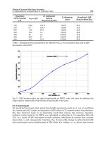
Figure 2 shows some low order Laguerre-Gaussian beam modes in the cylindrical
coordinate. Note that as for the Hermite-Gaussian beam, the lowest beam mode is Gaussian
and is also called the fundamental mode.

E
00
E
10
E
11
(sin)
E
11
(cos)
E
20
E
00
E
10
E
11
(sin)

E
11
(cos)
E
20

Fig. 2. Intensity distributions for several Laguerre-Gaussian laser beam modes.
Laser Beam Diagnostics in a Spatial Domain

215
2.4 Other beam modes
2.4.1. Flat-top beam profile and super Gaussian beam profile
In high-power laser systems, a uniform beam profile is required in order to efficiently
extract energy from an amplifier. The uniform beam profile is sometimes called a flat-top (or
top-hat) beam profile. However, the ideal flat-top beam profile is not possible because of
diffraction; in many cases, a super-Gaussian beam profile is more realistic. The definition of
the super-Gaussian beam profile is given by

22
0
exp 2
n
rw
⎡
⎤
−
⎣
⎦
. (2.51)
Here,

n is called the order of the super-Gaussian beam mode and
0
w is the Gaussian beam
radius when
n is 1. Figure 3 shows the intensity profiles for several super-Gaussian beam
profiles having different orders. As shown in the figure, the intensity profile becomes flat in
the central region as the order of the super-Gaussian beam profile increases. Note that the
flat-top beam profile is a specific case of the super-Gaussian beam profile having an order of
infinity.
0
0.2
0.4
0.6
0.8
1
1.2
Relative intensity (a.u.)
n = 1 n = 5 n = 10 n = 15 n = 20
n = 1 n = 5 n = 10
n = 15
n = 20
Position
0
0.2
0.4
0.6
0.8
1
1.2
Relative intensity (a.u.)

n = 1 n = 5 n = 10 n = 15 n = 20
n = 1 n = 5 n = 10
n = 15
n = 20
Position

Fig. 3. Intensity distributions and their line profiles for several super-Gaussian laser beam
modes having a different super-Gaussian order n.
2.4.2 Bessel-Gaussian beam profile
In this subsection, we will introduce a special laser beam mode called a Bessel beam. The
Bessel function is a solution of the wave equation (2.16) in the cylindrical coordinate. Until
1987, the existence of the Bessel laser beam was not experimentally demonstrated.
Theoretically, the Bessel laser beam has a special property that preserves its electric field
distribution over a long distance. This is why the Bessel laser beam is referred to as a
diffraction-free laser beam mode. However, in real situations, the Bessel laser beam mode
preserves its electric field distribution for a certain distance because of the infinite power
Laser Pulse Phenomena and Applications

216
problem. Now, let us derive the Bessel laser beam mode from the wave equation. The wave
equation in the cylindrical coordinate can be rewritten as

(
)
(
)
(
)
(
)

()
222
2
2222
,, ,, ,, ,,
11
,, 0
Er z Er z Er z Er z
kEr z
rr
rrz
φφ φφ
φ
φ
∂∂∂∂
+
+++=
∂
∂∂∂
. (2.48)
Then, using the separation of variables, the solution for equation (2.48) is

(
)
(
)
(
)
,, , expEr z Er i z
φ

φβ
=×−, (2.52)
and by inserting equation (2.52) into equation (2.48), equation (2.48) becomes

(
)
(
)
(
)
()
()
22
22
222
,, ,, ,,
11
,, 0
Er z Er z Er z
kErz
rr
rr
φφ φ
βφ
φ
∂∂∂
+
++−=
∂
∂∂

. (2.53)
If the electric field is radially symmetric, then the electric field
(
)
,,Er z
φ
becomes
()
,Erz
and the derivative with respect to the angular direction vanishes, i.e.,

() ()
()
()
2
2222
2
,,
,0
Erz Erz
rrkrErz
r
r
β
∂∂
+
+− =
∂
∂
. (2.54)

Note that equation (2.54) is similar to Bessel’s differential equation with an order of 0. The
Bessel’s differential equation is expressed as

() ()
()
()
2
2222
2
0
vv v
dd
Zk Zk k vZk
d
d
ρρρρρ ρ
ρ
ρ
+
+− =. (2.55)
And, the solution of equation (2.54) is given by

()
(
)
()
22
00
,expErz E J k r i z
β

β
=× − × − . (2.56)
Thus, the solution in the cylindrical coordinate for the differential equation for the electric
field is shown to be the Bessel function. Figure 4 presents the intensity distribution and
profile for the Bessel laser beam mode.
0
0.2
0.4
0.6
0.8
1
1.2
0
0.2
0.4
0.6
0.8
1
1.2
0
0.2
0.4
0.6
0.8
1
1.2

Fig. 4. Intensity distribution and its line profile for Bessel laser beam mode.
Laser Beam Diagnostics in a Spatial Domain

217
In 1987, Gori et al. introduced the Bessel-Gaussian laser beam mode to avoid the infinite
power problem. In the Bessel-Gaussian laser beam mode, the electric field is given by

()
()
()
()
2
0
000
2
0
,exp
rz
Erz E J r
wz
β
⎛⎞
⎜⎟
=× × −
⎜⎟
⎝⎠
. (2.57)
3. Intensity distribution of the focused laser beam
In the previous section, we derived the electric field distribution referred to as the laser
beam mode. In order to determine the beam quality (or propagation) factor for the laser
beam mode, we need to know the focusing property of the laser beam. The electric field
distribution of a focused laser beam can be theoretically calculated from an incident beam
profile. In this section, the calculation of the electric field distribution of a focused laser

beam is introduced. For this task, three different approaches are used: a geometrical
approach using a ray transfer matrix, a wave optics approach using diffraction theory, and a
Fourier transform approach. From the geometrical approach, the physical insight and useful
relationships for Gaussian beam parameters before and after a focusing optic can be easily
obtained. However, if the incident beam profile is not Gaussian and has a wavefront
aberration, it becomes more difficult to use the geometrical approach to explain the focusing
property of the laser beam. In this case, the wave optics approach using diffraction theory
gives more accurate calculation results. The wave optics approach offers analytic solutions
for a Gaussian and uniform laser beams. However, the wave optics approach does not
provide an analytical solution for an arbitrary incident laser beam mode. In this case, the
Fourier transform approach becomes very useful. By using the Fourier transform method,
the electric field distribution of the focused laser beam can be easily obtained and, together
with the focus shift method, the electric field distribution near the focal plane can be quickly
obtained. In particular, the Fourier transform approach is more useful for a laser beam
having a wavefront aberration.
3.1 Geometrical approach
Propagation of the electric field can be described by the ray transfer matrix of an optical
element. The ray transfer matrix determines the deviation angle at a location of the optical
element; this matrix is also called the ABCD matrix and is expressed by

AB
CD
⎡
⎤
⎢
⎥
⎣
⎦
. (3.1)
Let us now consider the case in which a Gaussian laser beam passes through an optical

element having ABCD elements. The Gaussian beam mode [
(
)
1111
,,Exyz ] before the optical
element is again

()
()
()
22
11
1111 1
1
,, exp
2
xy
Exyz Az ik
qz
⎡
⎤
+
=×−
⎢
⎥
⎢
⎥
⎣
⎦
and

() ()
()
2
11
11
11
i
qz Rz
wz
λ
π
=− . (3.2)
Then, when the Gaussian laser beam passes through the optical element, the electric field
right after the optical element is determined by
Laser Pulse Phenomena and Applications

218

()()
()
()
()
()
222
221 1 1 1 2 12 1
1
22
112121
1
,exp exp 2

2
exp 2
2
ik
Exz Az x i Ax Dx xx dx
qz B
ik i
Az Ax i Dx i xx dx
qz B B B
π
λ
πππ
λλλ
⎡⎤
⎡⎤
−−+−
⎢⎥
⎢⎥
⎣⎦
⎢⎥
⎣⎦
⎡⎤
⎛⎞
⎢⎥
=−+−+
⎜⎟
⎜⎟
⎢⎥
⎝⎠
⎣⎦

∫
∫
∼
. (3.3)

Here, only the electric field in the x-direction is considered, though the electric field in the y-
direction can be calculated in the same manner. After some calculation, the electric field
after the optical element is given by

()
2
22 2
1
1
1
exp
2
2
ik
Ex x D
ik i
BBqA
A
qB
π
π
λ
⎡⎤
⎛⎞
=−+

⎢⎥
⎜⎟
⎜⎟
+
⎢⎥
⎝⎠
⎣⎦
+
. (3.4)
The following definite integral formula (3.5) is used to derive equation (3.4).

()
2
2
exp 2 exp
b
ax bx dx
aa
π
∞
−∞
⎛⎞
−− =
⎜⎟
⎜⎟
⎝⎠
∫
. (3.5)
Because the determinant of the matrix is 1 (i.e., 1
AD BC

−
= ), the electric field distribution
after the optical element can be rewritten as follows:

()
2
1
22 2
1
1
exp
2
2
qC D
ik
Ex x
ik i
qA B
A
qB
π
π
λ
⎡
⎤
⎛⎞
+
=−
⎢
⎥

⎜⎟
⎜⎟
+
⎢
⎥
⎝⎠
⎣
⎦
+
. (3.6)
By defining
2
1
q
as
1
1
q
CD
q
AB
+
+
, the resultant electric field distribution again has the same
expression as the incident electric field except for the laser beam parameter
2
q
, such that

()

2
22 2
2
exp
2
ik
Ex x
q
⎡⎤
−
⎢⎥
⎣⎦
∼ . (3.7)

Again, let us assume the Gaussian laser beam is focused by a focusing optic having a focal
length of
f
. Then, we need to determine the electric field distribution at the focal plane of
the focusing optic; the ray transfer matrix for a focusing optic and a free distance is given by

1100
01 1 1 1 1
AB
ff
CD f f
⎡
⎤⎡ ⎤⎡ ⎤⎡ ⎤
==
⎢
⎥⎢ ⎥⎢ ⎥⎢ ⎥

−−
⎣
⎦⎣ ⎦⎣ ⎦⎣ ⎦
. (3.8)
If the incident Gaussian laser beam is an ideal plane wave (i.e.
(
)
1
Rz
=
∞ ),
(
)
1
q
z is simply
defined as
(
)
2
11
wz
i
π
λ
. Then,
2
1
q
can be quickly calculated as

Laser Beam Diagnostics in a Spatial Domain

219
For a Gaussian laser beam
1
w
1100
01 1 1 1 1
f
f
ff
⎡
⎤⎡ ⎤ ⎡ ⎤
=
⎢
⎥⎢ ⎥ ⎢ ⎥
−−
⎣
⎦⎣ ⎦ ⎣ ⎦
ABCD matrix
2
1
f
w
w
λ
π
=
Focal length = f
Distance = f

For a Gaussian laser beam
1
w
1100
01 1 1 1 1
f
f
ff
⎡
⎤⎡ ⎤ ⎡ ⎤
=
⎢
⎥⎢ ⎥ ⎢ ⎥
−−
⎣
⎦⎣ ⎦ ⎣ ⎦
ABCD matrix
2
1
f
w
w
λ
π
=
Focal length = f
Distance = f

Fig. 5. Focusing Gaussian laser beam mode having a focusing optic with a focal length of
f

.
2
1
22
22
2
11 11w
ii
q
R
f
wf
λπ
λ
π
=
−=− +. (3.9)
Thus, the intensity profile of a focused Gaussian beam is again Gaussian with a new
Gaussian width
2
w , which is given by

1
2
2
1
R
f
w
f

w
w
z
λ
π
==
, (3.10)
where
R
z is defined as
1
2
2
1
R
f
w
f
w
w
z
λ
π
== and called the Rayleigh range, at which point the
area of the laser beam increases by a factor of 2. The electric field distribution near the focal
plane can be calculated by replacing the focal length
f
with the distance d in equation
(3.8). However, even if an arbitrary optical element having an arbitrary wavefront
aberration can be represented by a ray transfer matrix, the general description of the electric

field distribution for an arbitrary electric field cannot be simply expressed by the
geometrical approach.
3.2 Wave optics approach using diffraction theory
Now, in this section, we will directly calculate the electric field distribution based on the
diffraction integral. Again, consider that an electric field converges from a focusing optic
having a focal length of
f
to the axial focal point. Then, the electric field distribution at a
point (
2
x ,
2
y ) in the focal plane is given by

() ()
22 111 11
,,
ikf
iks
ie e
E x y E x y dx dy
fs
λ
−
=−
∫
. (3.11)
Laser Pulse Phenomena and Applications

220

111
,Exy
⎛⎞
⎜⎟
⎝⎠
1
y
1
x
2
y
2
x
Focusing optic
Focal plane
f
s
22
,Ex y
⎛⎞
⎜⎟
⎝⎠
z
q

R

111
,Exy
⎛⎞

⎜⎟
⎝⎠
1
y
1
x
2
y
2
x
Focusing optic
Focal plane
f
s
22
,Ex y
⎛⎞
⎜⎟
⎝⎠
z
q

R


Fig. 6. Diffraction of electric field at a focusing optic having a focal length
f
.
To evaluate equation (3.11), let us assume that the focusing optic is circular and that the
radius of the focusing optic is a . Then, it is convenient to express (

1
x ,
1
y ,
1
z ) and
(
2
x ,
2
y ,
2
z ) in the cylindrical coordinate as follows:

1
sinxa
ρ
θ
=
,
1
cosya
ρ
θ
=
, and
2
sinxr
ϕ
=

,
2
cosyr
ϕ
=
(3.12)
where
ρ
extends from zero to 1. In this expression, from Fig. 6, the difference sf− and the
small area of
11
dx dy can be, via an approximation, expressed as
s
fq
R
−
=− ⋅


and
2
11
dx d
yf
d
=
Ω (3.13)
where d
Ω is the infinitesimal solid angle. Then, using the approximation sf
≈

, the electric
field distribution at a point (
2
x ,
2
y
) becomes

() ()
22 111
,,
kq R
i
Ex y E x y e d
λ
−⋅
=
−Ω
∫


. (3.14)
Equation (3.14) is known as the Debye integral and expresses the electric field as a
superposition of plane wave components having different directions of propagation, known
as angular spectrums. The phase component in the integral is

12 12 12
xx
yy
zz

qR
f
++
⋅=


, (3.15)
and the axial position
1
z of element
11
dx dy from the origin of (
2
x ,
2
y
,
2
z ) is

22 44
222
1
24
13
1
28
aa
zfa f
ff

ρρ
ρ
⎡
⎤
=− − =− − + −
⎢
⎥
⎢
⎥
⎣
⎦

. (3.16)
Laser Beam Diagnostics in a Spatial Domain

221
By inserting equation (3.16) into equation (3.15) and using
f
a , we obtain the following
expression for the phase component in the Debye integral:

(
)
22
12 12 12
2
cos
221
1
2

ar
xx yy zz
a
kq R k z
ff
f
ρθϕ
π
πρ
λλ
⎡
⎤
−
++
⋅= = − −
⎢
⎥
⎢
⎥
⎣
⎦


. (3.17)
Then, by introducing dimensionless variables u and v in the focal plane, defined as

2
2 a
uz
f

π
λ
⎛⎞
=
⎜⎟
⎜⎟
⎝⎠
and
2 a
vr
f
π
λ
⎛⎞
=
⎜⎟
⎜⎟
⎝⎠
, (3.18)
the phase component in the Debye integral is

()
2
2
1
cos
2
f
k
q

Rv u u
a
ρ
θϕ ρ
⎛⎞
⋅= − − +
⎜⎟
⎝⎠


. (3.19)
Thus, equation (3.14), which expresses the electric field distribution in the focal plane, becomes

() () ( )
2
2
12
2
2
00
1
,exp ,expcos
2
f
ia
Euv i u E iv u d d
a
f
π
ρ

θρθϕρρρθ
λ
⎡⎤
⎧⎫
⎛⎞
⎡⎤
⎢⎥
=− − − +
⎨⎬
⎜⎟
⎢⎥
⎢⎥
⎣⎦
⎝⎠
⎩⎭
⎣⎦
∫∫
.(3.20)
And, if the incoming electric field is radially symmetric, equation (3.20) can be simply
expressed as

() () ( )
2
2
1
2
0
2
0
21

,exp exp
2
f
ia
Euv i u E J v i u d
a
f
π
ρ
ρρρρ
λ
⎡⎤
⎛⎞
⎡⎤
⎢⎥
=− −
⎜⎟
⎢⎥
⎢⎥
⎣⎦
⎝⎠
⎣⎦
∫
, (3.21)
using the definition of Bessel function.

() ()
2
0
0

1
exp cos
2
Jx ix d
π
θ
θ
π
=
∫
. (3.22)
If we consider the uniform intensity profile, then the incoming electric field is constant with
respect to the position (i.e.
(
)
,EC
ρθ
=
). In this case, the electric field distribution in the
focal plane has the form

() ()
2
2
1
2
0
2
0
21

,exp exp
2
f
aC
Euv i i u J v iu d
a
f
π
ρ
ρρρ
λ
⎡⎤
⎛⎞
⎛⎞
⎢⎥
=− −
⎜⎟
⎜⎟
⎢⎥
⎝⎠
⎝⎠
⎣⎦
∫
. (3.23)
To calculate equation (3.35) further, we separate the integral into the real and imaginary
parts.
() () ()
2
2
11

22
00
2
00
211
,exp cos sin
22
f
aC
Euv i i u J v u d i J v u d
a
f
π
ρ
ρρρ ρ ρρρ
λ
⎡⎤
⎡
⎤
⎛⎞
⎛⎞ ⎛⎞
⎢⎥
=− −
⎢
⎥
⎜⎟
⎜⎟ ⎜⎟
⎢⎥
⎝⎠ ⎝⎠
⎝⎠

⎣
⎦
⎣⎦
∫∫
. (3.24)
Laser Pulse Phenomena and Applications

222
There are two different cases in evaluating the integrals in equation (3.24). In the first case,
when
/1uv< (i.e. inside the geometrical shadow), we use the relation for the Bessel
function to obtain
() ()
11
22
01
00
12 1
2cos cos
22
d
Jv ud Jv ud
vd
ρ
ρρρ ρ ρ ρρρ
ρ
⎛⎞ ⎛⎞
⎡⎤
=
⎜⎟ ⎜⎟

⎣⎦
⎝⎠ ⎝⎠
∫∫


() ()
()
() ()
()
() ()
()
()
()
()
1
22
11
0
324
13 24
12
21 1
cos sin
22
cos 2 sin 2
22
cos 2 sin 2
,,
22
Jv u u Jv u d

v
uu
uu u u
Jv Jv Jv Jv
uv v uv v
uu
Uuv Uuv
uu
ρρ ρρρ
⎡⎤
⎛⎞ ⎛ ⎞
=+
⎢⎥
⎜⎟ ⎜ ⎟
⎝⎠ ⎝ ⎠
⎣⎦
⎡
⎤⎡ ⎤
⎛⎞ ⎛⎞ ⎛⎞ ⎛⎞
⎢
⎥⎢ ⎥
=−++ −+
⎜⎟ ⎜⎟ ⎜⎟ ⎜⎟
⎢
⎥⎢ ⎥
⎝⎠ ⎝⎠ ⎝⎠ ⎝⎠
⎣
⎦⎣ ⎦
=+
∫


. (3.25)
where the following definition of the Lommel function
(
)
,
n
Uuv and the relation for the
Bessel function are used to obtain equation (3.25):

() () ()
2
2
0
,1
ns
s
nns
s
u
Uuv J v
v
+
∞
+
=
⎛⎞
=−
⎜⎟
⎝⎠

∑
, (3.26)
and
() ()
11
1
nn
nn
d
xJ x xJx
dx
++
+
⎡⎤
=
⎣⎦
. (3.27)
In a similar way, we obtain the expression for the imaginary part:

()
(
)
()
(
)
()
1
2
012
0

sin 2 cos 2
1
2sin , ,
22 2
uu
Jv u d Uuv Uuv
uu
ρρρρ
⎛⎞
=−
⎜⎟
⎝⎠
∫
. (3.28)
In the second case, when
/1uv> (i.e. outside the geometrical shadow), we evaluate
equation (3.24) by integrating by parts with respect to the trigonometric function in order to
finally obtain the expressions for the real and imaginary parts as follows:

()
(
)
()
()
()
()
2
1
2
001

0
sin 2
sin 2 cos 2
1
2cos , ,
2222
vu
uu
Jv u d Vuv Vuv
uu u
ρρρρ
⎛⎞
=+ −
⎜⎟
⎝⎠
∫
, (3.29)
and
()
(
)
()
()
()
()
2
1
2
001
0

cos 2
cos 2 sin 2
1
2sin , ,
2222
vu
uu
Jv u d Vuv Vuv
uu u
ρρρρ
⎛⎞
=− −
⎜⎟
⎝⎠
∫
. (3.30)
The other definition of the Lommel function,
(
)
,
n
Vuv, is then used for obtaining equations
(3.29) and (3.30).

() () ()
2
2
0
,1
ns

s
nns
s
v
Vuv J v
u
+
∞
+
=
⎛⎞
=−
⎜⎟
⎝⎠
∑
. (3.31)
Laser Beam Diagnostics in a Spatial Domain

223

2
2 a
uz
f
π
λ
⎛⎞
⎜⎟
⎜⎟
⎝⎠

=
2 a
vr
f
π
λ
⎛⎞
⎜⎟
⎜⎟
⎝⎠
=
2
2 a
uz
f
π
λ
⎛⎞
⎜⎟
⎜⎟
⎝⎠
=
2 a
vr
f
π
λ
⎛⎞
⎜⎟
⎜⎟

⎝⎠
=

Fig. 7. Intensity distribution near the focal plane calculated using the diffraction integral
approach when a flat-top beam profile is focused.
Now, let us calculate the electric field distribution in the focal plane from equations (3.21),
(3.25), (3.28), (3.29), and (3.30). First, in the region
/1uv
<
, we use equations (3.21), (3.25),
and (3.28) to calculate the intensity distribution.

()
() ()
22
12
0
2
,,
,4
Uuv Uuv
Iuv I
u
⎡
⎤
+
=
⎢
⎥
⎢

⎥
⎣
⎦
. (3.32)
Figure 7 shows the intensity distribution near the focal plane calculated using equation
(3.32) when a flap-top laser beam is focused. In the special case of a focal plane ( 0u
= ), the
intensity distribution is

()
(
)
2
1
0
2
0, 4
Jv
Iv I
v
= . (3.33)
Thus, as shown in equation (3.33), the Airy function is obtained when we focus a uniform
electric field. If the incoming laser beam has a Gaussian beam profile, then the electric field
distribution in equation (3.21) has the form

()
22
1
2
0

exp
a
EC
w
ρ
ρ
⎡
⎤
=× −
⎢
⎥
⎢
⎥
⎣
⎦
. (3.34)
In equation (3.34), we only consider the case of a plane wave (i.e.
R
=
∞ ). By inserting
equation (3.34) into equation (3.21), equation (3.21) becomes

() ()
()
2
222
1
2
0
22

0
0
2
1
2
0
2
0
0
21
,expexp exp
2
exp
2
f
iaC a
Euv i u J v i u d
a
fw
au
Jv i d
w
πρ
ρ
ρρρ
λ
ρρρρ
⎡⎤
⎡⎤
⎛⎞

⎡⎤
⎢⎥
=− − −
⎢⎥
⎜⎟
⎢⎥
⎢⎥
⎣⎦
⎝⎠
⎢⎥
⎣⎦
⎣⎦
⎡⎤
⎛⎞
≈−+
⎢⎥
⎜⎟
⎜⎟
⎢⎥
⎝⎠
⎣⎦
∫
∫
. (3.35)
Laser Pulse Phenomena and Applications

224
Again, in the special case of a focal plane ( 0u
=
), the electric field distribution in the focal

plane is

() ()
22
1
0
2
0
0
0, exp
a
Ev Jv d
w
ρ
ρ
ρρ
⎛⎞
≈−
⎜⎟
⎜⎟
⎝⎠
∫
. (3.36)
To integrate equation (3.36), we use the following definite integral formula:

()
()()
22
2
0

1
exp exp
242
mm m
x I x J x xdx J
β
γβγ
αβγ
α
αα
∞
⎛⎞
−
⎛⎞
−=
⎜⎟
⎜⎟
⎜⎟
⎝⎠
⎝⎠
∫
. (3.37)
The small beam size approximation (
0
aw ) is used to apply the definite integral formula.
Then, the final expression for the incoming Gaussian beam is

() ()
2222
22 2

1
000
0
22222
0
01
0, exp exp exp
242
wwvw
ar
Ev Jv d
waaaw
ρ
ρρρ
⎛⎞ ⎛⎞
⎛⎞
≈ − =−=−
⎜⎟ ⎜⎟
⎜⎟
⎜⎟
⎜⎟ ⎜⎟
⎝⎠
⎝⎠ ⎝⎠
∫
. (3.38)
From equation (3.38), the new Gaussian beam size for the focused electric field is obtained as

1
0
f

w
w
λ
π
= . (3.39)
Obviously, the new Gaussian beam size for the focused electric field calculated from the
Debye integral is exactly the same as that calculated from the geometrical approach. Unlike
the above special cases (uniform and Gaussian field profiles), an analytical solution for the

Geometric optics approach
Focusing
Optic
Geometric
shadow
Focal plane
x
z
Gaussian Flat-top
Wave optics approach
Gaussian
Flat-top
Geometric
shadow
x
z
x
z
Rayleigh range
(Depth of focus)
Geometric optics approach

Focusing
Optic
Geometric
shadow
Focal plane
x
z
Gaussian Flat-top
Geometric optics approach
Focusing
Optic
Geometric
shadow
Focal plane
x
z
Gaussian Flat-top
Focusing
Optic
Geometric
shadow
Focal plane
x
z
Gaussian Flat-top
Wave optics approach
Gaussian
Flat-top
Geometric
shadow

x
z
x
z
Rayleigh range
(Depth of focus)
Wave optics approach
Gaussian
Flat-top
Geometric
shadow
x
z
x
z
Rayleigh range
(Depth of focus)
Gaussian
Flat-top
Geometric
shadow
x
z
x
z
Rayleigh range
(Depth of focus)

Fig. 8. Focusing laser beam: geometrical optics and wave optics approaches.
Laser Beam Diagnostics in a Spatial Domain

225
focused electric field does not exist for an electric field having an arbitrary magnitude and
wavefront. Thus, in case of an arbitrary electric field, it is convenient to use the Fourier
transform approach to calculate the focused electric or intensity distribution in and near the
focal plane.
3.3 Fourier transform approach
If we assume that a laser beam is focused with an ideal focusing optic having a focal length
f
, then the electric field distribution at the focal plane can be expressed by

() () () ()
2 22 111 11 12 12 11
,,exp,exp
k
Ex
y
Ex
y
ikW x
y
ixx
yy
dx d
y
f
∞
−∞
⎡⎤
⎡⎤

+
⎢⎥
⎣⎦
⎣⎦
∫
∼ . (3.40)
This integral form represents the Fourier transform of the incident electric field having an
arbitrary wavefront aberration
(
)
11
,Wx y . Now, let us quickly review the derivation of
equation (3.40). Consider that a monochromatic electric field
(
)
111
,Exy converges by a
focusing optic having a focal length
f to the axial focal point. Again, the electric field
distribution at a point (
2
x ,
2
y
) in the focal plane is given by

() ()
22 111 11
,,
ikf

iks
ie e
E x y E x y dx dy
fs
λ
−
=−
∫
(3.11)
where
1
x and
1
y are the coordinates in the aperture plane, and s is the distance from a
certain point in the focusing optic to the point (
2
x ,
2
y
). Then, if we express s in the (x, y)
coordinate, s is

()
()
22
2
2
2
12
12

12 12 2 2
22
22
12
12
2
22
1
11
1
22
yy
xx
sxx yy zz
zz
yy
xx
z
zz
⎛⎞⎛⎞
−
−
=−+−+=+ +
⎜⎟⎜⎟
⎜⎟⎜⎟
⎝⎠⎝⎠
⎡⎤
⎛⎞⎛⎞
−
−

⎢⎥
≈+ +
⎜⎟⎜⎟
⎜⎟⎜⎟
⎢⎥
⎝⎠⎝⎠
⎣⎦
. (3.41)
Because the phase of the electric field varies more quickly than the magnitude, we can
approximate
s such that
2
sz f
≈
≈
in the expression related to the magnitude. Thus,
equation (3.11) becomes
()
()
()
()
()
22 22
22 2 2 111 1 1 12 12 11
2
, exp , exp exp
22
ikf
ie ik ik k
E x y x y E x y x y x x y y dx dy

fff
f
λ
−
⎡⎤ ⎡⎤⎡ ⎤
=− + + − +
⎢⎥ ⎢⎥⎢ ⎥
⎣⎦ ⎣⎦⎣ ⎦
∫
. (3.42)
We then derive the expression for electric field distribution in a focal plane when the electric
field is focused with a focusing optic having a focal length
f
. In equation (3.42), one
important consideration is the phase delay due to the focusing optic; the phase function
including phase delay should be considered in the electric field
(
)
111
,Exy
. For this task, we
first have to obtain the expression for the phase delay. If we consider a lens having the
thickness shown in Fig. 9, then the phase delay after the lens is