báo cáo hóa học: " Synchronization of nonidentical chaotic neural networks with leakage delay and mixed timevarying delays" pptx
Bạn đang xem bản rút gọn của tài liệu. Xem và tải ngay bản đầy đủ của tài liệu tại đây (815.92 KB, 17 trang )
RESEARC H Open Access
Synchronization of nonidentical chaotic neural
networks with leakage delay and mixed time-
varying delays
Qiankun Song
1
and Jinde Cao
2*
* Correspondence:
cn
2
Department of Mathematics,
Southeast University, Nanjing
210096, China
Full list of author information is
available at the end of the article
Abstract
In this paper, an integral sliding mode control approach is presented to investigate
synchronization of nonidentical chaotic neural networks with discrete and distributed
time-varying delays as well as leakage delay. By considering a proper sliding surface
and constructing Lyapunov-Krasovskii functional, as well as employing a combination
of the free-weighting matrix method, Newton-Leibniz formulation and inequality
technique, a sliding mode controller is designed to achieve the asymptotical
synchronization of the addressed nonidentical neural networks. Moreover, a sliding
mode control law is also synthesized to guarantee the reachability of the specified
sliding sur face. The provided conditions are expressed in terms of linear matrix
inequalities, and are dependent on the discrete and distributed time delays as well
as leakage delay. A simulation example is given to verify the theoretical results.
Keywords: Synchronization, Chaotic neural network, Leakage delay, Discrete time-
varying delays, Distributed time-varying delays 05.45.Xt 05.45.Gg
Introduction
In the past few years, neural networks have attracted much attention due to the bac k-
ground of a wide range applications such as associative memory, pattern recognition,
image processing and model identification [1]. In such applications, the qualitative ana-
lysis of the dynamical behaviors is a necessary step for the practical design of neural
networks [2].
In hardware implementation, time delays occur due to finite switching speed of the
amplifiers and communication time. The existence of time delay may lead to some
complex dynamic behaviors such as oscillation, divergence, chao s, instability, or other
poor performance of the neural networks [3]. Therefore, the study of dynamical beha-
viors with consideration of time delays becomes extremely important to m anufacture
high-quality neural networks [4]. Many results on dynamical behaviors have been
reported for delayed neural networks, for example, see [1-10] and references therein.
On the other hand, it was found that some delayed neural networks can exhibit
chaotic behavior [11-13]. These kinds of chaotic neural networks have been utilized to
solve optimization problems [14]. Since the drive-response concept for considering
synchronization of coupled chaotic systems was proposed in 1990 [15], the synchroni-
zation of chaotic systems has attracted considerable attention due to its benefits of
Song and Cao Advances in Difference Equations 2011, 2011:16
/>© 2011 Song and Cao; licensee Spr inger. This is an Open Access article dis trib uted under the terms of the Creative Commons
Attribution License ( nses/by/2.0), which permits unrestricted use, distr ibution, and reproduction in
any medium, provided the original work is properly cited.
having chaos synchronization in some engineering applications such as secure commu-
nication, chemical reactions, information processing and harmonic oscillation genera-
tion [16]. Therefore, some chaotic neural networks with delays could be treated as
models when we study the synchronization.
Recently, some works dealing w ith synchronization phenomena in de layed neural
networks have also appeared, for example, see [17-29] and references therein. In
[17-20], the coupled connected neural networks with delays were c onsidered, several
sufficient conditions for synchronization of such neural networks were obtained by
Lyapunov stability theory and the li near matrix inequality (LMI) technique. In [21-29],
the authors investigated the synchronization problem of some chaotic neural networks
with delays. Using the drive-response concept, the control laws were derived to achieve
the synchronization of two identical chaotic neural networks.
It is worth pointing out that, the reported works in [17-29] focused on synchronizing
of two identical chao tic neural networks with different initial conditi ons. In practice,
the chaotic systems are inevitably subject to some environmental changes, which may
render their parameters to be variant. Furthermore, from the point of view of engineer-
ing, it is very difficult to keep the two chaotic systems to be identical all the time.
Therefore, it is important to study the synchronization problem of nonidentical chaotic
neural networks. Obviously, when the considered drive a nd response neural networks
are distinct and with time delay, it becomes more complex and challenging. On the
study for synchronization problem of two nonidentical chaotic systems, one usually
adopts adaptive control approach to establish synchronization conditions, for example,
see [30-32], and refere nces therein. Recently, the integral sliding mode control
approach is also employed to investigate synchronization of nonidentical chaotic
delayed neura l networks [33-38]. In [33], an integral sliding mode control appr oach is
proposed to address synchronization for two nonidentical chaotic neural networks with
constant delay. Based on the drive-response concept and Lyapunov stability t heory,
both delay-independent and delay-dependent conditions in LMIs are derived under
which the resulting error system is globally asymptotically stable in the specified
switc hing surface, and a sliding mode controller is synthesized to guarantee the reach-
ability of the specified sliding surface. In [34], the authors investigated synchronization
for two chaotic neural networks with discrete and distributed constant delays. By using
Lyapunov functional method and LMI technique, a delay-dependent condition was
obtained to ensure that the drive system synchronizes with the identical response sys-
tem. When the parameters and activation functions of two chaotic neural networks
mismatched, the synchronization criterion is also derived by sliding mode control
approach. In [35], the projective synchronization for two nonidentical chaotic neural
networks with constant delay was investigated, a delay-dependent sufficient condition
was derived by sliding mode control approach, LMI technique and Lyapunov stability
theory. However, to the best of the authors’ knowledge, there are no results on the
problem of synchronization for chaotic neural networks with leakag e delay. As pointed
out in [39], neural networks with leakage delay is a class of important neural networks;
time delay in the leakage term also has great impact on the dynamics of neural net-
works because time delay in the stabilizing negative feedback term has a tendency to
destabilize a system [39-43]. Therefore, it is necessary to further investigate the syn-
chronization problem for two chaotic neural networks with leakage delay.
Song and Cao Advances in Difference Equations 2011, 2011:16
/>Page 2 of 17
Motivated by the above discussions, the objective of this paper is to present a sys-
tematic design procedure for synchronization of two nonidentical chaotic neural net-
works with discrete and distributed time-varying delays as well as leakage delay. By
constructing a proper sliding surface and Lyapunov-Krasovskii functional, and employ-
ing a combination of the free-weighting matrix method, Newton-Leibniz formulation
and inequality technique, a sliding mode controller is designed to achieve the asympto-
tical synchroni zation of the addressed nonidentical neural networks. Moreo ver, a sli d-
ing mode control law is a lso synthesized to guarantee the reachability of the specified
sliding surface. The provided conditions are expressed in terms of LMI, and are depen-
dent on the discrete and distributed time delays as well as leakage delay. Differing from
the results in [33-35], the main contributions of this study are to investi gate the effect
of the leakage delay on the synchronization of two nonidentical chaotic neural net-
works with discrete and distributed time-varying delays as well as leakage delay and to
propose an integral sliding mode control approach to solving it.
Problem formulation and preliminaries
In this paper, we consider the following neural network model
˙
y(t )=− D
1
y(t − δ)+A
1
f (y(t)) + B
1
f (y(t − τ(t ))
)
+ C
1
t
t−σ
(
t
)
f (y(s))ds + I
1
(t ), t ≥ 0,
(1)
where y(t)=(y
1
(t), y
2
(t), , y
n
(t))
T
Î R
n
is the state vector of the network at time t, n
corresponds to the number of neurons; D
1
Î R
n × n
is a positive diagonal matrix, A
1
,
B
1
, C
1
Î R
n × n
are, respectively, the connection weight matrix, the discretely delayed
connection weight matrix and distributively delayed connection weight matrix; f(y(t)) =
(f
1
(y
1
(t)), f
2
(y
2
(t)), , f
n
(y
n
(t)))
T
Î R
n
denotes the neuron activation at time t; I
1
(t) Î R
n
is an external input vector; δ ≥ 0, τ(t) ≥ 0ands(t) ≥ 0 denote the leakage delay, the
discrete time-varying delay and the distributed time-varying dela y, respectively, and
sati sfy 0 ≤ τ(t) ≤ τ,0≤ s(t) ≤ s,whereδ, τ and s are constants. It is assumed that the
measured output of system (1) is dependent on the state and the delayed states with
the following form:
w
(
t
)
= K
1
y
(
t
)
+ K
2
y
(
t − δ
)
+ K
3
y
(
t − τ
(
t
))
+ K
4
y
(
t − σ
(
t
)),
(2)
where w(t) Î R
m
, K
i
Î R
m × n
(i = 1, 2, 3, 4) are known constant matrices.
The initial condition associated with model (1) is given by
y
(
s
)
= φ
(
s
)
, s ∈ [−ρ,0]
,
where j(s) is bounded and continuously differential on [-r, 0], r = max {δ, τ, s}.
We consider the system (1) as the drive system. The response system is as follows:
˙
z
(t )=− D
2
z(t − δ)+A
2
g(z(t)) + B
2
g(z(t − τ(t))
)
+ C
2
t
t−σ
(
t
)
g(z(s))ds + I
2
(t )+u(t), t ≥ 0,
(3)
with initial condition z(s)=(s), s Î [-r, 0], where (s) is bounded and continuously
differential on [-r,0],u(t) is the appropriate control input that will be designed in
order to obtain a certain control objective.
Song and Cao Advances in Difference Equations 2011, 2011:16
/>Page 3 of 17
Let x(t)=y(t)-z(t) be the error state, then the error system can be obtained from
(1) and (3) as follows:
˙
x(t )=− D
1
x(t − δ)+A
1
h(x(t)) + B
1
h(x(t − τ (t))) + C
1
t
t−σ (t)
h(x(s))d
s
+(D
2
− D
1
)z(t − δ) − A
2
g(z(t)) − B
2
g(z(t − τ(t)))
− C
2
t
t−σ (t)
g(z(s))ds + A
1
f (z(t)) + B
1
f (z(t − τ (t)))
+ C
1
t
t−σ
(
t
)
f (z(s))ds − u(t)+I
1
(t ) − I
2
(t ),
(4)
where h(x(t)) = f(y(t)-f(z(t)), and x(s)=j(s)-(s), s Î [-r, 0].
Definition 1 Thedrivesystem(1)andtheresponsesystem(3)issaidtobeglobally
asymptotically synchronized, if system (4) is globally asymptotically stable.
The aim of the paper is to design a controller u(t) to let the response system (3) syn-
chronize with the drive system (1).
Since dynamic behavior of error system (4) relies on both error state x(t) and chaotic
state z(t) of response system (3), complete synchronization between two nonidentical
chaotic neural networks ( 1) and (3) cannot b e achieved only by utilizing output feed-
back control. To overcome the difficulty, an integral sliding mode c ontrol approach
will be proposed to investigate the synchronization problem of two nonidentical chao-
tic neural networks (1) and (3). In other words, an integral slid ing mode controller is
designed such that the sliding motion is globally asymptotically stable, and the state
trajectory of the error system (4) is globally driven onto the specified sliding surface
and maintained there for all subsequent time.
To utilize the information of the measured output w(t), a suitable sliding surface is
constructed as
S(t )=x(t)+
t
0
D
1
x(ξ − δ) − A
1
h(x(ξ)) − B
1
h(x(ξ − τ (ξ)))
− C
1
ξ
ξ−σ (ξ )
h(x(s))ds + K
w(ξ) − K
1
z(ξ) − K
2
z(ξ − δ
)
− K
3
z(ξ − τ (ξ)) − K
4
z(ξ − σ (ξ ))
dξ,
(5)
where K Î R
n × m
is a gain matrix to be determined.
It follows from (2), (4) and (5) that
S(t )=x(0) +
t
0
(D
2
− D
1
)z(ξ − δ) − A
2
g(z(ξ )) − B
2
g(z(ξ − τ(ξ))
)
− C
2
ξ
ξ−σ (ξ )
g(z(s))ds + A
1
f (z(ξ)) + B
1
f (z(ξ − τ (ξ)))
+ C
1
ξ
ξ−σ (ξ )
f (z(s))ds − u(ξ)+I
1
(ξ) − I
2
(ξ)+KK
1
x(ξ)
+ KK
2
x(ξ − δ)+KK
3
x(ξ − τ(ξ )) + KK
4
x(ξ − σ(ξ ))
dξ.
(6)
According to the sliding mode control theory [44], it is true that S(t)=0and
˙
S
(
t
)
=
0
as the state trajectories of the error system (4) enter into the sliding mode. It
Song and Cao Advances in Difference Equations 2011, 2011:16
/>Page 4 of 17
thus follows from (6) and
˙
S
(
t
)
=
0
that an equivalent control law can be designed as
u
(t )=(D
2
− D
1
)z(t − δ) − A
2
g(z(t)) − B
2
g(z(t − τ(t)))
− C
2
t
t−σ (t)
g(z(s))ds + A
1
f (z(t)) + B
1
f (z(t − τ (t)))
+ C
1
t
t−σ (t)
f (z(s))ds + I
1
(t ) − I
2
(t )
+ KK
1
x
(
t
)
+ KK
2
x
(
t − δ
)
+ KK
3
x
(
t − τ
(
t
))
+ KK
4
x
(
t − σ
(
t
)).
(7)
Substituting (7) into (4), the sliding mode dynamics can be obtained and described
by
˙
x(t )=− KK
1
x(t ) − (D
1
+ KK
2
)x(t − δ) − KK
3
x(t − τ (t)) − KK
4
x(t − σ (t)
)
+ A
1
h(x(t)) + B
1
h(x(t − τ (t))) + C
1
t
t−σ
(
t
)
h(x(s))ds.
(8)
Throughout this paper, we make the following assumption:
(H). For any j Î {1, 2, , n}, there exist constants
F
−
j
,
F
+
j
,
G
−
j
and
G
+
j
such that
F
−
j
≤
f
j
(α
1
) − f
j
(α
2
)
α
1
− α
2
≤ F
+
j
, G
−
j
≤
g
j
(α
1
) − g
j
(α
2
)
α
1
− α
2
≤ G
+
j
for all a
1
≠ a
2
.
To prove our result, the following lemma that can be found in [41] is necessary.
Lemma 1 For any constant matrix W Î R
m × m
, W >0,scalar 0 <h(t) <h,vector
function ω : [0, h] ® R
m
such that the integrations concerned are well defined, then
h(t)
0
ω(s )ds
T
W
h(t)
0
ω(s )ds
≤ h( t)
h(t)
0
ω
T
(s)Wω(s)ds
.
Main results
For presentation convenience, in the following, we denote
F
1
= diag(F
−
1
, F
−
2
, , F
−
n
), F
2
= diag(F
+
1
, F
+
2
, , F
+
n
)
,
F
3
= diag(F
−
1
F
+
1
, F
−
2
F
+
2
, , F
−
n
F
+
n
),
F
4
= diag(
F
−
1
+ F
+
1
2
,
F
−
2
+ F
+
2
2
, ,
F
−
n
+ F
+
n
2
).
Theorem 1 Assume that the condition (H) holds and the measured output of drive
neural network (1) is condition (2). If there exist five symmetric positive definite
matrices P
i
(i =1,2,3,4,5), four positive diagonal matr ices R
i
(i =1,2,3,4), and ten
matrices M, N, L, Y, X
ij
(i, j =1,2,3,i ≤ j) such that the following two LMIs hold:
X =
⎡
⎣
X
11
X
12
X
13
X
T
12
X
22
X
23
X
T
13
X
T
23
X
33
⎤
⎦
> 0
,
(9)
Song and Cao Advances in Difference Equations 2011, 2011:16
/>Page 5 of 17
=
⎡
⎢
⎢
⎢
⎢
⎢
⎢
⎢
⎢
⎢
⎢
⎢
⎢
⎢
⎢
⎣
11
12
13
14
15
16
17
18
19
1,10
∗−P
3
0
24
25
26
27
28
29
0
∗∗
33
34
−YK
3
−YK
4
37
P
1
B
1
P
1
C
1
0
∗∗∗−P
2
000000
∗∗∗∗
55
00F
4
R
4
00
∗∗∗∗ ∗
66
00 0
6,10
∗∗∗∗ ∗ ∗
77
00 0
∗∗∗∗ ∗ ∗ ∗−R
4
00
∗∗∗∗ ∗ ∗ ∗∗−P
4
0
∗∗∗∗ ∗ ∗ ∗∗ ∗
10
,
10
⎤
⎥
⎥
⎥
⎥
⎥
⎥
⎥
⎥
⎥
⎥
⎥
⎥
⎥
⎥
⎦
< 0
,
(10)
in which
11
= −P
1
D
1
− D
1
P
1
− YK
1
− K
T
1
Y
T
+ P
2
+ δ
2
P
3
+ τ X
11
+ X
13
+ X
T
1
3
− F
3
R
3
+ M + M
T
,
13
= −F
1
R
1
+ F
2
R
2
− K
T
1
Y
T
,
13
= −F
1
R
1
+ F
2
R
2
− K
T
1
Y
T
, Ω
14
=-YK
2
,
15
= −YK
3
+ τ X
12
− X
13
+ X
T
2
3
, Ω
16
=-YK
4
-M
T
+ N, Ω
17
= P
1
A
1
+ F
4
R
3
, Ω
18
=
P
1
B
1
, Ω
19
= P
1
C
1
, Ω
1,10
= L-M
T
, Ω
24
= D
1
YK
2
, Ω
25
= D
1
YK
3
, Ω
26
= D
1
YK
4
, Ω
27
=
-D
1
P
1
A
1
, Ω
28
= D
1
P
1
B
1
, Ω
29
= D
1
P
1
C
1
, Ω
33
= τ X
33
+ s
2
P
5
-2P
1
, Ω
34
=-P
1
D
1
- Y
K
2
, Ω
37
= R
1
- R
2
+ P
1
A
1
,
55
= τX
22
− X
23
− X
T
2
3
− F
3
R
4
, Ω
66
=-N - N
T
, Ω
6,10
=-L
- N
T
, Ω
77
= s
2
P
4
- R
3
, Ω
10,10
=-P
5
- L - L
T
, then the response neural network (3) can
globally asymptotically synchronize the drive neural network (1), and the gain matrix K
can be designed as
K = P
−
1
1
Y
.
(11)
Proof 1 Let
R
i
= diag(r
(i)
1
, r
(i)
2
, , r
(i)
n
)(i =1,2
)
,
ν
(
ξ, s
)
=
(
x
T
(
ξ
)
, x
T
(
ξ − τ
(
ξ
))
,
˙
x
T
(
s
))
T
,
and consider the following Lyapunov-Krasovskii functional as
V(
t
)
= V
1
(
t
)
+ V
2
(
t
)
+ V
3
(
t
)
+ V
4
(
t
)
+ V
5
(
t
)
+ V
6
(
t
)
+ V
7
(
t
),
(12)
where
V
1
(t)=
x(t) − D
1
t
t−δ
x(s)ds
T
P
1
x(t) − D
1
t
t−δ
x(s)ds
,
(13)
V
2
(t)=2
n
i=1
r
(1)
i
x
i
(
t
)
0
(h
i
(s) − F
−
i
s)ds +2
n
i=1
r
(2)
i
x
i
(
t
)
0
(F
+
i
s − h
i
(s))ds
,
(14)
V
3
(t)=
t
t−δ
x
T
(s)P
2
x(s)ds + δ
0
−δ
t
t+
ξ
x
T
(s)P
3
x(s)ds dξ
,
(15)
V
4
(t)=
0
−τ
t
t+
ξ
˙
x
T
(s)X
33
˙
x(s)ds dξ
,
(16)
V
5
(t)=σ
0
−σ
t
t+
ξ
h
T
(x(s))P
4
h(x(s))ds dξ ,
(17)
V
6
(t)=σ
0
−σ
t
t+
ξ
˙
x
T
(s)P
5
˙
x(s)ds dξ
,
(18)
V
7
(t)=
t
0
ξ
ξ−τ
(
ξ
)
ν
T
(ξ, s)Xν(ξ , s)ds dξ
.
(19)
Song and Cao Advances in Difference Equations 2011, 2011:16
/>Page 6 of 17
Calculating the time derivative of V
1
(t) along the trajectories of model (8), we obtain
˙
V
1
(t)=2
x(t) − D
1
t
t−δ
x(s)ds
T
P
1
−(D
1
+ KK
1
)x(t) − KK
2
x(t − δ
)
− KK
3
x(t − τ (t)) − KK
4
x(t − σ (t)) + A
1
h(x(t))
+B
1
h(x(t − τ (t))) + C
1
t
t−σ (t)
h(x(s))ds
= x
T
(t)(−2P
1
D
1
− 2P
1
KK
1
)x(t)
+2x
T
(t)(D
1
P
1
D
1
+ K
T
1
K
T
P
1
D
1
)
t
t−δ
x(s)ds
− 2x
T
(t)P
1
KK
2
x(t − δ) − 2x
T
(t)P
1
KK
3
x(t − τ (t))
− 2x
T
(t)P
1
KK
4
x(t − σ (t)) + 2x
T
(t)P
1
A
1
h(x(t))
+2x
T
(t)P
1
B
1
h(x(t − τ (t))) + 2x
T
(t)P
1
C
1
t
t−σ (t)
h(x(s))ds
+2
t
t−δ
x(s)ds
T
D
1
P
1
KK
2
x(t − δ)
+2
t
t−δ
x(s)ds
T
D
1
P
1
KK
3
x(t − τ (t))
+2
t
t−δ
x(s)ds
T
D
1
P
1
KK
4
x(t − σ (t))
− 2
t
t−δ
x(s)ds
T
D
1
P
1
A
1
h(x(t))
− 2
t
t−δ
x(s)ds
T
D
1
P
1
B
1
h(x(t − τ (t)))
− 2
t
t−δ
x(s)ds
T
D
1
P
1
C
1
t
t−σ
(
t
)
h(x(s))ds.
(20)
Calculating the time derivatives of V
i
(t) (i =2,3,4,5,6,7), we have
˙
V
2
(t )=2
˙
x
T
(t )R
1
(h(x(t)) − F
1
x(t )) + 2
˙
x
T
(t )R
2
(F
2
x(t ) − h(x( t))
)
=2x
T
(
t
)(
−F
1
R
1
+ F
2
R
2
)
˙
x
(
t
)
+2
˙
x
T
(
t
)(
R
1
− R
2
)
h
(
x
(
t
))
,
(21)
˙
V
3
(t )=x
T
(t )(P
2
+ δ
2
P
3
)x(t) − x
T
(t − δ)P
2
x(t − δ) − δ
t
t−δ
x
T
(s)P
3
x(s)d
s
≤ x
T
(t )(P
2
+ δ
2
P
3
)x(t) − x
T
(t − δ)P
2
x(t − δ)
−
t
t−δ
x(s)ds
T
P
3
t
t−δ
x(s)ds
,
(22)
˙
V
4
(t )=τ
˙
x
T
(t )X
33
˙
x(t ) −
t
t
−τ
˙
x
T
(s)X
33
˙
x(s)ds,
(23)
˙
V
5
(t )=σ
2
h
T
(x(t))P
4
h(x(t)) − σ
t
t−σ
h
T
(x(s))P
4
h(x(s))ds
≤ σ
2
h
T
(x(t))P
4
h(x(t)) − σ (t)
t
t−σ (t)
h
T
(x(s))P
4
h(x(s))d
s
≤ σ
2
h
T
(x(t))P
4
h(x(t))
−
t
t−σ
(
t
)
h(x(s))ds
T
P
4
t
t−σ
(
t
)
h(x(s))ds
,
(24)
Song and Cao Advances in Difference Equations 2011, 2011:16
/>Page 7 of 17
˙
V
6
(t)=σ
2
˙
x
T
(t)P
5
˙
x(t) − σ
t
t−σ
˙
x
T
(s)P
5
˙
x(s)ds
≤ σ
2
˙
x
T
(t)P
5
˙
x(t) − σ (t)
t
t−σ (t)
˙
x
T
(s)P
5
˙
x(s)ds
≤ σ
2
˙
x
T
(t)P
5
˙
x(t) −
t
t−σ
(
t
)
˙
x(s)ds
T
P
5
t
t−σ
(
t
)
˙
x(s)ds
,
(25)
˙
V
7
(t)=
t
t−τ (t)
ν
T
(t, s)Xν(t, s)ds
= τ (t)
x(t)
x(t − τ (t))
T
X
11
X
12
X
T
12
X
22
x(t)
x(t − τ (t))
+2x
T
(t)X
13
x(t
)
− 2x
T
(t)X
13
x(t − τ(t)) + 2x
T
(t − τ(t))X
23
x(t)
− 2x
T
(t − τ (t))X
23
x(t − τ (t)) +
t
t−τ (t)
˙
x
T
(s)X
33
˙
x(s)ds
≤ x
T
(t)(τ X
11
+2X
13
)x(t)+2x
T
(t)(τ X
12
− X
13
+ X
T
23
)x(t − τ (t))
+ x
T
(t − τ (t))(τ X
22
− 2X
23
)x(t − τ(t)) +
t
t
−
τ
˙
x
T
(s)X
33
˙
x(s)ds.
(26)
In deriving inequalities (22), (24) and (25), we have made use of 0 ≤ s (t) ≤ s,0≤ τ(t)
≤ τ and Lemma 1. It follows from inequalities (20)-(26) that
˙
V
(t) ≤ x
T
(t)(−2P
1
D
1
− 2P
1
KK
1
+ P
2
+ δ
2
P
3
+ τ X
11
+2X
13
)x(t)
+2x
T
(t)(D
1
P
1
D
1
+ K
T
1
K
T
P
1
D
1
)
t
t−δ
x(s)ds
+2x
T
(t)(−F
1
R
1
+ F
2
R
2
)
˙
x(t) − 2x
T
(t)P
1
KK
2
x(t − δ)
+2x
T
(t)(−P
1
KK
3
+ τ X
12
− X
13
+ X
T
23
)x(t − τ (t))
− 2x
T
(t)P
1
KK
4
x(t − σ (t)) + 2x
T
(t)P
1
A
1
h(x(t))
+2x
T
(t)P
1
B
1
h(x(t − τ (t))) + 2x
T
(t)P
1
C
1
t
t−σ (t)
h(x(s))ds
−
t
t−δ
x(s)ds
T
P
3
t
t−δ
x(s)ds
+2
t
t−δ
x(s)ds
T
D
1
P
1
KK
2
x(t − δ)
+2
t
t−δ
x(s)ds
T
D
1
P
1
KK
3
x(t − τ (t))
+2
t
t−δ
x(s)ds
T
D
1
P
1
KK
4
x(t − σ (t))
− 2
t
t−δ
x(s)ds
T
D
1
P
1
A
1
h(x(t))
− 2
t
t−δ
x(s)ds
T
D
1
P
1
B
1
h(x(t − τ (t)))
− 2
t
t−δ
x(s)ds
T
D
1
P
1
C
1
t
t−σ (t)
h(x(s))ds
+
˙
x
T
(t)(τ X
33
+ σ
2
P
5
)
˙
x(t)+2
˙
x
T
(t)(R
1
− R
2
)h(x(t))
− x
T
(t − δ)P
2
x(t − δ)+x
T
(t − τ (t))(τ X
22
− 2X
23
)x(t − τ (t))
+ σ
2
h
T
(x(t))P
4
h(x(t)) −
t
t−σ (t)
h(x(s))ds
T
P
4
t
t−σ (t)
h(x(s))ds
−
t
t−σ (t)
˙
x(s)ds
T
P
5
t
t−σ (t)
˙
x(s)ds
= α
T
(
t
)
α
(
t
)
,
(27)
Song and Cao Advances in Difference Equations 2011, 2011:16
/>Page 8 of 17
where
α
(t )=
x
T
(t ),
t
t−δ
x(s)ds,
˙
x
T
(t ), x
T
(t − δ), x
T
(t − τ (t)), x
T
(t − σ (t)),
h
T
(x(t)), h
T
(x(t − τ (t))),
t
t−σ (t)
h
T
(x(s))ds,
t
t−σ (t)
˙
x
T
(s)ds
T
,
=
⎡
⎢
⎢
⎢
⎢
⎢
⎢
⎢
⎢
⎢
⎢
⎢
⎢
⎢
⎢
⎣
11
12
13
14
15
16
P
1
A
1
P
1
B
1
P
1
C
1
0
∗−P
3
0
24
25
26
27
28
29
0
∗∗
33
000R
1
− R
2
000
∗∗∗−P
2
00 0 0 0 0
∗∗∗∗
55
00 000
∗∗∗∗∗00 000
∗∗∗∗∗∗σ
2
P
4
000
∗∗∗∗∗∗ ∗ 000
∗∗∗∗∗∗ ∗ ∗−P
4
0
∗∗∗∗∗∗ ∗ ∗ ∗−P
5
⎤
⎥
⎥
⎥
⎥
⎥
⎥
⎥
⎥
⎥
⎥
⎥
⎥
⎥
⎥
⎦
with
11
= −P
1
D
1
− D
1
P
1
− P
1
KK
1
− K
T
1
K
T
P
1
+ P
2
+ δ
2
P
3
+ τ X
11
+ X
13
+ X
T
1
3
,
12
= D
1
P
1
D
1
+ K
T
1
K
T
P
1
D
1
, Π
13
=-F
1
R
1
+F
2
R
2
, Π
14
=-P
1
KK
2
,
15
= −P
1
KK
3
+ τ X
12
− X
13
+ X
T
2
3
, Π
16
=-P
1
KK
4
, Π
24
= D
1
P
1
KK
2
, Π
25
= D
1
P
1
KK
3
, Π
26
= D
1
P
1
KK
4
, Π
27
=-D
1
P
1
A
1
, Π
28
=-D
1
P
1
B
1
, Π
29
=-D
1
P
1
C
1
, Π
33
= τX
33
+ s
2
P
5
,
55
= τ X
22
− X
23
− X
T
2
3
.
In addition, for any n × ndiagonalmatricesR
3
>0 and R
4
>0, we can get from
assumption (H) that [45]
x(t )
h(x(t))
T
F
3
R
3
−F
4
R
3
−F
4
R
3
R
3
x(t )
h(x(t))
≤
0
(28)
x(t − τ (t))
h(x(t − τ (t)))
T
F
3
R
4
−F
4
R
4
−F
4
R
4
R
4
x(t − τ (t))
h(x(t − τ (t)))
≤ 0
.
(29)
From Newton-Leibniz formulation
x(t ) − x(t − σ (t)) −
t
t−σ
(
t
)
˙
x(s)ds =
0
, we have
0=2
x(t ) − x(t − σ (t)) −
t
t−σ (t)
˙
x(s)ds
T
×
Mx(t )+Nx(t − σ (t)) + L
t
t−σ
(
t
)
˙
x(s)ds
.
(30)
Noting this fact
0=2
˙
x
T
(t )P
1
−
˙
x(t) − KK
1
x(t ) − (D
1
+ KK
2
)x(t − δ
)
− KK
3
x(t − τ (t)) − KK
4
x(t − σ (t )) + A
1
h(x(t))
+ B
1
h(x(t − τ (t))) + C
1
t
t−σ
(
t
)
h(x(s))ds
.
(31)
Song and Cao Advances in Difference Equations 2011, 2011:16
/>Page 9 of 17
It follows from (27)-(31) that
˙
V
(t ) ≤ α
T
(t )α(t) −
x(t )
h(x(t))
T
F
3
R
3
−F
4
R
3
−F
4
R
3
R
3
x(t )
h(x(t))
−
x(t − τ (t))
h(x(t − τ (t)))
T
F
3
R
4
−F
4
R
4
−F
4
R
4
R
4
x(t − τ (t))
h(x(t − τ (t)))
+2
x(t ) − x(t − σ (t)) −
t
t−σ (t)
˙
x(s)ds
T
×
Mx(t )+Nx(t − σ (t)) + L
t
t−σ (t)
˙
x(s)ds
+2
˙
x
T
(t )P
1
−
˙
x(t ) − KK
1
x(t ) − (D
1
+ KK
2
)x(t − δ)
− KK
3
x(t − τ (t)) − KK
4
x(t − σ (t )) + A
1
h(x(t))
+B
1
h(x(t − τ (t))) + C
1
t
t−σ (t)
h(x(s))ds
= α
T
(
t
)
α
(
t
)
,
(32)
where
=
⎡
⎢
⎢
⎢
⎢
⎢
⎢
⎢
⎢
⎢
⎢
⎢
⎢
⎢
⎢
⎣
11
12
13
14
15
16
17
P
1
B
1
P
1
C
1
1,10
∗−P
3
0
24
25
26
27
28
29
0
∗∗
33
34
−P
1
KK
3
−P
1
KK
4
37
P
1
B
1
P
1
C
1
0
∗∗∗−P
2
000000
∗∗∗∗
55
00F
4
R
4
00
∗∗∗∗ ∗
66
00 0
6,10
∗∗∗∗ ∗ ∗
77
00 0
∗∗∗∗ ∗ ∗ ∗−R
4
00
∗∗∗∗ ∗ ∗ ∗ ∗−P
4
0
∗∗∗∗ ∗ ∗ ∗ ∗ ∗
10
,
10
⎤
⎥
⎥
⎥
⎥
⎥
⎥
⎥
⎥
⎥
⎥
⎥
⎥
⎥
⎥
⎦
with Γ
11
= Γ
11
- F
3
R
3
+M +M
T
,
13
=
13
− K
T
1
K
T
P
1
, Γ
16
=-P
1
KK
4
M
T
+ N, Γ
17
=
P
1
A
1
+ F
4
R
3
, Γ
1,10
= L-M
T
, Γ
33
= Π
33
-2P
1
, Γ
34
=-P
1
D
1
- P
1
KK
2
, Γ
37
= R
1
- R
2
+P
1
A
1
, Γ
55
= Π
55
-F
3
R
4
, Γ
66
=-N-N
T
, Γ
6,10
=-L-N
T
, Γ
77
= s
2
P
4
- R
3
, Γ
10,10
=-P5
- L-L
T
.
From (10) and (11), we get that Γ = Ω <0. There must exist a small scalar r >0 such
that
+dia
g
{ρI,0,0,0,0,0,0,0,0,0}≤0
.
(33)
It follows from (32) and (33), we get that
˙
V(
t
)
≤−ρα
T
(
t
)
α
(
t
)
≤−ρx
T
(
t
)
x
(
t
)
, t ≥ 0
,
which implies that the error dynamical system (8) is globally asymptotically stable by
the Lyapunov stability theory. Accordingly, the response neural network (3) can globally
asymptotically synchronize the drive neural network (1). The proof is completed.
When there is no leakage delay, the drive neural network (1) and the response neural
network (3) become, respectively, the following models
˙
y(t)=− D
1
y(t)+A
1
f (y(t)) + B
1
f (y(t − τ (t))
)
+ C
1
t
t−σ
(
t
)
f (y(s))ds + I
1
(t ), t ≥ 0,
(34)
Song and Cao Advances in Difference Equations 2011, 2011:16
/>Page 10 of 17
and
˙z(t)=− D
2
z(t)+A
2
g(z(t)) + B
2
g(z(t − τ (t)))
+ C
2
t
t−σ
(
t
)
g(z(s))ds + I
2
(t)+u(t), t ≥ 0
.
(35)
It is assumed that the measu red output of system (34) is dependent on the state and
the delayed states with the following form:
w
(
t
)
= K
1
y
(
t
)
+ K
3
y
(
t − τ
(
t
))
+ K
4
y
(
t − σ
(
t
)),
(36)
where w(t) Î R
m
, K
i
Î R
m × n
(i = 1, 3, 4) are known constant matrices.
From the process of proof in Theorem 1, we can get the following result.
Corollary 1 Assume that the condition (H) holds and the measured output of drive
neural network (34) is condition (36). If there exist three symmetric positive definite
matrices P
i
(i =1,4,5), four positive diagonal matrices R
i
(i =1,2,3,4), and ten
matrices M, N, L, Y, X
ij
(i, j =1,2,3,i ≤ j) such that the following two LMIs hold:
X =
⎡
⎣
X
11
X
12
X
13
X
T
12
X
22
X
23
X
T
13
X
T
23
X
33
⎤
⎦
> 0,
(37)
=
⎡
⎢
⎢
⎢
⎢
⎢
⎢
⎢
⎢
⎢
⎢
⎣
11
13
15
16
17
18
19
1,10
∗
33
−YK
3
−YK
4
37
P
1
B
1
P
1
C
1
0
∗∗
55
00F
4
R
4
00
∗∗ ∗
66
00 0
6,10
∗∗ ∗ ∗
77
00 0
∗∗ ∗ ∗ ∗−R
4
00
∗∗ ∗ ∗ ∗ ∗−P
4
0
∗∗ ∗ ∗ ∗ ∗ ∗
10, 10
⎤
⎥
⎥
⎥
⎥
⎥
⎥
⎥
⎥
⎥
⎥
⎦
< 0
,
(38)
in which
11
= −P
1
D
1
− D
1
P
1
− YK
1
− K
T
1
Y
T
+ τ X
11
+ X
13
+ X
T
1
3
− F
3
R
3
+ M + M
T
,
15
= −YK
3
+ τ X
12
− X
13
+ X
T
2
3
,
15
= −YK
3
+ τ X
12
− X
13
+ X
T
2
3
, Ω
16
=-YK
4
- M
T
+N, Ω
17
= P
1
A
1
+F
4
R
3
, Ω
18
= P
1
B
1
, Ω
19
= P
1
C
1
, Ω
1,10
= L-M
T
, Ω
33
= τ X
33
+ s
2
P
5
-2P
1
, Ω
37
= R
1
- R
2
+ P
1
A
1
,
55
= τX
22
− X
23
− X
T
2
3
− F
3
R
4
, Ω
66
=-N- N
T
, Ω
6,10
=-
L-N
T
, Ω
77
= s
2
P
4
- R
3
, Ω
10,10
=-P
5
- L-L
T
, then the response neural network (35)
can globally asymptotically synchronize the drive neural network (34), and the gain
matrix K can be designed as
K = P
−
1
1
Y
.
(39)
When there is no both leakage delay and distributed time-varying delays, the drive
neural network (1) and the response neural network (3) become, respectively, the fol-
lowing models
˙
y
(
t
)
= −D
1
y
(
t
)
+ A
1
f
(
y
(
t
))
+ B
1
f
(
y
(
t − τ
(
t
)))
+ I
1
(
t
)
, t ≥ 0
,
(40)
and
˙z
(
t
)
= −D
2
z
(
t
)
+ A
2
g
(
z
(
t
))
+ B
2
g
(
z
(
t − τ
(
t
)))
+ I
2
(
t
)
+ u
(
t
)
, t ≥ 0
.
(41)
It is assumed that the measu red output of system (46) is dependent on the state and
the delayed states with the following form:
w
(
t
)
= K
1
y
(
t
)
+ K
3
y
(
t − τ
(
t
)),
(42)
Song and Cao Advances in Difference Equations 2011, 2011:16
/>Page 11 of 17
where w(t) Î R
m
, K
i
Î R
m × n
(i = 1, 3) are known constant matrices.
From the process of proof in Theorem 1, we can get the following result.
Corollary 2 Assume that the condition (H) holds and the measured output of drive
neural network (40) is condition (42). If there exist a symmetric positive definite
matrices P
1
, four positive diagonal matrices R
i
(i =1,2,3,4), and seven matrices Y, X
ij
(i, j =1,2,3,i ≤ j) such that the following two LMIs hold:
X =
⎡
⎣
X
11
X
12
X
13
X
T
12
X
22
X
23
X
T
13
X
T
23
X
33
⎤
⎦
> 0,
(43)
=
⎡
⎢
⎢
⎢
⎢
⎣
11
13
15
17
P
1
B
1
∗
33
−YK
3
37
P
1
B
1
∗∗
55
0 F
4
R
4
∗∗ ∗−R
3
0
∗∗ ∗ ∗−R
4
⎤
⎥
⎥
⎥
⎥
⎦
< 0
,
(44)
in which
11
= −P
1
D
1
− D
1
P
1
− YK
1
− K
T
1
Y
T
+ τ X
11
+ X
13
+ X
T
1
3
− F
3
R
3
,
15
= −YK
3
+ τ X
12
− X
13
+ X
T
2
3
,
15
= −YK
3
+ τ X
12
− X
13
+ X
T
2
3
, Ω
17
= P
1
A
1
+ F
4
R
3
,
Ω
33
= τ X
33
-2P
1
, Ω
37
= R
1
- R
2
+ P
1
A
1
,
55
= τX
22
− X
23
− X
T
2
3
− F
3
R
4
, then the
response neural network (41) can globally asymptotically synchronize the drive neural
network (40), and the
gain matrix K can be designed as
K = P
−1
1
Y
.
(45)
Now, we are in a position to design a suitable sliding mode control law to guarantee
the reachability of the specific switching surface.
Theorem 2 Consider the error system (4). Assume that the sliding function is given by
(5) with
K = P
−1
1
Y
, where P
1
and Y is a feasible solution to LMIs (9) and (10). Let ε >0
be a constant scalar, if the sliding mode control law is designed as follows:
u
(t)=KK
1
x(t)+KK
2
x(t − δ)+KK
3
x(t − τ (t)
)
+ KK
4
x
(
t − σ
(
t
))
− ρ
(
t
)
sgn
(
S
(
t
))
,
(46)
where
ρ(t)=− ε −||D
2
− D
1
)|| ||z(t − δ)|| − ||A
2
|| ||g(z(t))|| − ||B
2
|| ||g(z(t − τ (t)))|
|
−||C
2
||
t
t−σ (t)
||g(z(s))||ds −||A
1
|| ||f (z(t))|| + ||B
1
|| ||f (z(t − τ (t)))||
+ ||C
1
||
t
t−σ
(
t
)
||f (z(s))||ds −||I
1
(t) − I
2
(t)||,
(47)
then the trajectories of the error system can be globally driven onto the sliding surface
S(t)=0.
Proof 2 It follows from (6) and (46) that
˙
S(t)=(D
2
− D
1
)z(t − δ) − A
2
g(z(t)) − B
2
g(z(t − τ (t)))
− C
2
t
t−σ (t)
g(z(s))ds + A
1
f (z(t)) + B
1
f (z(t − τ (t))
)
+ C
1
t
t−σ
(
t
)
f (z(s))ds + I
1
(t) − I
2
(t)+ρ(t)sgn(S(t)).
(48)
Song and Cao Advances in Difference Equations 2011, 2011:16
/>Page 12 of 17
Consider the following Lyapunov function as
V
(t)=
1
2
S
T
(t)S(t)
.
(49)
Calculating the time derivative of V (t) along the trajectories of model (48),
we obtain
˙
V(t)=S
T
(t)
(D
2
− D
1
)z(t − δ) − A
2
g(z(t)) − B
2
g(z(t − τ (t))
)
− C
2
t
t−σ (t)
g(z(s))ds + A
1
f (z(t)) + B
1
f (z(t − τ (t)))
+ C
1
t
t−σ
(
t
)
f (z(s))ds + I
1
(t) − I
2
(t)+ρ(t)sgn(S(t))
.
(50)
By substituting (47) into (50), and noting S
T
(t)sgn(S(t)) ≥ || S(t)||, we get
˙
V
(
t
)
≤−ε||S
(
t
)
||
,
which means that
˙
V(
t
)
< 0
for any S(t) ≠ 0. Therefore, the trajectories of the error sys-
tem (4) can be globally driven onto the sliding surface S(t)=0,and maintained there
for all subsequent time. The proof is completed.
Remark 1 Assumption ( H )wasfirstproposedin[45].Theconstants
F
−
j
and
F
+
j
(i =
1, 2, , n) are allowed to be positive, negative or zero. Hence, Assumption (H)is
weaker than the assump tion in [30,33-35] since the boundedness and monotonicity of
the activation functions are not required in this paper.
Remark 2 In [33-35], the synchronization of two nonidentical chaotic neural net-
works with constant delay is investigated. It is worth pointing out that the presented
methods cannot be applied to analyze the synchronization of two nonidentical chaot ic
neural networks with time-varying delays.
Example
Example 1 Consider a two-dimensional drive neural network (1), where
f (y) = (tanh(y
1
), tanh(y
2
))
T
, I
1
(t)=(0.9sin(4t), −0.7 cos(2t))
T
,
δ =0.7, τ(t) = 0.73| si n t|, σ(t)=0.2| cos(2t)|,
D
1
=
10
01
, A
1
=
1.8 0.1
−4.3 2.9
,
B
1
=
−1.6 −0.1
−0.2 −2.7
, C
1
=
−0.3 0.1
0.1 −0.2
.
The state trajectories and phase trajectory of the neural network with initial condi-
tion y
1
(s) = - 0.1, y
2
(s) = 0.1, s Î [-0.73, 0] are shown in Figures 1 and 2, respectively.
The parameters of the measured output (2) are given as
K
1
=
0.2 0
01.3
, K
2
=
−0.1 0
00
, K
3
=
−0.3 0
00.1
, K
4
=
0.5 0
00
.
Assume the response neural network (3) with
g
1
(x)=g
2
(x) = 0.5(|x +1|−|x − 1|), I
2
(t)=(1.7sin(3t), 0.2 cos(t))
T
,
D
2
=
10
01.2
, A
2
=
6.2 20
0.1 4.6
,
B
2
=
−5.3 0.1
0.1 −27
, C
2
=
−21 −3.8
0.7 −0.2
.
Song and Cao Advances in Difference Equations 2011, 2011:16
/>Page 13 of 17
0 10 20 30 40 50 60
í2.5
í2
í1.5
í1
í0.5
0
0.5
1
1.5
2
2.5
t
y1
0 10 20 30 40 50 60
í10
í8
í6
í4
í2
0
2
4
6
8
10
t
y2
y2
Figure 1 State trajectory of y
1
(t) and y
2
(t)of neural network (1).
í25 í20 í15 í10 í5 0 5 10 15 20 25
í30
í20
í10
0
10
20
30
z1
z2
Figure 2 Phase trajectory of neural network (1).
0 10 20 30 40 50 60
í25
í20
í15
í10
í5
0
5
10
15
20
25
t
z1
z1
0 10 20 30 40 50 60
í30
í20
í10
0
10
20
30
t
z2
z2
Figure 3 State trajectory of z
1
(t) and z
2
(t) of neural network (3).
í25 í20 í15 í10 í5 0 5 10 15 20 25
í30
í20
í10
0
10
20
30
z1
z2
Figure 4 Phase trajectory of neural network (3) without the controller u(t).
Song and Cao Advances in Difference Equations 2011, 2011:16
/>Page 14 of 17
The state trajectories and phase trajectory of the neural network with initial condi-
tion z
1
(s ) = 0.9 - 0.4 sin(7t), z
2
(s )=-0.6cos(9),s Î [-0.73, 0] are shown in Figures 3
and 4, respectively.
It is easy to see that τ = 0.73, s = 0.2, and assumption (H) is satisfied with F
1
=0,F
2
= diag(1, 1), F
3
=0,F
4
= diag(0.5, 0.5).
By the Matlab LMI Control Toolbox, we find a solution to the LMIs in (9) and (10),
and obtain the gain matrix K as
K =
3.6204 −12.3204
−4.9739 138.9582
.
From Theorem 1, we know that the response neural network (3) can globally asymp-
totically synchronize the drive neural net work (1). Figure 5 depicts the synchronization
errors of state variables between drive and response systems. The numerical simula-
tions clearly verify the effectiveness of the developed sliding mod e control approach to
the synchronization of nonidentical two chaotic neural networks with discrete and dis-
tributed time-varying delays as well as leakage delay.
Conclusions
In this paper, the synchronization problem has been investigated for nonidentical chao-
tic neural networks with discrete and distributed time-varying delays as well as leakage
delay, which is more difficult and challenging than the ones for identical chaotic neural
networks and nonidentical chaotic neural networks with constant delay but without
leakage delay. An integral s liding mode control approach has been presented to deal
with this problem. By consideri ng a proper sliding surf ace and constructing Lyapunov-
Krasovskii function al, and employing a combination of the free-weighting matrix
method, Newton-Leibniz formulation and inequality technique, a sliding mode control-
ler has been designed to achieve the asymptotical synchronization of the addressed
nonidentical neural networks. Moreover, a sliding mode control law has been synthe-
sized to guarantee the reachability of the specified slid ing surface. The provided condi-
tions are expressed in terms of LMI, and are dependent on the discrete and distributed
time delays as well as leakage delay. A simulation example has been given to verify the
theoretical results.
0 1 2 3 4 5 6 7 8 9 10
í1.5
í1
í0.5
0
0.5
1
1.5
t
x1
x1=y1íz1
0 1 2 3 4 5 6 7 8 9 10
í1.5
í1
í0.5
0
0.5
1
1.5
t
x2
x2=y2íz2
Figure 5 Convergence dynamics of error system (8).
Song and Cao Advances in Difference Equations 2011, 2011:16
/>Page 15 of 17
Acknowledgements
The authors would like to thank the reviewers and the editor for their valuable suggestions and comments which
have led to a much improved paper. This work was supported in part by the National Natural Science Foundation of
China under Grant 60974132 and 60874088.
Author details
1
Department of Mathematics, Chongqing Jiaotong University, Chongqing 400074, China
2
Department of Mathematics,
Southeast University, Nanjing 210096, China
Authors’ contributions
QS completed the main part of this paper, JC corrected the main theorems and gave the example. All authors read
and approved the final manuscript.
Competing interests
The authors declare that they have no competing interests.
Received: 19 February 2011 Accepted: 23 June 2011 Published: 23 June 2011
References
1. Forti M, Nistri P, Papini D: Global exponential stability and global convergence in finite time of delayed neural
networks with infinite gain. IEEE Trans Neural Netw 2005, 16:1449-1463.
2. Chen TP, Lu WL, Chen GR: Dynamical behaviors of a large class of general delayed neural networks. Neural Comput
2005, 17:949-968.
3. Park JH, Kwon OM: On improved delay-dependent criterion for global stability of bidirectional associative memory
neural networks with time-varying delays. Appl Math Comput 2008, 199:435-446.
4. Ozcan N, Arik S: A new sufficient condition for global robust stability of bidirectional associative memory neural
networks with multiple time delays. Nonlinear Anal Real World Appl 2009, 10:3312-3320.
5. Cao JD, Ho DWC, Huang X: LMI-based criteria for global robust stability of bidirectional associative memory
networks with time delay. Nonlinear Anal 2007, 66:1558-1572.
6. Xu SY, Lam J: A new approach to exponential stability analysis of neural networks with time-varying delays. Neural
Netw 2006, 19:76-83.
7. Wang ZD, Liu YR, Liu XH: State estimation for jumping recurrent neural networks with discrete and distributed
delays. Neural Netw 2009, 22:41-48.
8. Xu DY, Yang ZC: Impulsive delay differential inequality and stability of neural networks. J Math Anal Appl 2005,
305:107-120.
9. Zeng ZG, Wang J: Improved conditions for global exponential stability of recurrent neural networks with time-
varying delays. IEEE Trans Neural Netw 2006, 17:623-35.
10. Wang ZS, Zhang HG, Yu W: Robust stability of Cohen-Grossberg neural networks via state transmission matrix. IEEE
Trans Neural Netw 2009, 20:169-174.
11. Aihara K, Takabea T, Toyoda M: Chaotic neural networks. Phys Lett A 1990, 144:333-340.
12. Zou F, Nossek JA: A chaotic attractor with cellular neural networks. IEEE Trans Circ Syst I 1991, 38:811-822.
13. Lu HT: Chaotic attractors in delayed neural networks. Phys Lett A 2002, 298:109-116.
14. Kwok T, Smith KA: A unified framework for chaotic neural-network approaches to combinatorial optimization. IEEE
Trans Neural Netw 1999, 10:978-981.
15. Pecora LM, Carroll TL: Synchronization in chaotic systems. Phys Rev Lett 1990, 64:821-824.
16. Yang T, Chua LO: Impulsive stabilization for control and synchronization of chaotic systems: theory and application
to secure communication. IEEE Trans Circ Syst I 1997, 44:976-988.
17. Lu WL, Chen TP: Synchronization of coupled connected neural networks with delays. IEEE Trans Circ Syst I 2004,
51:2491-2503.
18. Liu YR, Wang ZD, Liu XH: On synchronization of coupled neural networks with discrete and unbounded distributed
delays. Int J Comput Math 2008, 85:1299-1313.
19. Lu JQ, Ho DWC, Cao JD: Synchronization in an array of nonlinearly coupled chaotic neural networks with delay
coupling. Int J Bifurc Chaos 2008, 18:3101-3111.
20. Cao JD, Li LL: Cluster synchronization in an array of hybrid coupled neural networks with delay. Neural Netw 2009,
22:335-342.
21. Yu WW, Cao JD: Synchronization control of stochastic delayed neural networks. Physica A 2007, 373:252-260.
22. Yan JJ, Lin JS, Hung ML, Liao TL: On the synchronization of neural networks containing time-varying delays and
sector nonlinearity. Phys Lett A 2007, 361:70-77.
23. Park JH: Synchronization of cellular neural networks of neutral type via dynamic feedback controller. Chaos Soliton
Fract 2009, 42:1299-1304.
24. Karimi HR, Maass P: Delay-range-dependent exponential H
∞
synchronization of a class of delayed neural networks.
Chaos Soliton Fract 2009, 41:1125-1135.
25. Lu JG, Chen GR: Global asymptotical synchronization of chaotic neural networks by output feedback impulsive
control: an LMI approach. Chaos Soliton Fract 2009, 41:2293-2300.
26. Gao XZ, Zhong SM, Gao FY: Exponential synchronization of neural networks with time-varying delay. Nonlinear Anal
2009, 71:2003-2011.
27. Tang Y, Fang JA, Miao QY: On the exponential synchronization of stochastic jumping chaotic neural networks with
mixed delays and sector-bounded non-linearities. Neurocomputing 2009, 72:1694-1701.
28. Liu MQ: Optimal exponential synchronization of general chaotic delayed neural networks: an LMI approach. Neural
Netw 2009, 22:949-957.
Song and Cao Advances in Difference Equations 2011, 2011:16
/>Page 16 of 17
29. Wang K, Teng ZD, Jiang HJ: Global exponential synchronization in delayed reaction-diffusion cellular neural
networks with the Dirichlet boundary conditions. Math Comput Model 2010, 52:12-24.
30. Zhang HG, Xie YH, Wang ZL, Zheng CD: Adaptive synchronization between two different chaotic neural networks
with time delay. IEEE Trans Neural Netw 2007, 18:1841-1845.
31. Yoo WJ, Ji DH, Won SC: Adaptive fuzzy synchronization of two different chaotic systems with stochastic unknown
parameters. Mod Phys Lett B 2010, 24:979-994.
32. Odibat ZM: Adaptive feedback control and synchronization of nonidentical chaotic fractional order systems.
Nonlinear Dyn 2010, 60:479-487.
33. Huang H, Feng G: Synchronization of nonidentical chaotic neural networks with time delays. Neural Netw 2009,
22:869-874.
34. Gan QT, Xu R, Kang XB: Synchronization of chaotic neural networks with mixed time delays. Commun Nonlinear Sci
Numer Simul 2011, 16:966-974.
35. Zhang D, Xu J: Projective synchronization of different chaotic time-delayed neural networks based on integral
sliding mode controller. Appl Math Comput 2010, 217:164-174.
36. Chen M, Jiang CS, Jiang B, Wu QX: Sliding mode synchronization controller design with neural network for
uncertain chaotic systems. Chaos Soliton Fract 2009, 39:1856-1863.
37. Zhen R, Wu XL, Zhang JH: Sliding model synchronization controller design for chaotic neural network with time-
varying delay. Proceedings of the 8th World Congress on Intelligent Control and Automation 2010, 3914-3919.
38. Mei R, Wu QX, Jiang CS: Lag synchronization of delayed chaotic systems using neural network-based sliding-mode
control. 2010 International Workshop on Chaos-Fractal Theory and Its Applications 2010, 3-7.
39. Gopalsamy K: Leakage delays in BAM. J Math Anal Appl 2007, 325:1117-1132.
40. Li CD, Huang TW: On the stability of nonlinear systems with leakage delay. J Franklin Inst 2009, 346:366-377.
41. Fu XL, Balasubramaniam P, Rakkiyappan R: Existence, uniqueness and stability analysis of recurrent neural networks
with time delay in the leakage term under impulsive perturbations. Nonlinear Anal Real World Appl 2010,
11:4092-4108.
42. Peng SG: Global attractive periodic solutions of BAM neural networks with continuously distributed delays in the
leakage terms. Nonlinear Anal Real World Appl 2010, 11:2141-2151.
43. Li XD, Cao JD: Delay-dependent stability of neural networks of neutral type with time delay in the leakage term.
Nonlinearity 2010, 23:1709-1726.
44. Utkin VI: Sliding Modes in Control and Optimization. Springer, Berlin; 1992.
45. Liu YR, Wang ZD, Liu XH: Global exponential stability of generalized recurrent neural networks with discrete and
distributed delays. Neural Netw 2006, 19:667-675.
doi:10.1186/1687-1847-2011-16
Cite this article as: Song and Cao: Synchronization of nonidentical chaotic neural networks with leakage delay
and mixed time-varying delays. Advances in Difference Equations 2011 2011:16.
Submit your manuscript to a
journal and benefi t from:
7 Convenient online submission
7 Rigorous peer review
7 Immediate publication on acceptance
7 Open access: articles freely available online
7 High visibility within the fi eld
7 Retaining the copyright to your article
Submit your next manuscript at 7 springeropen.com
Song and Cao Advances in Difference Equations 2011, 2011:16
/>Page 17 of 17