Báo cáo hóa học: " Joint fundamental frequency and order estimation using optimal filtering" pot
Bạn đang xem bản rút gọn của tài liệu. Xem và tải ngay bản đầy đủ của tài liệu tại đây (569.98 KB, 18 trang )
RESEARCH Open Access
Joint fundamental frequency and order
estimation using optimal filtering
Mads Græsbøll Christensen
1*
, Jesper Lisby Højvang
3
, Andreas Jakobsson
2
and Søren Holdt Jensen
3
Abstract
In this paper, the problem of jointly estimating the number of harmonics and the fundamental frequ ency of
periodic signals is considered. We show how this problem can be solved using a number of method s that either
are or can be interpreted as filtering methods in combination with a statistical model selection criterion. The
methods in question are the classical comb filtering method, a maximum likelihood method, and some filtering
methods based on optimal filtering that have recently been proposed, while the model selection criterion is
derived herein from the maximum a posteriori principle. The asymptotic properties of the optimal filtering
methods are analyzed and an order-recursive efficient implementation is derived. Finally, the estimators have been
compared in computer simulations that show that the optimal filtering methods perform well under various
conditions. It has previously been demonstrated that the optimal filtering methods perform extremely well with
respect to fundamental frequency estimation under adverse conditions, and this fact, combined with the new
results on model order estimation and efficient implementation, suggests that these methods form an appealing
alternative to classical methods for analyzing multi-pitch signals.
Introduction
Periodic signals can be characterize d by a sum of sin u-
soids, each parametrized by an amplitude, a phase, and
a frequency. The frequency of each of these sinusoids,
sometimes referred to as harmonics, is an integer multi-
ple of a fundamental frequency. When observed, such
signals are commonly corrupted by observation noise,
and the problem of estimating the fundamental fre-
quency from such observed signals is referred to as fun-
damental frequency, or pitch, estimation. Some signals
contain many such periodic signals, in which case the
problemisreferredtoasmulti-pit ch estimation,
although this is somewhat of an abuse of terminology,
albeit a common one, as the word pitch is a perceptual
quality, defined more specifically for acoustical signals
as “that attribute of auditory sensation in terms of
which sounds may be ordered on a musical scale” [1].
In most cases, the fundamental frequency and pitch are
related in a simple manner and the terms are, therefore,
often used synonymously. The problem under investiga-
tion here is that of estimating the fundamental
frequencies of periodic signals in noise. It occurs in
many speech and audio applications, where it plays an
important role in the characterization of such signals,
but also in radar and sonar. Many different methods
have been invented throughout the years to so lve this
problem, with some examples being the following: linear
prediction [2], correlation [3-7], subspace methods
[8-10], frequency fitting [11], maximum likelihood
[12-16], cepstral methods [17], Bayesian estimation
[18-20], and comb filtering [21-23]. Note that several of
the listed methods can be interpreted in several ways, as
we will also see examples of in this paper. For a general
overview of pitch estimation methods, we refer the
interested reader to [24].
The scope of this paper is filtering methods with
application to estimation of the fundamental frequencies
of multiple periodic signals in noise. First, we state the
problem mathematically in Sect. II and introduce some
useful notation and results after which we present, in
Sect. III, some classical methods for solving the afore-
mentioned problem. These are intimately related to the
methods under consideration in this paper. Then, we
present our optimal filter designs in Sect. IV. This work
has recently been published by the authors [16,25].
These designs are generalizations of Capon’s classical
* Correspondence:
1
Department of Architecture, Design and Media Technology, Aalborg
University, Aalborg, Denmark
Full list of author information is available at the end of the article
Christensen et al. EURASIP Journal on Advances in Signal Processing 2011, 2011:13
/>© 2011 Christensen et al; licensee Springer. This is an Open Access article distributed under the terms of the Creative Commons
Attribution License ( ), which permits unrestricted use, distribution, and reproduction in
any medium, provided the original work is properly cited.
optimal beamformer and are not novel to this paper, but
the key aspects of this paper are based on them. The
resulting filters are signal-adaptive and optimal in the
sense that they minimize the output power while pas-
sing the harmonics of a periodic signal undistorted, and
they have been demonstrated to have excellent perfor-
mance for parameter estimation under adverse condi-
tions [16]. Especially their ability to reject interfering
periodic components is remarkable and important as it
leads to a natural decouplingofthefundamentalfre-
quency estimation pro blem for multiple sources, a pro -
blem that otherwise involves multi-dimensional non-
linear optimization. However, also the resulting filters’
ability to adapt to the noise statistics without prior
knowledge of these is worth noting. We also note that
the filter designs along with related methods have been
prov en to work well for enhancement and separation of
periodic signals [26]. After the presentation of the filters,
an analysis of the properties of the optimal filtering
methods follows in Sect. V which reveals some valuable
insights. It should be noted that the first part of this
analysis appeared also in [25], in a very brief form, but
we here repeat it for completeness along with some
additional details and information. It was shown in [9]
that it is not only necessary for a fundamental frequency
estimator to be optimal to also estimate the number of
harmonics, but it is in fact also necessary to avoid ambi-
guities in the cost functions, something that is often the
cause of spurious estimates at rational values of the fun-
damental frequency for single pitch estimation. In Sect.
VI, we derive an order estimation criterion specifically
for the signal model used through this paper, and, in
Section VII, we show how to use this criterion in com-
bination with the filtering methods. This order estima-
tion criterion is based on the maximum a posteriori
principle following [27]. Compared to traditional meth-
ods such as the comb filtering method [23] and maxi-
mum likelihood methods [12,16], the optimal filtering
methods suffer from a high complexity, requiring that
operations of cubic complexity be performed for each
candidate fundamental frequency and order. Indeed, this
complexity may be prohibitive for many applications
and to address this, we derive an exact order-recursive
fast implementation of the optimal f iltering methods in
Sect. VIII. Finally, we present some numerical results in
Sect. IX, comparing the performance of the estimators
to other state-of-the-art estimators before concluding on
our work in Sect. X.
Preliminaries
A signal containing a number of periodic components,
termed sources, consists of multiple sets of complex
sinusoids having frequencies that are integer multiples
of a set of fundamental frequencies, {ω
k
}, and additive
noise. Such a signal can be written for n = 0, , N-1as
x(n)=
K
k
=1
x
k
(n)=
K
k
=1
L
k
l
=1
a
k,l
e
jω
k
ln
+ e
k
(n
)
(1)
where
a
k
,
l
= A
k
,
l
e
jφ
k,
l
is the complex-valued amplitude
of the l th harmonic of the source, indexed by k,ande
k
(n) is the noise associated with the kth source which is
assumed to be zero-mean and complex. The complex-
valued amplitude is composed of a real, non-zero ampli-
tude A
k, l
>0andaphasej
k, l
.Thenumberofsinu-
soids, L
k
, is referred to as the order of the model and is
often considered known in the literature. However, this
is often not the case for speech and audio signals, where
the number of h armonics can be observed to vary over
time. Furthermore, for some signals, the frequencies of
the harmonics will not be exact integer multiples of the
fundamental. There exists several modified signal mod-
els for dealing with this (e.g., [24,28-32]), but this is
beyond the scope of this paper and we will defer from
any further discussion of this.
We refer to signals of the form (1) as multi-pitch sig-
nals and the model as the multi-pitch model. The spe-
cial case with K = 1 is referred to as a single-pitch
signal. The methods under consideration can generally
be applied to multi-pitch signals (and will be in the
experiments), but when we wish to emphasize that the
derivations strictly speaking only hold for single-pitch
signal, those will be based on x
k
(n)andrelatedquanti-
ties. It should be noted that even if a recording is only
ofasingleinstrument,thesignalmaystillbemulti-
pitch as only a few instruments are monoph onic. Room
reverberation may also cause the observed signal to con-
sist of several different tones at a particular time
instance.
We define a sub-vector as consisting of M,withM ≤
N (we will introduce more strict bounds later), time-
reversed samples of the observed signal, as
x
(
n
)
=[x
(
n
)
x
(
n − 1
)
··· x
(
n − M +1
)
]
T
,
(2)
where (·)
T
denotes the transpose, and similarly for the
sources x
k
(n) and the noise e
k
(n). Next, we define a Van-
dermonde matrix
Z
k
∈ C
M×L
k
, which is constructed from
a set of L
k
harmonics, each defined as
z(
ω
)
=[1e
−jω
··· e
−jω(M−1)
]
T
,
(3)
leading to the matrix
Z
k
=[z
(
ω
k
)
··· z
(
ω
k
L
k
)
]
,
(4)
and a vector containing thecorrespondingcomplex
amplitudes as
a
k
=[a
k,1
··· a
k,
L
k
]
T
. Introducing the fol-
lowing matrix
Christensen et al. EURASIP Journal on Advances in Signal Processing 2011, 2011:13
/>Page 2 of 18
D
n
=
⎡
⎢
⎣
e
−jω
k
1n
0
.
.
.
0 e
−jω
k
L
k
n
⎤
⎥
⎦
,
(5)
the vectorized model in (1) can be expressed as
x(n)=
K
k
=1
Z
k
D
n
a
k
+ e
k
(n
)
(6)
K
k
=1
Z
k
a
k
(n)+e
k
(n)
.
(7)
It can be seen that the complex amplitudes can be
thought of as being time-varying, i.e., a
k
(n)=D
n
a
k
. Note
that it is also possible to define the signal model such
that the Vandermonde matrix is time-varying.
In the remainder of the text, we will make extensive
use of the covariance matrix of the sub-vectors. Let E {·}
and (·)
H
denote the statistical expectation operator and
the conjugate transpose, respectively. The covariance
matrix is then defined as
R
=E{x
(
n
)
x
H
(
n
)
}
,
(8)
and similarly we define R
k
for x
k
( n). Assuming that
the various sources are statistically independent, the
covariance matrix of the observed signal can be written
as
R
=
K
k
=1
Z
k
E
a
k
(n)a
H
k
(n)}Z
H
k
+E
e
k
(n)e
H
k
(n)
(9)
=
K
k
=1
Z
k
P
k
Z
H
k
+ Q
k
,
(10)
where the matrix P
k
is the covariance matrix of the
amplitudes, which is defined as
P
k
=E
a
k
(n)a
H
k
(n)
.
(11)
For statistically independent and uniformly distributed
phases (on the interval (-π, π]), this matrix reduces to
the following (see [33]):
P
k
=diag
[A
2
k
,
1
··· A
2
k
,
L
]
,
(12)
with diag (·) being an operator that generates a diago-
nal matrix from a vector. Furthermore, Q
k
is the covar-
iance matrix of the noise e
k
(n),i.e.,
Q
k
=E
e
k
(n)e
H
k
(n)
.
The sample covariance matrix, defined as
R =
1
N − M +1
N−M
n
=
0
x(n)x
H
(n)
,
(13)
is used as an estimate of the covariance matrix. It
should be stressed that for
R
to be invertible, we require
that
M <
N
2
+
1
. Throughout the text, we generally
assume that M is chosen proportionally to N, something
that is essential to the consistency of the proposed
estimators.
Classical methods
Comb filter
One of the oldest methods for pitch estimation is the
comb filtering method [21,22], which is based on the
following ideas. Mathematically, we can express p eri-
odicity as x(n) ≈ x(n-D)whereD is the repetition or
pitch period. From this observation it follows that we
can measure the extent to which a certain waveform is
periodic using a metric on the error e(n), defined as e
(n)=x(n) - ax(n-D). The Z-transform of this is E(z)
= X(z)(1 - az
-D
). This shows that the matching of a
signal with a delayed version of itself can be seen as a
filtering process, where the output of the filter is the
modeling error e(n). This can of course also be seen as
a prediction problem, only the unknowns are not just
the filter coefficient a but also the lag D. If the pitch
period is exactly D, the output error is just the obser-
vation noise. Usually, however, the comb filter is not
used in this form as it is restricted to integer pitch
periods and is rather inefficient in several ways.
Instead, one can derive more efficient methods based
on notch filters [23]. Notch filters are filters that can-
cel out, or, more correctly, a ttenuate signal compo-
nents at certain frequencies. Periodic signals can be
comprised of a number of harmonics, for which reason
we use L
k
such filters having notches at frequencies
{ ψ
i
}. Such a filter can be factorized into the following
form
P( z )=
L
k
i
=1
(1 − e
jψ
i
z
−1
)
,
(14)
i.e., consisting of a polynomial that has zeros on the
unit circle at angles corresponding to the desired fre-
quencies. From this, one can define a polynomial
P( ρ
−1
z)=
L
k
i
=1
(1 − ρe
jψ
i
z
−1
)
where 0 < r <1isapara-
meter that leads to poles located inside the unit circle
at the same angles as the zeros of P(z) but at a distance
of r from the origin. r is typically in the range 0.95-
0.995 [23]. For our purposes, the desired frequencies
are given by ψ
l
= ω
k
l,whereω
k
is considered an
unknown parameter. As a consequence, the zeros of
(14) are distributed uniformly on the unit circle in the
z-plane. By combining P(z)andP(r
-1
z), we obtain the
following filter:
Christensen et al. EURASIP Journal on Advances in Signal Processing 2011, 2011:13
/>Page 3 of 18
H(z)=
P( z )
P( ρ
−1
z)
=
1+β
1
z
−1
+ + β
L
k
z
−L
k
1+ρβ
1
z
−1
+ + ρ
L
k
β
L
k
z
−L
k
,
(15)
where {b
l
} are the complex filter coefficients that
result from expanding (1 4). This filter can be used by
filtering the observed signal x(n) for various candidate
fundamental frequencies to obtain the filtered signal e
(n) where the harmonics have been attenuated. This can
also be expressed as E(z)=X(z) H(z) which results in the
following difference function:
e(n)=x(n)+β
1
x(n − 1) + + β
L
k
x(n − L
k
)
− ρβ
1
e(n − 1) − − ρ
L
k
β
L
k
e(n − L
k
).
(16)
By imposing a metric on e(n) and considering the fun-
damental frequency to be an unknown parameter, we
obtain the estimator
ˆω
k
= arg min
ω
N
n
=1
|e(n)|
2
,
(17)
from which r can also be found in a similar manner
as done in [23], if desired. In [23], this is performed in a
recursive manner given an initial fundamental frequency
estimate, leading to a computationally efficient scheme
that can be used for either suppressing or extracting the
periodic signal from the noisy signal.
Maximum likelihood estimator
Perhaps the most commonly used methodology in esti-
mators is maximum likelihood. Interestingly, the maxi-
mum likelihood estimator for white Gaussian noise
can also be interpreted as a filtering method when
applied to the pitch estim ation problem. First, we will
briefly present the maximum likelihood pitch estima-
tor. For an observed signal x
k
with M=N (note that we
have omitted the dependency on n for this special
case)consisting of white Gaussian noise and one
source, the log-likelihood function ln
f (x
k
|ω
k
, a
k
, σ
2
k
)
is
given by
ln f (x|ω
k
, a
k
, σ
2
k
)=−N lnπ − N ln σ
2
k
−
1
σ
2
k
x
k
− Z
k
a
k
2
2
,
(18)
By maximizing (18), the maximum likelihood esti-
mates of ω
k
, a
k
,and,
σ
2
k
are obtained. The expression
can be seen to depend on the unknown noise var-
iance
σ
2
k
and the amplitudes a
k
, both of which are of
no interest to us here. To eliminate this dependency,
we proceed as follows. Given ω
k
and L
k
,themaxi-
mum likelihood estimate of the amplitudes is
obtained as
a
k
=(Z
H
k
Z
k
)
−1
Z
H
k
x
k
(19)
and the noise variance as
ˆσ
2
k
=
1
N
||x
k
−
Z
x
k
||
2
2
.
(20)
The matrix Π
Z
in (20) is the projection matrix which
can be approximated as
lim
N
→∞
N
Z
= lim
N
→∞
NZ
k
(Z
H
k
Z
k
)
−1
Z
H
k
= Z
k
Z
H
k
.
(21)
This is essentially because the columns of Z
k
are com-
plex sinusoids that are asymptotically orthogonal. Using
this approximation, the noise variance estimate can be
simplified significantly, i.e.,
ˆσ
2
k
≈
1
N
||x
k
−
1
N
Z
k
Z
H
k
x
k
||
2
2
,
(22)
which leaves us with a log-likelihood function that
depends only on the fundamental frequency. We can
now express the maximum likelihood pitch estimator as
ˆω
k
=argmax
ω
k
ln f (x
k
|ω
k
,
ˆ
a
k
, ˆσ
2
k
)
(23)
=argmax
ω
k
||Z
H
k
x
k
||
2
2
.
(24)
Curiously, the last expression can be rewritten into a
different form that leads to a familiar estimator:
||Z
H
k
x
k
||
2
2
=
L
k
l
=1
|
N−1
n=0
x
k
(n)e
−jω
k
ln
|
2
(25)
L
k
l
=1
|X
k
(ω
k
l)|
2
,
(26)
which shows that harmonic summation methods
[12,34] are in fact approximate maximum likelihood
methods under certain conditions. We note that it can
be seen from these derivations that, under the afore-
mentioned conditions, the minimization of the 2-norm
leads to the maximum likelihood estimates. Since the
fundamental frequency is a nonlinear parameter, this
approach is sometimes referred to as the nonlinear
least-squares (NLS) method.
Next, we will show that the approximate maximum
likelihood estimator can also be seen as a filteri ng
method. First, we introduce the output signal y
k, l
(n)of
the lth filter for the kth source having coefficients h
k, l
(n)as
y
k,l
(n)=
M−1
m
=
0
h
k,l
(m)x(n − m)=h
H
k,l
x
k
(n)
,
(27)
with h
k, l
being a vector containi ng the filter coeffi-
cients of the lth filter, i.e.,
Christensen et al. EURASIP Journal on Advances in Signal Processing 2011, 2011:13
/>Page 4 of 18
h
k,l
=[h
k,l
(
0
)
··· h
k,l
(
M − 1
)
]
H
.
(28)
The output power of the lth filter can be expressed in
terms of the covariance matrix R
k
as
E
|y
k,l
(n)|
2
=E
h
H
k
,
l
x
k
(n)x
H
k
(n)h
k,l
(29)
= h
H
k
,
l
R
k
h
k,l
.
(30)
The total output power of all the filters is thus given by
L
k
l
=1
E{|y
k,l
(n)|
2
} =
L
k
l
=1
h
H
k,l
R
k
h
k,
l
(31)
=Tr[H
H
k
R
k
H
k
]
,
(32)
where H
k
is a filterbank matrix containing the indivi-
dual filters, i.e.,
H
k
=[h
k,1
··· h
k,L
k
]
and Tr[·]denotes
the trace. The problem at hand is then to choose or
design a filter or a filterbank. Suppose we construct the
filters from finite length complex sinusoids as
h
k,l
=
e
−jω
k
l0
···e
−jω
k
l(M−1)
T
,
(33)
which is the same as the vector z(ω
k
l) defined earlier.
The matrix H
k
is therefore also identical to the Vander-
monde matrix Z
k
. Then, we may express the total out-
put power of the filterbank as
Tr [H
H
k
R
k
H
k
]=Tr[Z
H
k
RZ
k
]
(34)
=E
Z
H
k
x
k
(n)
2
2
.
(35)
This shows that by replacing the expectation operator by
a finite sum over the realizations x
k
(n), we get the approxi-
mate maximum likelihood estimator, only we average over
the sub-vectors x
k
( n). By using only one sub-vector of
length N, leaving us with just a single observed sub-vector,
the method becomes asymptotically equivalent (in N)to
the NLS method and, therefore, the maximum likelihood
method for white Gaussian noise. For more on the relation
between various spectral estimators an d filterbank meth-
ods, we refer the interested reader to [33,35].
Optimal filter designs
We will now delve further into signal-adaptive and opti-
mal filters and in doing so we will make use of the nota-
tion and definitions of the previous section. Two
desirable properties of a filterbank for our application is
that the individual filters pass power undistorted at spe-
cific frequencies, here integer multiples of the funda-
mental frequency, while minimizing the power at all
other frequenci es. This pr oblem can be stated
mathematically as the following quadratic constrained
optimization problem:
min
H
k
Tr [H
H
k
RH
k
]s.t.H
H
k
Z
k
= I
.
(36)
Here, I is the L
k
× L
k
identity matrix. The matrix con-
straints specify that the Fourier transforms of the filter-
bank should have unit gain at the lth harmonic
frequency and zero for the others. Using the method of
Lagrange multipliers, we obtain that the filter bank
matrix H
k
solving (36) is (see [16] for details)
H
k
= R
−1
Z
k
(Z
H
k
R
−1
k
Z
k
)
−1
,
(37)
which is a data and fundamental frequency dependent
filter bank. It can be used to estimate the fundamental
frequency by evaluating the output power of the filter-
bank for a set of candidate fundamental frequencies, i.e.,
ˆω
k
=argmax
ω
k
Tr
(Z
H
k
R
−1
Z
k
)
−1
.
(38)
Suppose that instead of designing a filterbank, we
design a single filter for the kth source, h
k
that passes
the signal undistorted at the harmonic frequencies while
otherwise minimizing the output power. This problem
can be stated mathematically as
min
h
k
h
H
k
Rh
k
s.t. h
H
k
z(ω
k
l)=
1
(39)
for l =1, , L
k
.
The single filter in ( 39) is designed subject to L
k
con-
straints, whereas the filterbank design problem in (36) is
stated using number of constraints for each filter. In sol-
ving for the optimal filter, we proceed as before by using
the Lagrange multiplier method, whereby we get the
optimal filter expressed in terms of the covariance
matrix and the (unknown) Vandermonde matrix Z
k
, i.e.,
h
k
= R
−1
Z
k
(Z
H
k
R
−1
Z
k
)
−1
1
,
(40)
where 1 =[1 1]
T
. The output power of this filter
can then be expressed as
h
H
k
Rh
k
= 1
H
(Z
H
k
R
−1
Z
k
)
−1
1
,
(41)
By maximizing the output power, we can obtain an
estimate of the fundamental frequency as
ˆω
k
=argmax
ω
k
1
H
(Z
H
k
R
−1
Z
k
)
−1
1
.
(42)
Properties
We will now relate the two filter design methods and
the associated estimators in (38) and (42). Comparing
Christensen et al. EURASIP Journal on Advances in Signal Processing 2011, 2011:13
/>Page 5 of 18
the optimal filters in (37) and (40), two facts can be
established. First, the two cost functions are generally
different as
1
H
(Z
H
k
R
−1
Z
k
)
−1
1 =Tr
(Z
H
k
R
−1
Z
k
)
−1
(43)
h
H
k
Rh
k
=Tr[H
H
k
RH
k
]
,
(44)
with equality only
(Z
H
k
R
−1
Z
k
)
−
1
when is diagonal. Sec-
ond, the two methods are clearly related in some way as
the single filter can be expressed in terms of the filter-
bank, i.e., h
k
= H
k
1 . To quantify under which circum-
stances
(Z
H
k
R
−1
Z
k
)
−
1
is diagonal and thus when the
methods are equivalent, we will analyze the properties
of
(Z
H
k
R
−1
Z
k
)
−
1
, which figures in both estimators. More
specifically, we analyze the asymptotic properties of the
expression, i.e.,
lim
M→
∞
M(Z
H
k
R
−1
Z
k
)
−1
,
(45)
where M has been introduced to ensure convergence.
We here assume M to be chosen proportional to N,so
asymptotic analysis based on M going towards infinity
simply means that we let the number of observations
tend to infinity. For simplicity, we will in the following
derivations assume that the power spectral density of x
(n) is finite and non-zero. Although this is strictly
speaking not the case for our signal model, the analysis
will nonetheless provide some insights into the proper-
ties of the filtering methods. The limit in (45) can be
rewritten as (see [25] for more details on this subtlety)
lim
M→∞
M(Z
H
k
R
−1
Z
k
)
−1
=
lim
M→∞
1
M
Z
H
k
R
−1
Z
k
−
1
,
(46)
which leads to the problem of determining the inner
limit. To do this, we make use of the asymptotic equiva-
lence of Toeplitz and circulant matrices. For a given
Toeplitz matrix, here R, we can constru ct an asymptoti-
cally equivalent circulant M×Mmatrix C in the sen se
that [36]
lim
M→∞
1
√
M
C − R
F
=0
,
(47)
where ||·||
F
is the Frobenius norm and the limit is
taken over the dimensions of C and R. The conditions
under which this was derived in [36] apply to the noise
covariance matrix when the stochastic components are
generated by a moving average or a stable auto-regres-
sive process. More specifically, the auto-correlation
sequence has to be absolutely summable. The result also
applies to the deterministic signal components as
Z
k
P
k
Z
k
is asymptotically the EVD of the covariance
matrix of Z
k
a
k
(except for a scaling) and circulant. A
circulant matrix C has the eigenvalue decomposition C
= UΓU
H
where U is the Fourier matrix. Thus, the com-
plex sinusoids in Z
k
are asymptotically eigenvectors of
R. Therefore, the limit is (see [36,37])
lim
M→∞
1
M
Z
H
k
RZ
k
=
⎡
⎢
⎣
x
(ω
k
) 0
.
.
.
0
x
(ω
k
L
k
)
⎤
⎥
⎦
,
(48)
with F
x
(ω) being the p ower spectral density of x(n).
Similarly, an expression for the inverse of R can be
obtained as C
-1
= UΓ
-1
U
H
(again, see [36] for details).
We now arrive at the following (see also [37] and [38]):
lim
M→∞
1
M
Z
H
k
R
−1
Z
k
=
⎡
⎢
⎣
−1
x
(ω
k
) 0
.
.
.
0
−1
x
(ω
k
L
k
)
⎤
⎥
⎦
.
(49)
This shows that the expression in (42) asymptotically
tends to the following:
lim
M→∞
M1
H
(Z
H
k
R
−1
Z
k
)
−1
1 =
L
k
l
=1
x
(ω
k
l)
,
(50)
and similarly for the filterbank formulation:
lim
M→∞
M Tr
(Z
H
k
R
−1
Z
k
)
−1
=
L
k
l
=1
x
(ω
k
l)
.
(51)
We conclude that the methods are asymptotic ally
equivalent, but may be different for finite M and N.In
[25], the two approaches were also reported to have
similar performance although the output power esti-
mates deviate. An interesting consequence of the analy-
sis in this section is that the methods based on optimal
filtering yield results that are asymptotically equivalent
to those obtained using the NLS method.
The two methods based on optimal filtering involve
the inverse c ovariance matrix and we will now analyze
the propertie s of the estimators further by first finding a
close d-form expression for the inverse of the covariance
matrix based on the covariance matrix model. For the
single-pitch case, the covariance matrix model is
R
k
=E{x
k
(n)x
H
k
(n)
}
(52)
= Z
k
P
k
Z
H
k
+ Q
k
,
(53)
and, for simplicity, we will use this model in the fol-
lowing. A variation of the matrix inversion lemma pro-
videsuswithausefulclosed-formexpressionofthe
inverse covariance matrix model, i.e.,
Christensen et al. EURASIP Journal on Advances in Signal Processing 2011, 2011:13
/>Page 6 of 18
R
−1
k
=(Z
k
P
k
Z
H
k
+ Q
k
)
−1
= Q
−1
k
− Q
−1
k
Z
k
(P
−1
k
+ Z
H
k
Q
−1
k
Z
k
)
−1
Z
H
k
Q
−1
k
.
(54)
Note that
P
−
1
k
exists for a set of sinusoids having dis-
tinct frequencies and non-zero amplitudes and so does
the inverse noise covariance matrix
Q
−
1
k
as long as the
noise has non-zero variance.
Proceeding in our analysis, we evalua te the expression
for a candidate fundamental frequency resulting in a
Vandermonde matrix that we denote
Z
k
. Based on this
definition, we get the following expression:
Z
H
k
R
−1
k
Z
k
=
Z
H
k
Q
−1
k
Z
k
(55)
−
Z
H
k
Q
−1
k
Z
k
(P
−1
k
+ Z
H
k
Q
−1
k
Z
k
)
−1
Z
H
k
Q
−1
k
Z
k
.
(56)
As before, we normalize this matrix to analyze it s
behavior as M grows, i.e.,
lim
M→∞
Z
H
k
R
−1
k
Z
k
M
= lim
M→∞
Z
H
k
Q
−1
k
Z
k
M
− lim
M→∞
Z
H
k
Q
−1
k
Z
k
M
×
lim
M→∞
P
−1
k
M
+ lim
M→∞
Z
H
k
Q
−1
k
Z
k
M
−1
lim
M→∞
Z
H
k
Q
−1
k
Z
k
M
.
Noting that
lim
M→∞
1
M
P
−1
k
=
0
, we obtain
lim
M→∞
Z
H
k
R
−1
k
Z
k
M
= lim
M→∞
Z
H
k
Q
−1
k
Z
k
M
− lim
M→∞
Z
H
k
Q
−1
k
Z
k
M
×
lim
M→∞
Z
H
k
Q
−1
k
Z
k
M
−1
lim
M→∞
Z
H
k
Q
−1
k
Z
k
M
.
(57)
Furthermore, by substituting
Z
k
by Z
k
, i.e., by evaluat-
ing the expression f or the true fundamental frequency,
we get
lim
M→∞
1
M
Z
H
k
R
−1
k
Z
k
= 0.
(58)
This shows that the expression tends to the zero
matrix as M approaches infini ty for the true fundamen-
tal frequency. The cost functions of the two optimal fil-
tering approaches in (50) and (51) therefore can be
thought of as tending towards infinity.
Because the autocorrelation sequence of the noise pro-
cesses e
k
(n) can safely be assumed to be absolutely sum-
mable and have a smooth and non-zero power spectral
density F
ek
(ω) the results of [36,38] can be applied
directly to determine following limit:
lim
M→∞
1
M
Z
H
k
Q
−1
k
Z
k
=
⎡
⎢
⎣
−1
ek
( ˆω
k
)0
.
.
.
0
−1
ek
( ˆω
k
L
k
)
⎤
⎥
⎦
.
(59)
For the white noise case, the noise covariance matrix
is diagonal, i.e.,
Q
k
= σ
2
k
I
. The inverse of the covariance
matrix model is then
R
−
1
k
= Q
−
1
k
− Q
−
1
k
Z
k
(P
−
1
k
+ Z
H
k
Q
−
1
k
Z
k
)
−1
Z
H
k
Q
−
1
k
=
1
σ
2
k
I − Z
k
(σ
2
k
P
−1
k
+ Z
H
k
Z
k
)
−1
Z
H
k
.
(60)
Next, we not e that asymptotically, the complex sinu-
soids in the columns of Z
k
are orthogonal, i.e.,
lim
M→∞
1
M
Z
H
k
Z
k
= I
.
(61)
Therefore, for large M (and thus N), the inverse covar-
iance matrix can be approximated as
R
−1
k
≈
1
σ
2
k
I − Z
k
(σ
2
k
P
−1
k
+ MI
k
)
−1
Z
H
k
.
(62)
It can be observed that the remaining inverse matrix
involves two diagonal matrices that can be rewritten as
σ
2
k
P
−1
k
+ MI
−
1
k
(63)
=diag
σ
2
k
A
2
k,1
+ M ···
σ
2
k
A
2
k,L
k
+ M
,
(64)
which leads to the inverse
k
=diag
A
2
k,1
σ
2
k
+ MA
2
k,1
···
A
2
k,L
k
σ
2
k
+ MA
2
k,L
k
.
(65)
Finally, we arrive at the following expression, which is
an asymptotic approximation of the inverse of the
matrix covariance model:
R
−1
k
≈
1
σ
2
k
(I − Z
k
k
Z
H
k
)
.
(66)
Interestingly, it can be seen that the inverse covariance
matrix asymptotically exhibits a similar structure to that
of the covariance matrix model.
Order estimation
We will now consider the problem of finding the model
order L
k
. This problem is a special case of the general
model selection problem, where the models under con-
sideration are nested as the simple models are special
cases of the more complicated models. Many methods
Christensen et al. EURASIP Journal on Advances in Signal Processing 2011, 2011:13
/>Page 7 of 18
for dealing with this problem have been investigated
over the years, but the most common ones for order
selection are the Akaike information criterion (AIC) [39]
and the minimum description length criterion (MDL)
[40] (see also [41]). Herein, we derive a model order
selection criterion using the asymptotic MAP approach
of [27,42] (see also [43]), a method that penalizes linear
and nonlinear parameters differently. We will do this for
the single-pitch case, but the principles can be used for
multi-pitch signals too. First, we introduce a candidate
model index set
Z
q
= {0, 1, , q −1
}
(67)
and the candidate models
M
m
with m Î ℤ
q
.Wewill
here consider the problem of estimating the number of
harmonics for a single source from a single-pitch signal
x
k
. In the following, f(·) denotes probability density func-
tion (PDF) of the argument (with the usual abuse of
notation).
The principle of MAP-based model selection can be
explained as follows: Choose the model that maximizes
the a posteriori probability
f
(
M
m
|x
k
)
of the model
given t he observation x
k
. This can be stated mathemati-
cally as
M
k
=arg max
M
m
,m∈Z
q
f (M
m
|x
k
)
(68)
=arg max
M
m
,m∈Z
q
f (x
k
|M
m
)f (M
m
)
f
(
x
k
)
,
(69)
Noting that the probability of x
k
, i.e., f (x
k
), is constant
once x
k
has been observed and assuming that all the
models are equally probable
f (M
m
)=
1
q
,theMAP
model selection criterion reduces to
M
k
=arg max
M
m
,m∈Z
q
f (x
k
|M
m
),
(70)
which is the likelihood function when seen as a func-
tion of ℳ
k
. The various c andidat e models depend on a
number of unknown parameters, in our case amplitudes,
pha ses and fundamental frequency, that we here denote
θ
k
. To eliminate this dependency, we seek to integrate
those parameters out, i.e.,
f (x
k
|M
m
)=
f (x
k
|θ
k
, M
m
)f (θ
k
|M
m
)dθ
k
.
(71)
However, simple analytic expression for this integral
does not generally exist, especially so for complicated
nonlinear models such as the one used here. We must
therefore seek another, possibly approximate, way of
evaluating this integral. O ne such way is numerical
integration, but we will here instead follow the Laplace
integration method as proposed in [27,42].
The first step is as follows. Define g(θ
k
)astheinte-
grand in (71), i.e., g(θ
k
)=f (x
k
|θ
k
, ℳ
m
) f (θ
k
|ℳ
m
). Next,
let
θ
k
be the mode of g(θ
k
), i.e., the MAP estimat e.
Using a Taylor expansion of g(θ
k
)in
θ
k
, the integrand in
(71) can be approximated as
g(
θ
k
)
≈ g
(
θ
k
)
e
−
1
2
(θ
k
−
θ
k
)
T
G
k
(θ
k
−
θ
k
)
,
(72)
where
G
k
the Hessian of the logarithm of g(θ
k
)evalu-
ated in
θ
k
, i.e.,
G
k
= −
∂
2
ln g(θ
k
)
∂θ
k
∂θ
T
k
θ
k
=
θ
k
.
(73)
Note that the Taylor expansion of the function in (72)
is of a real function in real parameters, even if the likeli-
hood function is for complex quantities. The above
results in the following simplified expression for (71):
f (x
k
|M
m
) ≈ g(
θ
k
)
e
−
1
2
(θ
k
−
θ
k
)
T
G
k
(θ
k
−
θ
k
)
dθ
k
.
(74)
The integral involved in this expression involves a
quadratic expression that is much simpler than the
highly nonlinear one in (71). It can be shown to be
e
−
1
2
(θ
k
−
θ
k
)
T
G
k
(θ
k
−
θ
k
)
dθ
k
=(2π)
D
k
/2
|
G
k
|
−
1
2
,
(75)
where |·| is the matrix determinant and D
k
the num-
ber of parameters in θ
k
. The expression in (71) can now
be written as [27,42] (see also [43])
f
(
x
k
|M
m
)
≈
(
2π
)
D
k
/2
|
G
k
|
−
1
2
g
(
θ
k
).
(76)
Next, assuming a vague prior on the parameters given
the model, i.e., on f(θ
k
|ℳ
m
), g(θ
k
)reducestoalikeli-
hood function and
θ
k
to the maximum likelihood esti-
mate. Note that this will also be the case for large N,as
the MAP estimate will then converge to the maximum
likelihood estimate. In that case, the Hessian matrix
reduces to
G
k
= −
∂
2
ln f(x
k
|θ
k
, M
m
)
∂θ
k
∂θ
T
k
θ
k
=
θ
k
,
(77)
which is sometimes r eferred to as the observed infor-
mation matrix. This matrix is related to the Fisher infor-
mation matrix in the following way: it is evaluated in
θ
k
instead of the true parameters and no expectation is
Christensen et al. EURASIP Journal on Advances in Signal Processing 2011, 2011:13
/>Page 8 of 18
taken. However, it was shown in [43] that (77) can be
used as an approximation (for large N)oftheFisher
information matrix, and, hence, also vice versa, leading
to the following approximation:
G
k
≈−E
∂
2
ln f(x
k
|θ
k
, M
m
)
∂θ
k
∂θ
T
k
θ
k
=
θ
k
(78)
The benefit of using (78) over (77) is that the former
is readily available in the l iterature for many models,
something that also is the case for our model [9].
Taking the logarithm of the right-hand side of (76)
and sticking to the tradition of ignoring terms of order
O
(
1
)
and
D
k
2
ln 2
π
(which are negligible for large N), we
get that under the aforementioned conditions, (70) can
be written as
M
k
= arg min
M
m
,m∈Z
q
−ln f(x
k
|
ˆ
θ
k
, M
m
)+
1
2
ln
G
k
,
(79)
which can be used for determining which models is
the most likely explanation for the observed signal. Now
we will derive a criterion for selecting the model order
of the single-pitch model and detecting the presence of
a periodic source.
Based on the Fisher information matrix as derived in
[9], we introduce the normalization matrix (see [43])
K
N
=
N
−3/2
0
O N
−1/2
I
,
(80)
where I is an 2L
k
×2L
k
identity matrix. The diagonal
terms are due to the fundamental frequency and the L
k
ampli tudes and phases, respectivel y. The determinant of
the Hessian in (79) can be written as
G
k
=
K
−2
N
K
N
G
k
K
N
.
(81)
By observing that
K
N
G
k
K
N
= O
(
1
)
and taking the
logarithm, we obtain the following expression:
ln
G
k
=ln
K
−2
N
+ln
K
N
G
k
K
N
(82)
=ln
K
−2
N
+ O (1
)
(83)
=3lnN +2L
k
ln N +
O(
1
).
(84)
Assuming that the observation noise is white and
Gaussian distributed, the log-likelihood function in (79)
depends only on the term
N ln σ
2
k
where
σ
2
k
is replaced
by an estimate for each candidate order L
k
.Wedenote
this estimate as
ˆσ
2
k
(
L
k
)
.Finally,substituting(84)into
(79), the following simple and useful expression for
selecting the model order is obtained:
ˆ
L
k
= arg min
L
k
N ln ˆσ
2
k
(L
k
)+
3
2
ln N + L
k
ln
N
(85)
Note that for low N, the inclusion of the term
D
k
2
ln 2π =(L
k
+
1
2
)ln2
π
may lead to more accurate
results. To determine whether any harmonics are pre-
sent at all, i.e., performing pitch detection, the above
cost function should be compared to the log-likelihood
of the zero order model, meaning that no harmonics are
present if
N ln ˆσ
2
k
(0) < N ln ˆσ
2
k
(
ˆ
L
k
)+
3
2
ln N +
ˆ
L
k
ln N
,
(86)
where, in this case,
ˆσ
2
k
(
0
)
is simply the variance of the
observed signal. The rule in (86) is essentially a pitch
detection rule as it detects the presence of a pitch. It
can be seen that both (85) and (86) require the determi-
nation of the noise variance for each candidate model
order. The criterion in (85) reflects the tradeoff between
the variance of the residual and the complexity of the
model. For example, for a high model order, the esti-
mated variance will be low, but the number of para-
meters will be high. Conversely, for a low model order,
there are only few parameters but a high variance
residual.
Variance estimation
As we have seen, the order selection criterion requires
that the noise variance is estimated, and we will now
show how to use these filters for estimating the variance
ofthesignalbyfilteringouttheharmonics.Wewilldo
this based on the filterbank design. First, we define an
estimate of the noise obtained from x(n)as
ˆ
e
(
n
)
= x
(
n
)
− y
k
(
n
),
(87)
which we will refer to as the residual. Moreover, y
k
(n)
is the sum of the input signal filtered by the filterbank,
i.e.,
y
k
(n)=
M−1
m=0
L
k
l
=1
h
k,l
(m)x(n − m
)
(88)
=
M−1
m
=
0
h
k
(m)x(n − m)
,
(89)
where h
k
(m) is the sum over the impulse responses of
the filters of the filterbank. From the relation between
the single filter design and the filterbank design, it is
now clear that when used this way, the two approaches
lead to the same output signal y
k
(n). This also offers
some insights into the difference between the designs in
(36) and (39). More specifically, the difference is in the
Christensen et al. EURASIP Journal on Advances in Signal Processing 2011, 2011:13
/>Page 9 of 18
way the output power is measured, where (36) is based
on the assumption that the power is additive over the
filters, i.e., that the output signals are uncorrelated. We
can now write the noise estimate as
ˆ
e(n)=x(n) −
M
−1
m
=
0
h
k
(m)x(n − m
)
(90)
g
H
k
x(n
)
(91)
where g
k
=[(1-h
k
(0)) -h
k
(1) - h
k
( M-1)]
H
is the
modified filter. From the noise estimate, we can then
estimate the noise variance for the L
k
th order model as
ˆσ
2
(L
k
)=E{|
ˆ
e(n) |
2
} =E{g
H
k
x(n)x
H
(n)g
k
}
(92)
= g
H
k
Rg
k
.
(93)
This expression is, however, not very convenient for a
number of reasons: A notable property of the estimator
in (42) is that it does not require the c alculation of the
filter and that the output power expression in (41) is
simpler than the expression for the optimal filter in
(40). To use (93) directly, we would first have to calcu-
late the optimal filter using (40), then calculate the
modified filter g
k
, before evaluating (93). Instead, we
simplify the evaluation of (93) by defining the modified
filter as g
k
= b
1
- h
k
where, as defined earlier,
b
1
=
[
10···0
]
H
.
(94)
Next, we use this definition to rewrite the variance
estimate as
ˆσ
2
(L
k
)=g
H
k
Rg
k
=(b
1
− h
k
)
H
R(b
1
− h
k
)
(95)
= b
H
1
Rb
1
− b
H
1
Rh
k
− h
H
k
Rb
1
+ h
H
k
Rh
k
.
(96)
The first term can be identified to equal the variance
of the observed signal x(n), i.e.,
b
H
1
Rb
1
=E
|x(n)|
2
, and
h
H
k
Rh
k
we know from (41). Writing out the cross-terms
b
H
1
Rh
k
using (40) yields
b
H
1
Rh
k
= b
H
1
RR
−1
Z
k
(Z
H
k
R
−1
Z
k
)
−1
1
(97)
= b
H
1
Z
k
(Z
H
k
R
−1
Z
k
)
−1
1
.
(98)
Furthermore, it can easily be verified that
b
H
1
Z
k
= 1
H
,
from which it can be concluded that
b
H
1
Rh
k
= 1
H
(Z
H
k
R
−1
Z
k
)
−1
1
(99)
= h
H
k
Rh
k
.
(100)
Therefore, the variance estimate can be expressed as
ˆσ
2
(L
k
)= ˆσ
2
(0) − 1
H
(Z
H
k
R
−1
Z
k
)
−1
1,
(101)
where
ˆσ
2
(0) = E
|x(n)|
2
is simply the variance of
theobservedsignal.Thevarianceestimatein(101)
involves the same expression as in the fundamental
frequency estimation criterion in (42), which mean s
that the same expression can be used for estimating
the model order and the fundamental frequency, i.e.,
the approach allows for joint estimation of the model
order and the fundamental frequency. The variance
estimate in (101) also shows that the same filter that
maximizes the output power minimizes the variance of
the residual. A more conventional variance estimate
could be formed by first finding the frequency using,
e.g., (42) and then finding the a mplitudes of the signal
model using (weighted) least-squares [38] to obtain a
noise variance estimate. Since the discussed procedure
uses the same information in finding the fundamental
frequency and the noise variance, it is superior to the
least-squares approach in terms of computational com-
plexity. Note that for finite filter lengths, the output of
the filters considered here are generally “power levels”
and not power spectral densities (see [44]), which is
consistent with our use of the filters for estimating the
variance. Asymptotically, the filters do comprise power
spectral density estimates [25].
By inserting (101) in (85), the model order can be
determined using the MAP criterion for a given funda-
mental frequency. By combining the variance estimate
in (101) with (85), we obtain the following fundamental
frequency estimator for the case of unknown model
orders (for L
k
>0):
ˆω
k
= arg min
ω
k
min
L
k
N ln ˆσ
2
(L
k
)+
3
2
ln N + L
k
ln N
,
(102)
where the model order is also estimated in the pro-
cess. To determine whether any harmonics are present
at all, the criterion in (86) can be used.
Order-recursive implementation
Both the filterbank method and the single filter method
require the calculation of the following matrix for every
combination of candidate fundamental frequencies and
orders:
L
k
(Z
H
k
R
−1
Z
k
)
−1
,
(103)
where
L
k
denotes the inverse matrix for an order L
k
model. The respective cost function are formed from
(103) as either the trace or the sum of all elements of
this matrix. Since this requires a matrix inversion of
cubic complexity for each pair, there is a considerable
Christensen et al. EURASIP Journal on Advances in Signal Processing 2011, 2011:13
/>Page 10 of 18
computational burden of using these methods. We will
now present an efficient implementation of the matrix
inversion in (103). The methods also require that the
inverse covariance matrix be calculated, but this is less
of a concern for two reasons. Firstly, it is calculated
only once per segment, and, secondly, many standard
methods exist for updating the matrix inverse over time
(see, e.g., [45]).
The fast implementation that we will now proceed to
derive, is based on the m atrix inversion lemma, and is
basically a recursion over the model order. To apply
the matrix inversion lemma to the calculation of (103),
we first define the matrix composed of vectors corre-
sponding to the L
k
- 1 first harmonics of the full
matrix Z
k
as
Z
(
L
k
−1
)
k
=[z(ω
k
) ··· z(ω
k
(L
k
− 1))]
,
(104)
and a vector containing the last harmonic L
k
as
z
(L
k
)
k
=
e
−jω
k
L
k
0
e
−jω
k
L
k
(M−1)
T
.
(105)
Using these definitions, we can now rewrite (103) as
L
k
=(Z
H
k
R
−1
Z
k
)
−
1
(106)
=
Z
(L
k
−1)H
k
R
−1
Z
(L
k
−1)
k
Z
(L
k
−1)H
k
R
−1
Z
(L
k
)
k
z
(L
k
)H
k
R
−1
Z
(L
k
−1)
k
z
(L
k
)H
k
R
−1
Z
(L
k
)
k
−1
.
(107)
Next, define the scalar quantity
ξ
L
k
= z
(L
k
)H
k
R
−1
z
(L
k
)
k
,
(108)
which is real and positive since R
-1
is positive-definite
and Hermitian, and the vector
η
L
k
= Z
(L
k
−1)H
k
R
−1
z
(L
k
)
k
.
(109)
We can now express the matrix in (103) in terms of
the order (L
k
- 1) matrix
L
k
−1
, ξ
L
k
, and
η
L
k
as
L
k
=
L
k
−1
0
O 0
+
−
L
k
−1
η
L
k
1
×
1
ξ
L
k
− η
H
L
k
L
k
−1
η
L
k
−η
H
L
k
L
k
−1
1
.
(110)
This can be rewritten as follows:
L
k
=
L
k
−1
0
O 0
+
L
k
−1
η
L
k
η
H
L
k
L
k
−1
−
L
k
−1
η
L
k
−η
H
L
k
L
k
−1
1
(111)
×
1
ξ
L
k
− η
H
L
k
L
k
−1
η
L
k
L
k
−1
0
O 0
+
1
β
L
k
ζ
L
k
ζ
H
L
k
−ζ
L
k
−ζ
H
L
k
1
.
(112)
This shows that once
L
k
−
1
is known,
L
k
can be
obtained in a simple way. To use this resul t to calculate
the cost functions for the estimators (38) and (42) for a
model order L
k
, we proceed as follows. For a given ω
k
,
calculate the order 1 inverse matrix as
1
=
1
ξ
1
,
(113)
and then for l = 2, , L
k
calculate the quantiti es
needed to update the inverse matrix, i.e.,
κ
l
= R
−1
z
(l)
k
(114)
ξ
l
= z
(l)H
k
κ
l
(115)
η
l
= Z
(l
−1
)
H
k
κ
l
(116)
ζ
l
=
l
−1
η
l
(117)
β
l
= ξ
l
− η
H
l
ζ
l
(118)
l
=
l−1
0
O 0
+
1
β
l
ζ
l
ζ
H
l
−ζ
l
−ζ
H
l
1
,
(119)
using which the estimators in (38) and (42) along with
the variance e stimate in (101) can easily be implemen-
ted. In assessing the efficiency of the proposed recur-
sion, we will use the following assumptions:
• Matrix-vector product: the computation of Ax
where
A
∈ C
m×
n
and
x
∈ C
n
requires
O
(
mn
)
operations.
• Matrix-matrix product: the computation of AB
where
A
∈ C
m×
n
and
B ∈ C
n×
p
requires
O
(
mpn
)
operations.
• Matrix inversion: the computation of A
-1
where
A
∈ C
m×
m
requires
O
(
m
3
)
operations.
The number of operations required to calculate the
matrix inverse in (103) is determined by the filter length
M and the number of harmonics L
k
.Thisleadstoa
complexity of
O(L
3
k
+ M
2
L
k
+ ML
2
k
)
for the direction
implementation of (103). On the other hand, an update
(from the (l-1)th order model to the lth order model)
Christensen et al. EURASIP Journal on Advances in Signal Processing 2011, 2011:13
/>Page 11 of 18
in the order-recursive implementation requires
O
(
M
2
+ l
2
+ M + Ml
)
operations with l = 1, , L
k
.For
the case where only the cost for an order L
k
model
needs to be calculated, the saving is negligible. On the
other hand, if the order is unknown and the cost func-
tion has to be calculated for a wide range of orders, e.g.,
L
k
=1,2, ,onlyasingleupdateisrequiredasthe
information from prior iterations are simply reused. At
this point it should also be noted that the filter length
and thus the covariance matrix size is generally much
larger than the model order, i.e., M ≫ L
k
.InFigure1,
the approximate complexities of the respective imple-
mentations are depicted for M = 50.
It should be stressed that this order recursive imple-
mentation is exact as no approximations are involved,
meaning that it implements exactly the matrix inversion
in (103). We note in passing that, as usual, all the inner
products involving complex sinusoids of different fre-
quencies can be calculated efficiently using FFTs.
Experimental results
First, we will provide an illustrative example of what the
derived optimal filters may look like. In Figure 2, an
example of such filters are given with the magnitude
response of the optimal filterbank and the single filter
being shown for white Gaussian noise with ω
1
=1.2566
and L
1
= 3. It should be stressed that for a non-diagonal
R, i.e., when the observed signal contains sinusoids and/
or colored noise, the resulting filters can look radically
different.
We will now evaluate the statistical performance of
the proposed scheme. In doing so, we will compare to
some other methods based on well-established estima-
tion theoretical approaches that are able to j ointly
0 5 10 15 2
0
10
3
10
4
10
5
Model Order
Operations
Recursive
Direct
Figure 1 Approximate complexities of the order-recursive impl ementation and the d irect implementation of the matrix inverse in
(103).
Christensen et al. EURASIP Journal on Advances in Signal Processing 2011, 2011:13
/>Page 12 of 18
estimate the fundamental frequency and the order,
namely a subspace method, the MUSIC method of [9],
and the NLS method [16]. The NLS method in combi-
nation with the criterion (85) yields both a maximum
likelihood fundamental frequency estimate and a MAP
order estimate (see [27] for details) and it is asymptoti-
cally a filtering method as described in Sect. III. More
specifically, noise variance estimates are obtained using
(20) after which the order estimation criterion is
applied. For a finite number of samples, however, the
exact NLS used here is superior to the filtering method
of Sect. III. We remark that the NLS, MUSIC and opti-
mal filtering methods under consideration here are
compa rable in terms of computational efficiency as they
all have cubic complexity, involving either inverses of
matrices, matrix-matrix products or eigenvalue decom-
positions of mat rices. Additionally, we also compare to
the performance of the comb filtering method described
in Sect. III combined with the criterion (85). We will
here focus on their application to order estimation,
investigating the performance of the estimators given
the fundamental frequency. The reason for this is simply
that the high-resolution estimation capabilities of the
proposed method, MUSIC and NLS for the fundamental
frequency estimation problem for both single- and
multi-pitch signals are already well-documented in
[9,16,25], and there is little reason to repeat those
experiments here. We note that the NLS method
reduces to a linear least-squares m ethod when the fun-
damental frequency is given, but the joint estimator is
still nonlinear. The statistical order estimation criterion
in (85) was derived based on x
k
, i.e., a single-pitch
model, and none of the methods considered in this
paper take additional sources into account in an explicit
manner. Since one cannot gene rally assume that only a
single periodic source is present, we will test the meth-
ods for a multi-pitch signal containing two sources,
name ly the signal of interes t and an interfering periodic
0 1 2 3 4 5 6
−30
−20
−10
0
10
Frequency [radians]
M
agn
i
tu
d
e
[dB]
0 1 2 3 4 5 6
−30
−20
−10
0
10
Frequenc
y
[radians]
M
agn
i
tu
d
e
[dB]
Figure 2 Magnitude response of optimal filterbank (top) and single filter (bottom) for white noise with ω
1
= 1.2566 and L
1
=3.
Christensen et al. EURASIP Journal on Advances in Signal Processing 2011, 2011:13
/>Page 13 of 18
source that is considered to be of no interest to us.
However, we will use all the methods as if only one
source is present, thereby testing the robustness of the
respective methods. In the experiments the following
additional conditions were used: a periodic signal was
generated using (1) with a fundamental frequency of ω
1
= 0.8170, L
1
= 5 and A
l
=1∀l along with an interfering
periodic source having the same number of harmonics
and amplitude distribution but with ω
2
= 1.2. For each
test condition, 1000 Monte Carlo iterations were run. In
the first experiment, we will investigate the performance
as a function of the pseudo signal-to-noise (PSNR) as
defined in [9]. Note that this PSNR is higher than the
usual SNR, meaning that the conditions are more noisy
than they may appear at first sight. The performance of
the estimators has been evaluated for N = 200 observed
samples with a covariance matrix size/filter length of M
= 50. The results are shown in Figure 3 in terms of the
percentage of correctly estimated orders. Similarly, the
performance is investigated as a function of N with M =
N /4 in the second experiment for PSNR = 40 dB, i.e.,
the filter length is set proportionally to the number of
samples. Note that the NLS method operates on the
entire length N signal and thus does not depend on M.
This experiment thus reveals not only the dependency
of the performance on the number of observed samples
but also on the filter length.Theresultsareshownin
Figure 4. Similarly, it is interesting to investigate the
importance of the number of unknown parameters rela-
tive to the number of samples. Consequently, an exper i-
ment has been carried out to do exactly this with the
results being shown in Figure 5. The signals were gener-
ated as before with N = 400 for PSNR = 40 dB with M
= N/4whileL
k
was varied from 1 to 10. In the final
experime nt, the N is kept fixed while the filter length M
is varied with PSN R = 40 dB. In the process, the covar-
iance matrix of MUSIC is varied too. The results can be
seen in Figure 6.
0 10 20 30 40 50 6
0
0
10
20
30
40
50
60
70
80
90
100
110
PSNR
[
dB
]
% Correct
Optimal Filtering
MUSIC
NLS
Comb Filtering
Figure 3 Percentage of correctly estimated model orders as a function of the PSNR for a multi-pitch signal.
Christensen et al. EURASIP Journal on Advances in Signal Processing 2011, 2011:13
/>Page 14 of 18
50 100 150 200 250 300 350 400 450 50
0
0
10
20
30
40
50
60
70
80
90
100
110
N
u
m
be
r
o
f
Obse
rv
a
ti
o
n
s
% Correct
Optimal Filtering
MUSIC
NLS
Comb Filtering
Figure 4 Percentage of correctly estimated model orders as a function of the number of samples N for a multi-pitch signal.
1 2 3 4 5 6 7 8 9 1
0
0
10
20
30
40
50
60
70
80
90
100
110
N
u
m
be
r
o
f H
a
rm
o
ni
cs
% Correct
Optimal Filtering
MUSIC
NLS
Comb Filtering
Figure 5 Percentage of correctly estimated model orders as a function of the number of harmonics L
k
for a multi-pitch signal.
Christensen et al. EURASIP Journal on Advances in Signal Processing 2011, 2011:13
/>Page 15 of 18
From the figures, it can be observed that the proposed
method shows good performance for high PSNRs and N
with the percentage approaching 100%. Furthermore, it can
also be observed that the filter length should not b e chosen
too low or too close to N/2. As expected, the proposed
method generally also exhibits better performance than the
comb filtering approach. That the NLS, comb filtering, and
optimal filtering methods all perform well for high PSNRs
and N confirms that the MAP order estim ation criterion
indeed works well, as all of them are based on this criter-
ion. The subspace method, MUSIC, appears not to work a t
all, and there is a simple explanation for this: the presence
of a second int erfering source has not been taken i nto
account in any of the methods, and for MUSIC, this turns
out to be a critical problem; indeed, the one source
assumption leads to an incorrect noise subspace estimate.
At this point, it should be stressed that it is possible to take
multiple sources into account in MUSIC at the cost of an
increased computational complexity [ 10,16]. While the
method based on optimal filtering appears to sometimes
exhibit slightly worse performance than NLS in terms of
estimating the model order, it generally outperforms both
MUSIC and the NLS with res pect to fundamental fre-
quency estimation under adverse conditions, in particular
when multiple periodic sources are present at the same
time [16], something that happens frequently in audio sig-
nals. That is, unless the NLS approach is modified to either
iteratively estimate the parameters of the individual sources
using expectation maximization (EM) like iterations or is
modified to incorporate the presence of multiple sources in
the cost function [16]. The latter approach is to be avoided
as it requires multi-dimensional non linear optimization.
Overall, it can be concluded that the optimal filtering
methods form an intriguing alternative for joint fundamen-
tal frequency and order estimation, especially so for multi-
pitch s ignals.
Summary
A number of filtering methods for fundamental fre-
quency estimation have been considered in this paper,
namely the classical comb filtering and maximum l ike-
lihood methods along with some more recent methods
based on optimal filtering. The latter approaches are
generalizations of Capon’s classi cal optimal be amfor-
mer. These methods have recently been demonstrated
to show great potential for high-resolution pitch esti-
mation. In this paper, we have extended these methods
to account for an unknown number of harmonics, a
10 20 30 40 50 60 70 80 90 10
0
0
10
20
30
40
50
60
70
80
90
100
110
Filter Len
g
th
% Correct
Optimal Filtering
MUSIC
NLS
Comb Filtering
Figure 6 Percentage of correctly estimated model orders as a function of the filter length M for a multi-pitch signal.
Christensen et al. EURASIP Journal on Advances in Signal Processing 2011, 2011:13
/>Page 16 of 18
quantity also know n as the model order, by deriving a
model-specific order estimation criterion based on the
maximum a posteriori principle. This has l ed to joint
fundamental frequency and order estimators that can
be applied in situations where the model order cannot
be known a priori or may change over time, as is the
case in speech and audio signals. Additionally, some
new analyses of the optimal filtering methods and their
properties have been provided. Moreover, a computa-
tionally efficient order-recursive implementation that is
much faster than a direct implementation has been
proposed. Finally, the optimal filtering methods have
been demonstrated, in computer simulations, to have
good performance in terms of the percentage of cor-
rectly estimated model orders when multiple sources
are present.
Abbreviations
AIC: Akaike information criterion; EM: expectation maximization; MDL:
minimum description length criterion; NLS: nonlinear least-squares; PDF:
probability density function; PSNR: pseudo signal-to-noise.
Acknowledgements
A. Jakobsson is funded by Carl Trygger’s Foundation.
Author details
1
Department of Architecture, Design and Media Technology, Aalborg
University, Aalborg, Denmark
2
Department of Mathematical Statistics, Lund
University, Lund, Sweden
3
Department of Electronic Systems, Aalborg
University, Aalborg, Denmark
Competing interests
The authors declare that they have no competing interests.
Received: 30 November 2010 Accepted: 13 June 2011
Published: 13 June 2011
References
1. American Standards Association (ASA), Acoustical Terminology, SI, 1-1960,
New York, 1960.
2. KW Chan, HC So, Accurate frequency estimation for real harmonic
sinusoids. IEEE Signal Process Lett. 11(7), 609–612 (2004)
3. M Ross, H Shaffer, A Cohen, R Freudberg, H Manley, Average magnitude
difference function pitch extractor. IEEE Trans Acoust Speech Signal Process.
22(5), 353–362 (1974)
4. L Rabiner, On the use of autocorrelation analysis for pitch detection. IEEE
Trans Acoust Speech Signal Process. 25(1), 24–33 (1977)
5. Y Medan, E Yair, D Chazan, Super resolution pitch determination of speech
signals. IEEE Trans Signal Process. 39(1), 40–48 (1991)
6. A de Cheveigné, H Kawahara, YIN, a fundamental frequency estimator for
speech and music. J Acoust Soc Am. 111(4), 1917–1930 (2002)
7. D Talkin, A robust algorithm for pitch tracking (RAPT). in Speech Coding and
Synthesis, Chap. 5, ed. by Kleijn WB, Paliwal KK (Elsevier Science B.V., New
York, 1995), pp. 495–518
8. MG Christensen, SH Jensen, SV Andersen, A Jakobsson, Subspace-based
fundamental frequency estimation. in Proceedings of the European Signal
Processing Conference, 2004, pp. 637–640
9. MG Christensen, A Jakobsson, SH Jensen, Joint high-resolution fundamental
frequency and order estimation. IEEE Trans Audio Speech Lang Process.
15(5), 1635–1644 (2007)
10. MG Christensen, A Jakobsson, SH Jensen, Fundamental frequency
estimation using the shift-invariance property. in Record of the Asilomar
Conference on Signals, Systems, and Computers, 2007, pp. 631–635
11. H Li, P Stoica, J Li, Computationally efficient parameter estimation for
harmonic sinusoidal signals. Signal Process. 80, 1937–1944 (2000)
12. M Noll, Pitch determination of human speech by harmonic product
spectrum, the harmonic sum, and a maximum likelihood estimate. in
Proceedings of the Symposium on Computer Processing Communications,
1969, pp. 779–797
13. BG Quinn, PJ Thomson, Estimating the frequency of a periodic function.
Biometrika 78(1), 65–74 (1991)
14. D Kundu, S Nandi, A note on estimating the fundamental frequency of a
periodic function. Elsevier Signal Process. 84, 653–661 (2004)
15. M Lavielle, C Lévy-Leduc, Semiparametric estimation of the frequency of
unknown periodic functions and its application to laser vibrometry signals.
IEEE Trans Signal Process. 53(7), 2306–2314 (2005)
16. MG Christensen, P Stoica, A Jakobsson, SH Jensen, Multi-pitch estimation.
Signal Process. 88(4), 972–983 (2008)
17. AM Noll, Cepstrum pitch determination. J Acoust Soc Am. 41(2), 293–309
(1967)
18. AT Cemgil, HJ Kappen, D Barber, A generative model for music
transcription. IEEE Trans Audio Speech Lang Process. 14(2),
679–694 (2006)
19. AT Cemgil, Bayesian music transcription. Ph.D. dissertation, Nijmegen
University, 2004.
20. S Godsill, M Davy, Bayesian harmonic models for musical pitch estimation
and analysis. in Proceedings of the IEEE International Conference on Acoust.,
Speech, Signal Processing, 2, 1769–1772 2002
21. J Moorer, The optimum comb method of pitch period analysis of
continuous digitized speech. IEEE Trans Acoust Speech Signal Process.
22(5), 330–338 (1974)
22. J Lim, A Oppenheim, L Braida, Evaluation of an adaptive comb filtering
method for enhancing speech degraded by white noise addition. IEEE
Trans Acoust Speech Signal Process. 26(4), 354–358 (1978)
23. A Nehorai, B Porat, Adaptive comb filtering for harmonic signal
enhancement. IEEE Trans Acoust Speech Signal Process. 34(5), 1124–1138
(1986)
24. MG Christensen, A Jakobsson, in Multi-Pitch Estimation. Synthesis Lectures
on Speech & Audio Processing, vol. 5 (Morgan & Claypool Publishers, San
Rafael, CA, 2009)
25. MG Christensen, JH Jensen, A Jakobsson, SH Jensen, On optimal filter
designs for fundamental frequency estimation. IEEE Signal Process Lett. 15,
745–748 (2008)
26. MG Christensen, A Jakobsson, Optimal filter designs for separating and
enhancing periodic signals. IEEE Trans Signal Process. 58(12), 5969–5983
(2010)
27. PM Djuric, Asymptotic MAP criteria for model selection. IEEE Trans Signal
Process. 46, 2726–2735 (1998)
28. S Godsill, M Davy, Bayesian computational models for inharmonicity in
musical instruments. in Proceedings of IEEE Workshop on Applications of
Signal Processing to Audio and Acoustics, 2005, pp. 283–286
29. M Davy, S Godsill, J Idier, Bayesian analysis of western tonal music. J Acoust
Soc Am. 119(4), 2498–2517 (2006)
30. MG Christensen, P Vera-Candeas, SD Somasundaram, A Jakobsson, Robust
subspace-based fundamental frequency estimation. in Proceedings of the
IEEE International Conference on Acoustics, Speech, and Signal Processing,
2008, pp. 101–104
31. EB George, MJT Smith, Speech analysis/synthesis and modification using an
analysis-by-synthesis/overlap-add sinusoidal model. IEEE Trans Speech
Audio Process. 5(5), 389–406 (1997)
32. EB George, MJT Smith, Generalized overlap-add sinusoidal modeling
applied to quasi-harmonic tone synthesis. in Proceedings of the IEEE
Workshop on Applications of Signal Processing to Audio and Acoustics, 1993,
pp. 165–168
33. P Stoica, R Moses, Spectral Analysis of Signals . (Pearson Prentice Hall, Upper
Saddle River, NJ, 2005)
34. DJ Hermes, Measurement of pitch by subharmonic summation. J Acoust
Soc Am. 83
(1), 257–264
(1988)
35. P Stoica, A Jakobsson, J Li, Matched-filterbank interpretation of some
spectral estimators. Signal Process. 66(1), 45–59 (1998)
36. RM Gray, Toeplitz and circulant matrices: a review. Found. Trends Commun
Inf Theory. 2(3), 155–239 (2006)
37. EJ Hannan, B Wahlberg, Convergence rates for inverse Toeplitz matrix
forms. J Multivar Anal. 31, 127–135 (1989)
38. P Stoica, H Li, J Li, Amplitude estimation of sinusoidal signals: survey, new
results and an application. IEEE Trans Signal Process. 48(2), 338– 352 (2000)
Christensen et al. EURASIP Journal on Advances in Signal Processing 2011, 2011:13
/>Page 17 of 18
39. H Akaike, A new look at the statistical model identification. IEEE Trans
Autom Control 19, 716–723 (1974)
40. J Rissanen, Modeling by shortest data description. Automatica 14, 468–478
(1978)
41. G Schwarz, Estimating the dimension of a model. Ann Stat. 6, 461–464
(1978)
42. PM Djuric, A model selection rule for sinusoids in white Gaussian noise.
IEEE Trans Signal Process. 44(7), 1744–1751 (1996)
43. P Stoica, Y Selen, Model-order selection: a review of information criterion
rules. IEEE Signal Process Mag. 21(4), 36–47 (2004)
44. MA Lagunas, ME Santamaria, A Gasull, A Moreno, Maximum likelihood filters
in spectral estimation problems. Elsevier Signal Process. 10(1), 19–34 (1986)
45. S Haykin, Adaptive Filter Theory, 3rd edn. (Prentice-Hall, Upper Saddle River,
NJ, 1996)
doi:10.1186/1687-6180-2011-13
Cite this article as: Christensen et al.: Joint fundamental frequency and
order estimation using optimal filtering. EURASIP Journal on Advances in
Signal Processing 2011 2011:13.
Submit your manuscript to a
journal and benefi t from:
7 Convenient online submission
7 Rigorous peer review
7 Immediate publication on acceptance
7 Open access: articles freely available online
7 High visibility within the fi eld
7 Retaining the copyright to your article
Submit your next manuscript at 7 springeropen.com
Christensen et al. EURASIP Journal on Advances in Signal Processing 2011, 2011:13
/>Page 18 of 18