John wiley sons data mining techniques for marketing sales_5 pdf

470643 c04.qxd 3/8/04 11:10 AM Page 108
108 Chapter 4
Treated
Difference in response
Objective: Respond
Group
between the groups
Uplift = +3.2% of 49,873
& 50,127
Control
Group
#0
Female
Sex
Male
+3.8% of 25,100
+2.6% of 24,773
& 25,215
& 24,912
#1
#2
Age
Treated
Group
Age
Young Old
Young Old
+4.2% of 12,747
& 12,836
#4
3.4% of 12,321 1.9% of 12,452

& 12,379
+3.3% of 12,353
& 12,158 & 12,754
#3
#5 #6
Difference in response
Control
between the groups
Group
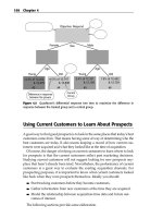
Figure 4.5 Quadstone’s differential response tree tries to maximize the difference in
response between the treated group and a control group.
Using Current Customers to Learn About Prospects
A good way to find good prospects is to look in the same places that today’s best
customers came from. That means having some of way of determining who the
best customers are today. It also means keeping a record of how current cus-
tomers were acquired and what they looked like at the time of acquisition.
Of course, the danger of relying on current customers to learn where to look
for prospects is that the current customers reflect past marketing decisions.
Studying current customers will not suggest looking for new prospects any-
place that hasn’t already been tried. Nevertheless, the performance of current
customers is a great way to evaluate the existing acquisition channels. For
prospecting purposes, it is important to know what current customers looked
like back when they were prospects themselves. Ideally you should:
■■ Start tracking customers before they become customers.
■■ Gather information from new customers at the time they are acquired.
■■ Model the relationship between acquisition-time data and future out-
comes of interest.
The following sections provide some elaboration.
470643 c04.qxd 3/8/04 11:10 AM Page 109
Data Mining Applications 109

Start Tracking Customers before
They Become Customers
It is a good idea to start recording information about prospects even before
they become customers. Web sites can accomplish this by issuing a cookie each
time a visitor is seen for the first time and starting an anonymous profile that
remembers what the visitor did. When the visitor returns (using the same
browser on the same computer), the cookie is recognized and the profile is
updated. When the visitor eventually becomes a customer or registered user,
the activity that led up to that transition becomes part of the customer record.
Tracking responses and responders is good practice in the offline world as
well. The first critical piece of information to record is the fact that the prospect
responded at all. Data describing who responded and who did not is a necessary
ingredient of future response models. Whenever possible, the response data
should also include the marketing action that stimulated the response, the chan-
nel through which the response was captured, and when the response came in.
Determining which of many marketing messages stimulated the response
can be tricky. In some cases, it may not even be possible. To make the job eas-
ier, response forms and catalogs include identifying codes. Web site visits cap-
ture the referring link. Even advertising campaigns can be distinguished by
using different telephone numbers, post office boxes, or Web addresses.
Depending on the nature of the product or service, responders may be
required to provide additional information on an application or enrollment
form. If the service involves an extension of credit, credit bureau information
may be requested. Information collected at the beginning of the customer rela-
tionship ranges from nothing at all to the complete medical examination some-
times required for a life insurance policy. Most companies are somewhere in
between.
Gather Information from New Customers
When a prospect first becomes a customer, there is a golden opportunity to
gather more information. Before the transformation from prospect to cus-

tomer, any data about prospects tends to be geographic and demographic.
Purchased lists are unlikely to provide anything beyond name, contact infor-
mation, and list source. When an address is available, it is possible to infer
other things about prospects based on characteristics of their neighborhoods.
Name and address together can be used to purchase household-level informa-
tion about prospects from providers of marketing data. This sort of data is use-
ful for targeting broad, general segments such as “young mothers” or “urban
teenagers” but is not detailed enough to form the basis of an individualized
customer relationship.
470643 c04.qxd 3/8/04 11:10 AM Page 110
110 Chapter 4
Among the most useful fields that can be collected for future data mining
are the initial purchase date, initial acquisition channel, offer responded to, ini-
tial product, initial credit score, time to respond, and geographic location. We
have found these fields to be predictive a wide range of outcomes of interest
such as expected duration of the relationship, bad debt, and additional
purchases. These initial values should be maintained as is, rather than being
overwritten with new values as the customer relationship develops.
Acquisition-Time Variables Can Predict Future Outcomes
By recording everything that was known about a customer at the time of
acquisition and then tracking customers over time, businesses can use data
mining to relate acquisition-time variables to future outcomes such as cus-
tomer longevity, customer value, and default risk. This information can then
be used to guide marketing efforts by focusing on the channels and messages
that produce the best results. For example, the survival analysis techniques
described in Chapter 12 can be used to establish the mean customer lifetime
for each channel. It is not uncommon to discover that some channels yield cus-
tomers that last twice as long as the customers from other channels. Assuming
that a customer’s value per month can be estimated, this translates into an
actual dollar figure for how much more valuable a typical channel A customer

is than a typical channel B customer—a figure that is as valuable as the cost-
per-response measures often used to rate channels.
Data Mining for Customer Relationship
Management
Customer relationship management naturally focuses on established cus-
tomers. Happily, established customers are the richest source of data for min-
ing. Best of all, the data generated by established customers reflects their
actual individual behavior. Does the customer pay bills on time? Check or
credit card? When was the last purchase? What product was purchased? How
much did it cost? How many times has the customer called customer service?
How many times have we called the customer? What shipping method does
the customer use most often? How many times has the customer returned a
purchase? This kind of behavioral data can be used to evaluate customers’
potential value, assess the risk that they will end the relationship, assess the
risk that they will stop paying their bills, and anticipate their future needs.
Matching Campaigns to Customers
The same response model scores that are used to optimize the budget for a
mailing to prospects are even more useful with existing customers where they
470643 c04.qxd 3/8/04 11:10 AM Page 111
Data Mining Applications 111
can be used to tailor the mix of marketing messages that a company directs to
its existing customers. Marketing does not stop once customers have been
acquired. There are cross-sell campaigns, up-sell campaigns, usage stimula-
tion campaigns, loyalty programs, and so on. These campaigns can be thought
of as competing for access to customers.
When each campaign is considered in isolation, and all customers are given
response scores for every campaign, what typically happens is that a similar
group of customers gets high scores for many of the campaigns. Some cus-
tomers are just more responsive than others, a fact that is reflected in the model
scores. This approach leads to poor customer relationship management. The

high-scoring group is bombarded with messages and becomes irritated and
unresponsive. Meanwhile, other customers never hear from the company and
so are not encouraged to expand their relationships.
An alternative is to send a limited number of messages to each customer,
using the scores to decide which messages are most appropriate for each one.
Even a customer with low scores for every offer has higher scores for some
then others. In Mastering Data Mining (Wiley, 1999), we describe how this
system has been used to personalize a banking Web site by highlighting the
products and services most likely to be of interest to each customer based on
their banking behavior.
Segmenting the Customer Base
Customer segmentation is a popular application of data mining with estab-
lished customers. The purpose of segmentation is to tailor products, services,
and marketing messages to each segment. Customer segments have tradition-
ally been based on market research and demographics. There might be a
“young and single” segment or a “loyal entrenched segment.” The problem
with segments based on market research is that it is hard to know how to
apply them to all the customers who were not part of the survey. The problem
with customer segments based on demographics is that not all “young and
singles” or “empty nesters” actually have the tastes and product affinities
ascribed to their segment. The data mining approach is to identify behavioral
segments.
Finding Behavioral Segments
One way to find behavioral segments is to use the undirected clustering tech-
niques described in Chapter 11. This method leads to clusters of similar
customers but it may be hard to understand how these clusters relate to the
business. In Chapter 2, there is an example of a bank successfully using auto-
matic cluster detection to identify a segment of small business customers that
were good prospects for home equity credit lines. However, that was only one
of 14 clusters found and others did not have obvious marketing uses.

470643 c04.qxd 3/8/04 11:10 AM Page 112
112 Chapter 4
More typically, a business would like to perform a segmentation that places
every customer into some easily described segment. Often, these segments are
built with respect to a marketing goal such as subscription renewal or high
spending levels. Decision tree techniques described in Chapter 6 are ideal for
this sort of segmentation.
Another common case is when there are preexisting segment definition that
are based on customer behavior and the data mining challenge is to identify
patterns in the data that correspond to the segments. A good example is the
grouping of credit card customers into segments such as “high balance
revolvers” or “high volume transactors.”
One very interesting application of data mining to the task of finding pat-
terns corresponding to predefined customer segments is the system that AT&T
Long Distance uses to decide whether a phone is likely to be used for business
purposes.
AT&T views anyone in the United States who has a phone and is not already
a customer as a potential customer. For marketing purposes, they have long
maintained a list of phone numbers called the Universe List. This is as com-
plete as possible a list of U.S. phone numbers for both AT&T and non-AT&T
customers flagged as either business or residence. The original method of
obtaining non-AT&T customers was to buy directories from local phone com-
panies, and search for numbers that were not on the AT&T customer list. This
was both costly and unreliable and likely to become more so as the companies
supplying the directories competed more and more directly with AT&T. The
original way of determining whether a number was a home or business was to
call and ask.
In 1995, Corina Cortes and Daryl Pregibon, researchers at Bell Labs (then a
part of AT&T) came up with a better way. AT&T, like other phone companies,
collects call detail data on every call that traverses its network (they are legally

mandated to keep this information for a certain period of time). Many of these
calls are either made or received by noncustomers. The telephone numbers of
non-customers appear in the call detail data when they dial AT&T 800 num-
bers and when they receive calls from AT&T customers. These records can be
analyzed and scored for likelihood to be businesses based on a statistical
model of businesslike behavior derived from data generated by known busi-
nesses. This score, which AT&T calls “bizocity,” is used to determine which
services should be marketed to the prospects.
Every telephone number is scored every day. AT&T’s switches process
several hundred million calls each day, representing about 65 million distinct
phone numbers. Over the course of a month, they see over 300 million
distinct phone numbers. Each of those numbers is given a small profile that
includes the number of days since the number was last seen, the average daily
minutes of use, the average time between appearances of the number on the
network, and the bizocity score.
TEAMFLY

Team-Fly
®

470643 c04.qxd 3/8/04 11:10 AM Page 113
Data Mining Applications 113
The bizocity score is generated by a regression model that takes into account
the length of calls made and received by the number, the time of day that call-
ing peaks, and the proportion of calls the number makes to known businesses.
Each day’s new data adjusts the score. In practice, the score is a weighted aver-
age over time with the most recent data counting the most.
Bizocity can be combined with other information in order to address partic-
ular business segments. One segment of particular interest in the past is home
businesses. These are often not recognized as businesses even by the local
phone company that issued the number. A phone number with high bizocity
that is at a residential address or one that has been flagged as residential by the
local phone company is a good candidate for services aimed at people who
work at home.
Tying Market Research Segments to Behavioral Data
One of the big challenges with traditional survey-based market research is that
it provides a lot of information about a few customers. However, to use the
results of market research effectively often requires understanding the charac-

teristics of all customers. That is, market research may find interesting seg-
ments of customers. These then need to be projected onto the existing customer
base using available data. Behavioral data can be particularly useful for this;
such behavioral data is typically summarized from transaction and billing his-
tories. One requirement of the market research is that customers need to be
identified so the behavior of the market research participants is known.
Most of the directed data mining techniques discussed in this book can be
used to build a classification model to assign people to segments based on
available data. All that is needed is a training set of customers who have
already been classified. How well this works depends largely on the extent to
which the customer segments are actually supported by customer behavior.
Reducing Exposure to Credit Risk
Learning to avoid bad customers (and noticing when good customers are
about to turn bad) is as important as holding on to good customers. Most
companies whose business exposes them to consumer credit risk do credit
screening of customers as part of the acquisition process, but risk modeling
does not end once the customer has been acquired.
Predicting Who Will Default
Assessing the credit risk on existing customers is a problem for any business
that provides a service that customers pay for in arrears. There is always the
chance that some customers will receive the service and then fail to pay for it.
470643 c04.qxd 3/8/04 11:10 AM Page 114
114 Chapter 4
Nonrepayment of debt is one obvious example; newspapers subscriptions,
telephone service, gas and electricity, and cable service are among the many
services that are usually paid for only after they have been used.
Of course, customers who fail to pay for long enough are eventually cut off.
By that time they may owe large sums of money that must be written off. With
early warning from a predictive model, a company can take steps to protect
itself. These steps might include limiting access to the service or decreasing the

length of time between a payment being late and the service being cut off.
Involuntary churn, as termination of services for nonpayment is sometimes
called, can be modeled in multiple ways. Often, involuntary churn is consid-
ered as a binary outcome in some fixed amount of time, in which case tech-
niques such as logistic regression and decision trees are appropriate. Chapter
12 shows how this problem can also be viewed as a survival analysis problem,
in effect changing the question from “Will the customer fail to pay next
month?” to “How long will it be until half the customers have been lost to
involuntary churn?”
One of the big differences between voluntary churn and involuntary churn
is that involuntary churn often involves complicated business processes, as
bills go through different stages of being late. Over time, companies may
tweak the rules that guide the processes to control the amount of money that
they are owed. When looking for accurate numbers in the near term, modeling
each step in the business processes may be the best approach.
Improving Collections
Once customers have stopped paying, data mining can aid in collections.
Models are used to forecast the amount that can be collected and, in some
cases, to help choose the collection strategy. Collections is basically a type of
sales. The company tries to sell its delinquent customers on the idea of paying
its bills instead of some other bill. As with any sales campaign, some prospec-
tive payers will be more receptive to one type of message and some to another.
Determining Customer Value
Customer value calculations are quite complex and although data mining has
a role to play, customer value calculations are largely a matter of getting finan-
cial definitions right. A seemingly simple statement of customer value is the
total revenue due to the customer minus the total cost of maintaining the cus-
tomer. But how much revenue should be attributed to a customer? Is it what
he or she has spent in total to date? What he or she spent this month? What we
expect him or her to spend over the next year? How should indirect revenues

such as advertising revenue and list rental be allocated to customers?
470643 c04.qxd 3/8/04 11:10 AM Page 115
Data Mining Applications 115
Costs are even more problematic. Businesses have all sorts of costs that may
be allocated to customers in peculiar ways. Even ignoring allocated costs and
looking only at direct costs, things can still be pretty confusing. Is it fair to
blame customers for costs over which they have no control? Two Web cus-
tomers order the exact same merchandise and both are promised free delivery.
The one that lives farther from the warehouse may cost more in shipping, but
is she really a less valuable customer? What if the next order ships from a dif-
ferent location? Mobile phone service providers are faced with a similar prob-
lem. Most now advertise uniform nationwide rates. The providers’ costs are
far from uniform when they do not own the entire network. Some of the calls
travel over the company’s own network. Others travel over the networks of
competitors who charge high rates. Can the company increase customer value
by trying to discourage customers from visiting certain geographic areas?
Once all of these problems have been sorted out, and a company has agreed
on a definition of retrospective customer value, data mining comes into play in
order to estimate prospective customer value. This comes down to estimating
the revenue a customer will bring in per unit time and then estimating the cus-
tomer’s remaining lifetime. The second of these problems is the subject of
Chapter 12.
Cross-selling, Up-selling, and Making Recommendations
With existing customers, a major focus of customer relationship management
is increasing customer profitability through cross-selling and up-selling. Data
mining is used for figuring out what to offer to whom and when to offer it.
Finding the Right Time for an Offer
Charles Schwab, the investment company, discovered that customers gener-
ally open accounts with a few thousand dollars even if they have considerably
more stashed away in savings and investment accounts. Naturally, Schwab

would like to attract some of those other balances. By analyzing historical
data, they discovered that customers who transferred large balances into
investment accounts usually did so during the first few months after they
opened their first account. After a few months, there was little return on trying
to get customers to move in large balances. The window was closed. As a
results of learning this, Schwab shifted its strategy from sending a constant
stream of solicitations throughout the customer life cycle to concentrated
efforts during the first few months.
A major newspaper with both daily and Sunday subscriptions noticed a
similar pattern. If a Sunday subscriber upgrades to daily and Sunday, it usu-
ally happens early in the relationship. A customer who has been happy with
just the Sunday paper for years is much less likely to change his or her habits.
470643 c04.qxd 3/8/04 11:10 AM Page 116
116 Chapter 4
Making Recommendations
One approach to cross-selling makes use of association rules, the subject of
Chapter 9. Association rules are used to find clusters of products that usually
sell together or tend to be purchased by the same person over time. Customers
who have purchased some, but not all of the members of a cluster are good
prospects for the missing elements. This approach works for retail products
where there are many such clusters to be found, but is less effective in areas
such as financial services where there are fewer products and many customers
have a similar mix, and the mix is often determined by product bundling and
previous marketing efforts.
Retention and Churn
Customer attrition is an important issue for any company, and it is especially
important in mature industries where the initial period of exponential growth
has been left behind. Not surprisingly, churn (or, to look on the bright side,
retention) is a major application of data mining. We use the term churn as it is
generally used in the telephone industry to refer to all types of customer attri-

tion whether voluntary or involuntary; churn is a useful word because it is one
syllable and easily used as both a noun and a verb.
Recognizing Churn
One of the first challenges in modeling churn is deciding what it is and recog-
nizing when it has occurred. This is harder in some industries than in others.
At one extreme are businesses that deal in anonymous cash transactions.
When a once loyal customer deserts his regular coffee bar for another down
the block, the barista who knew the customer’s order by heart may notice,
but the fact will not be recorded in any corporate database. Even in cases
where the customer is identified by name, it may be hard to tell the difference
between a customer who has churned and one who just hasn’t been around for
a while. If a loyal Ford customer who buys a new F150 pickup every 5 years
hasn’t bought one for 6 years, can we conclude that he has defected to another
brand?
Churn is a bit easier to spot when there is a monthly billing relationship, as
with credit cards. Even there, however, attrition might be silent. A customer
stops using the credit card, but doesn’t actually cancel it. Churn is easiest to
define in subscription-based businesses, and partly for that reason, churn
modeling is most popular in these businesses. Long-distance companies,
mobile phone service providers, insurance companies, cable companies, finan-
cial services companies, Internet service providers, newspapers, magazines,
470643 c04.qxd 3/8/04 11:10 AM Page 117
Data Mining Applications 117
and some retailers all share a subscription model where customers have a for-
mal, contractual relationship which must be explicitly ended.
Why Churn Matters
Churn is important because lost customers must be replaced by new cus-
tomers, and new customers are expensive to acquire and generally generate
less revenue in the near term than established customers. This is especially
true in mature industries where the market is fairly saturated—anyone likely

to want the product or service probably already has it from somewhere, so the
main source of new customers is people leaving a competitor.
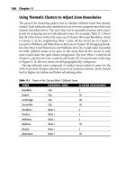
Figure 4.6 illustrates that as the market becomes saturated and the response
rate to acquisition campaigns goes down, the cost of acquiring new customers
goes up. The chart shows how much each new customer costs for a direct mail
acquisition campaign given that the mailing costs $1 and it includes an offer of
$20 in some form, such as a coupon or a reduced interest rate on a credit card.
When the response rate to the acquisition campaign is high, such as 5 percent,
the cost of a new customer is $40. (It costs $100 dollars to reach 100 people, five
of whom respond at a cost of $20 dollars each. So, five new customers cost $200
dollars.) As the response rate drops, the cost increases rapidly. By the time the
response rate drops to 1 percent, each new customer costs $200. At some point,
it makes sense to spend that money holding on to existing customers rather
than attracting new ones.
$0
$50
$100
$150
$200
$250
5.0%4.0%3.0%2.0%1.0%
Response Rate
Cost per Response
Figure 4.6 As the response rate to an acquisition campaign goes down, the cost per
customer acquired goes up.
470643 c04.qxd 3/8/04 11:10 AM Page 118
118 Chapter 4
Retention campaigns can be very effective, but also very expensive. A mobile
phone company might offer an expensive new phone to customers who renew
a contract. A credit card company might lower the interest rate. The problem

with these offers is that any customer who is made the offer will accept it. Who
wouldn’t want a free phone or a lower interest rate? That means that many of
the people accepting the offer would have remained customers even without it.
The motivation for building churn models is to figure out who is most at risk
for attrition so as to make the retention offers to high-value customers who
might leave without the extra incentive.
Different Kinds of Churn
Actually, the discussion of why churn matters assumes that churn is voluntary.
Customers, of their own free will, decide to take their business elsewhere. This
type of attrition, known as voluntary churn, is actually only one of three possi-
bilities. The other two are involuntary churn and expected churn.
Involuntary churn, also known as forced attrition, occurs when the company,
rather than the customer, terminates the relationship—most commonly due to
unpaid bills. Expected churn occurs when the customer is no longer in the tar-
get market for a product. Babies get teeth and no longer need baby food. Work-
ers retire and no longer need retirement savings accounts. Families move away
and no longer need their old local newspaper delivered to their door.
It is important not to confuse the different types of churn, but easy to do so.
Consider two mobile phone customers in identical financial circumstances.
Due to some misfortune, neither can afford the mobile phone service any
more. Both call up to cancel. One reaches a customer service agent and is
recorded as voluntary churn. The other hangs up after ten minutes on hold
and continues to use the phone without paying the bill. The second customer
is recorded as forced churn. The underlying problem—lack of money—is the
same for both customers, so it is likely that they will both get similar scores.
The model cannot predict the difference in hold times experienced by the two
subscribers.
Companies that mistake forced churn for voluntary churn lose twice—once
when they spend money trying to retain customers who later go bad and again
in increased write-offs.

Predicting forced churn can also be dangerous. Because the treatment given
to customers who are not likely to pay their bills tends to be nasty—phone ser-
vice is suspended, late fees are increased, dunning letters are sent more
quickly. These remedies may alienate otherwise good customers and increase
the chance that they will churn voluntarily.
In many companies, voluntary churn and involuntary churn are the respon-
sibilities of different groups. Marketing is concerned with holding on to good
customers and finance is concerned with reducing exposure to bad customers.
470643 c04.qxd 3/8/04 11:10 AM Page 119
Data Mining Applications 119
From a data mining point of view, it is better to address both voluntary and
involuntary churn together since all customers are at risk for both kinds of
churn to varying degrees.
Different Kinds of Churn Model
There are two basic approaches to modeling churn. The first treats churn as a
binary outcome and predicts which customers will leave and which will stay.
The second tries to estimate the customers’ remaining lifetime.
Predicting Who Will Leave
To model churn as a binary outcome, it is necessary to pick some time horizon.
If the question is “Who will leave tomorrow?” the answer is hardly anyone. If
the question is “Who will have left in 100 years?” the answer, in most busi-
nesses, is nearly everyone. Binary outcome churn models usually have a fairly
short time horizon such as 60 or 90 days. Of course, the horizon cannot be too
short or there will be no time to act on the model’s predictions.
Binary outcome churn models can be built with any of the usual tools for
classification including logistic regression, decision trees, and neural networks.
Historical data describing a customer population at one time is combined with
a flag showing whether the customers were still active at some later time. The
modeling task is to discriminate between those who left and those who stayed.
The outcome of a binary churn model is typically a score that can be used to

rank customers in order of their likelihood of churning. The most natural score
is simply the probability that the customer will leave within the time horizon
used for the model. Those with voluntary churn scores above a certain thresh-
old can be included in a retention program. Those with involuntary churn
scores above a certain threshold can be placed on a watch list.
Typically, the predictors of churn turn out to be a mixture of things that were
known about the customer at acquisition time, such as the acquisition channel
and initial credit class, and things that occurred during the customer relation-
ship such as problems with service, late payments, and unexpectedly high or
low bills. The first class of churn drivers provides information on how to lower
future churn by acquiring fewer churn-prone customers. The second class of
churn drivers provides insight into how to reduce the churn risk for customers
who are already present.
Predicting How Long Customers Will Stay
The second approach to churn modeling is the less common method, although
it has some attractive features. In this approach, the goal is to figure out
how much longer a customer is likely to stay. This approach provides more
470643 c04.qxd 3/8/04 11:10 AM Page 120
120 Chapter 4
information than simply whether the customer is expected to leave within 90
days. Having an estimate of remaining customer tenure is a necessary ingredi-
ent for a customer lifetime value model. It can also be the basis for a customer
loyalty score that defines a loyal customer as one who will remain for a long
time in the future rather than one who has remained a long time up until now.
One approach to modeling customer longevity would be to take a snapshot
of the current customer population, along with data on what these customers
looked like when they were first acquired, and try to estimate customer tenure
directly by trying to determine what long-lived customers have in common
besides an early acquisition date. The problem with this approach, is that the
longer customers have been around, the more different market conditions were

back when they were acquired. Certainly it is not safe to assume that the char-
acteristics of someone who got a cellular subscription in 1990 are good predic-
tors of which of today’s new customers will keep their service for many years.
A better approach is to use survival analysis techniques that have been bor-
rowed and adapted from statistics. These techniques are associated with the
medical world where they are used to study patient survival rates after med-
ical interventions and the manufacturing world where they are used to study
the expected time to failure of manufactured components.
Survival analysis is explained in Chapter 12. The basic idea is to calculate for
each customer (or for each group of customers that share the same values for
model input variables such as geography, credit class, and acquisition chan-
nel) the probability that having made it as far as today, he or she will leave
before tomorrow. For any one tenure this hazard, as it is called, is quite small,
but it is higher for some tenures than for others. The chance that a customer
will survive to reach some more distant future date can be calculated from the
intervening hazards.
Lessons Learned
The data mining techniques described in this book have applications in fields
as diverse as biotechnology research and manufacturing process control. This
book, however, is written for people who, like the authors, will be applying
these techniques to the kinds of business problems that arise in marketing
and customer relationship management. In most of the book, the focus on
customer-centric applications is implicit in the choice of examples used to
illustrate the techniques. In this chapter, that focus is more explicit.
Data mining is used in support of both advertising and direct marketing to
identify the right audience, choose the best communications channels, and
pick the most appropriate messages. Prospective customers can be compared
to a profile of the intended audience and given a fitness score. Should infor-
mation on individual prospects not be available, the same method can be used
470643 c04.qxd 3/8/04 11:10 AM Page 121

Data Mining Applications 121
to assign fitness scores to geographic neighborhoods using data of the type
available form the U.S. census bureau, Statistics Canada, and similar official
sources in many countries.
A common application of data mining in direct modeling is response mod-
eling. A response model scores prospects on their likelihood to respond to a
direct marketing campaign. This information can be used to improve the
response rate of a campaign, but is not, by itself, enough to determine cam-
paign profitability. Estimating campaign profitability requires reliance on esti-
mates of the underlying response rate to a future campaign, estimates of
average order sizes associated with the response, and cost estimates for fulfill-
ment and for the campaign itself. A more customer-centric use of response
scores is to choose the best campaign for each customer from among a number
of competing campaigns. This approach avoids the usual problem of indepen-
dent, score-based campaigns, which tend to pick the same people every time.
It is important to distinguish between the ability of a model to recognize
people who are interested in a product or service and its ability to recognize
people who are moved to make a purchase based on a particular campaign or
offer. Differential response analysis offers a way to identify the market seg-
ments where a campaign will have the greatest impact. Differential response
models seek to maximize the difference in response between a treated group
and a control group rather than trying to maximize the response itself.
Information about current customers can be used to identify likely prospects
by finding predictors of desired outcomes in the information that was known
about current customers before they became customers. This sort of analysis is
valuable for selecting acquisition channels and contact strategies as well as for
screening prospect lists. Companies can increase the value of their customer
data by beginning to track customers from their first response, even before they
become customers, and gathering and storing additional information when
customers are acquired.

Once customers have been acquired, the focus shifts to customer relation-
ship management. The data available for active customers is richer than that
available for prospects and, because it is behavioral in nature rather than sim-
ply geographic and demographic, it is more predictive. Data mining is used to
identify additional products and services that should be offered to customers
based on their current usage patterns. It can also suggest the best time to make
a cross-sell or up-sell offer.
One of the goals of a customer relationship management program is to
retain valuable customers. Data mining can help identify which customers are
the most valuable and evaluate the risk of voluntary or involuntary churn
associated with each customer. Armed with this information, companies can
target retention offers at customers who are both valuable and at risk, and take
steps to protect themselves from customers who are likely to default.
470643 c04.qxd 3/8/04 11:10 AM Page 122
122 Chapter 4
From a data mining perspective, churn modeling can be approached as
either a binary-outcome prediction problem or through survival analysis.
There are advantages and disadvantages to both approaches. The binary out-
come approach works well for a short horizon, while the survival analysis
approach can be used to make forecasts far into the future and provides insight
into customer loyalty and customer value as well.
TEAMFLY

Team-Fly
®

470643 c05.qxd 3/8/04 11:11 AM Page 123
5
The Lure of Statistics: Data
Mining Using Familiar Tools
CHAPTER
For statisticians (and economists too), the term “data mining” has long had a
pejorative meaning. Instead of finding useful patterns in large volumes of
data, data mining has the connotation of searching for data to fit preconceived
ideas. This is much like what politicians do around election time—search for
data to show the success of their deeds; this is certainly not what we mean by
data mining! This chapter is intended to bridge some of the gap between sta-
tisticians and data miners.

The two disciplines are very similar. Statisticians and data miners com-
monly use many of the same techniques, and statistical software vendors now
include many of the techniques described in the next eight chapters in their
software packages. Statistics developed as a discipline separate from mathe-
matics over the past century and a half to help scientists make sense of obser-
vations and to design experiments that yield the reproducible and accurate
results we associate with the scientific method. For almost all of this period,
the issue was not too much data, but too little. Scientists had to figure out
how to understand the world using data collected by hand in notebooks.
These quantities were sometimes mistakenly recorded, illegible due to fading
and smudged ink, and so on. Early statisticians were practical people who
invented techniques to handle whatever problem was at hand. Statisticians are
still practical people who use modern techniques as well as the tried and true.
123
470643 c05.qxd 3/8/04 11:11 AM Page 124
124 Chapter 5
What is remarkable and a testament to the founders of modern statistics is
that techniques developed on tiny amounts of data have survived and still
prove their utility. These techniques have proven their worth not only in the
original domains but also in virtually all areas where data is collected, from
agriculture to psychology to astronomy and even to business.
Perhaps the greatest statistician of the twentieth century was R. A. Fisher,
considered by many to be the father of modern statistics. In the 1920s, before
the invention of modern computers, he devised methods for designing and
analyzing experiments. For two years, while living on a farm outside London,
he collected various measurements of crop yields along with potential
explanatory variables—amount of rain and sun and fertilizer, for instance. To
understand what has an effect on crop yields, he invented new techniques
(such as analysis of variance—ANOVA) and performed perhaps a million cal-
culations on the data he collected. Although twenty-first-century computer

chips easily handle many millions of calculations in a second, each of Fisher’s
calculations required pulling a lever on a manual calculating machine. Results
trickled in slowly over weeks and months, along with sore hands and calluses.
The advent of computing power has clearly simplified some aspects of
analysis, although its bigger effect is probably the wealth of data produced. Our
goal is no longer to extract every last iota of possible information from each rare
datum. Our goal is instead to make sense of quantities of data so large that they
are beyond the ability of our brains to comprehend in their raw format.
The purpose of this chapter is to present some key ideas from statistics that
have proven to be useful tools for data mining. This is intended to be neither a
thorough nor a comprehensive introduction to statistics; rather, it is an intro-
duction to a handful of useful statistical techniques and ideas. These tools are
shown by demonstration, rather than through mathematical proof.
The chapter starts with an introduction to what is probably the most impor-
tant aspect of applied statistics—the skeptical attitude. It then discusses looking
at data through a statistician’s eye, introducing important concepts and termi-
nology along the way. Sprinkled through the chapter are examples, especially
for confidence intervals and the chi-square test. The final example, using the chi-
square test to understand geography and channel, is an unusual application of
the ideas presented in the chapter. The chapter ends with a brief discussion of
some of the differences between data miners and statisticians—differences in
attitude that are more a matter of degree than of substance.
Occam’s Razor
William of Occam was a Franciscan monk born in a small English town in
1280—not only before modern statistics was invented, but also before the Renais-
sance and the printing press. He was an influential philosopher, theologian,
470643 c05.qxd 3/8/04 11:11 AM Page 125
The Lure of Statistics: Data Mining Using Familiar Tools 125
and professor who expounded many ideas about many things, including church
politics. As a monk, he was an ascetic who took his vow of poverty very seri-

ously. He was also a fervent advocate of the power of reason, denying the
existence of universal truths and espousing a modern philosophy that was
quite different from the views of most of his contemporaries living in the
Middle Ages.
What does William of Occam have to do with data mining? His name has
become associated with a very simple idea. He himself explained it in Latin
(the language of learning, even among the English, at the time), “Entia non sunt
multiplicanda sine necessitate.” In more familiar English, we would say “the sim-
pler explanation is the preferable one” or, more colloquially, “Keep it simple,
stupid.” Any explanation should strive to reduce the number of causes to a
bare minimum. This line of reasoning is referred to as Occam’s Razor and is
William of Occam’s gift to data analysis.
The story of William of Occam had an interesting ending. Perhaps because
of his focus on the power of reason, he also believed that the powers of the
church should be separate from the powers of the state—that the church
should be confined to religious matters. This resulted in his opposition to the
meddling of Pope John XXII in politics and eventually to his own excommuni-
cation. He eventually died in Munich during an outbreak of the plague in
1349, leaving a legacy of clear and critical thinking for future generations.
The Null Hypothesis
Occam’s Razor is very important for data mining and statistics, although sta-
tistics expresses the idea a bit differently. The null hypothesis is the assumption
that differences among observations are due simply to chance. To give an
example, consider a presidential poll that gives Candidate A 45 percent and
Candidate B 47 percent. Because this data is from a poll, there are several
sources of error, so the values are only approximate estimates of the popular-
ity of each candidate. The layperson is inclined to ask, “Are these two values
different?” The statistician phrases the question slightly differently, “What is
the probability that these two values are really the same?”
Although the two questions are very similar, the statistician’s has a bit of an

attitude. This attitude is that the difference may have no significance at all and
is an example of using the null hypothesis. There is an observed difference of
2 percent in this example. However, this observed value may be explained by
the particular sample of people who responded. Another sample may have a
difference of 2 percent in the other direction, or may have a difference of 0 per-
cent. All are reasonably likely results from a poll. Of course, if the preferences
differed by 20 percent, then sampling variation is much less likely to be the
cause. Such a large difference would greatly improve the confidence that one
candidate is doing better than the other, and greatly reduce the probability of
the null hypothesis being true.
470643 c05.qxd 3/8/04 11:11 AM Page 126
126 Chapter 5
TIP The simplest explanation is usually the best one—even (or especially) if it
does not prove the hypothesis you want to prove.
This skeptical attitude is very valuable for both statisticians and data min-
ers. Our goal is to demonstrate results that work, and to discount the null
hypothesis. One difference between data miners and statisticians is that data
miners are often working with sufficiently large amounts of data that make it
unnecessary to worry about the mechanics of calculating the probability of
something being due to chance.
P-Values
The null hypothesis is not merely an approach to analysis; it can also be quan-
tified. The p-value is the probability that the null hypothesis is true. Remember,
when the null hypothesis is true, nothing is really happening, because differ-
ences are due to chance. Much of statistics is devoted to determining bounds
for the p-value.
Consider the previous example of the presidential poll. Consider that the
p-value is calculated to be 60 percent (more on how this is done later in the
chapter). This means that there is a 60 percent likelihood that the difference in
the support for the two candidates as measured by the poll is due strictly to

chance and not to the overall support in the general population. In this case,
there is little evidence that the support for the two candidates is different.
Let’s say the p-value is 5 percent, instead. This is a relatively small number,
and it means that we are 95 percent confident that Candidate B is doing better
than Candidate A. Confidence, sometimes called the q-value, is the flip side of
the p-value. Generally, the goal is to aim for a confidence level of at least 90
percent, if not 95 percent or more (meaning that the corresponding p-value is
less than 10 percent, or 5 percent, respectively).
These ideas—null hypothesis, p-value, and confidence—are three basic
ideas in statistics. The next section carries these ideas further and introduces
the statistical concept of distributions, with particular attention to the normal
distribution.
A Look at Data
A statistic refers to a measure taken on a sample of data. Statistics is the study
of these measures and the samples they are measured on. A good place to start,
then, is with such useful measures, and how to look at data.
470643 c05.qxd 3/8/04 11:11 AM Page 127
The Lure of Statistics: Data Mining Using Familiar Tools 127
Looking at Discrete Values
Much of the data used in data mining is discrete by nature, rather than contin-
uous. Discrete data shows up in the form of products, channels, regions, and
descriptive information about businesses. This section discusses ways of look-
ing at and analyzing discrete fields.
Histograms
The most basic descriptive statistic about discrete fields is the number of
times different values occur. Figure 5.1 shows a histogram of stop reason codes
during a period of time. A histogram shows how often each value occurs in the
data and can have either absolute quantities (204 times) or percentage (14.6
percent). Often, there are too many values to show in a single histogram such
as this case where there are over 30 additional codes grouped into the “other”

category.
In addition to the values for each category, this histogram also shows the
cumulative proportion of stops, whose scale is shown on the left-hand side.
Through the cumulative histogram, it is possible to see that the top three codes
account for about 50 percent of stops, and the top 10, almost 90 percent. As an
aesthetic note, the grid lines intersect both the left- and right-hand scales at
sensible points, making it easier to read values off of the chart.
10,048
5,944
3,851
3,549
3,311
3,054
1,491
1,306
1,226
1,108
4,884
0
2,500
5,000
7,500
10,000
12,500
TI NO VN PE CM CP NR MV EX
Stop Reason Code
Number of Stops
0%
20%
40%

60%
80%
100%
OT OTHER
Cumulative Proportion
Figure 5.1 This example shows both a histogram (as a vertical bar chart) and cumulative
proportion (as a line) on the same chart for stop reasons associated with a particular
marketing effort.
470643 c05.qxd 3/8/04 11:11 AM Page 128
128 Chapter 5
Time Series
Histograms are quite useful and easily made with Excel or any statistics pack-
age. However, histograms describe a single moment. Data mining is often
concerned with what is happening over time. A key question is whether the
frequency of values is constant over time.
Time series analysis requires choosing an appropriate time frame for the
data; this includes not only the units of time, but also when we start counting
from. Some different time frames are the beginning of a customer relationship,
when a customer requests a stop, the actual stop date, and so on. Different
fields belong in different time frames. For example:
■■ Fields describing the beginning of a customer relationship—such as
original product, original channel, or original market—should be
looked at by the customer’s original start date.
■■ Fields describing the end of a customer relationship—such as last
product, stop reason, or stop channel—should be looked at by the cus-
tomer’s stop date or the customer’s tenure at that point in time.
■■ Fields describing events during the customer relationship—such as
product upgrade or downgrade, response to a promotion, or a late
payment—should be looked at by the date of the event, the customer’s
tenure at that point in time, or the relative time since some other event.

The next step is to plot the time series as shown in Figure 5.2. This figure has
two series for stops by stop date. One shows a particular stop type over time
(price increase stops) and the other, the total number of stops. Notice that the
units for the time axis are in days. Although much business reporting is done
at the weekly and monthly level, we prefer to look at data by day in order to
see important patterns that might emerge at a fine level of granularity, patterns
that might be obscured by summarization. In this case, there is a clear up and
down wiggling pattern in both lines. This is due to a weekly cycle in stops. In
addition, the lighter line is for the price increase related stops. These clearly
show a marked increase starting in February, due to a change in pricing.
TIP When looking at field values over time, look at the data by day to get a
feel for the data at the most granular level.
A time series chart has a wealth of information. For example, fitting a line to
the data makes it possible to see and quantify long term trends, as shown in
Figure 5.2. Be careful when doing this, because of seasonality. Partial years
might introduce inadvertent trends, so include entire years when using a best-
fit line. The trend in this figure shows an increase in stops. This may be nothing
to worry about, especially since the number of customers is also increasing
over this period of time. This suggests that a better measure would be the stop
rate, rather than the raw number of stops.
470643 c05.qxd 3/8/04 11:11 AM Page 129
The Lure of Statistics: Data Mining Using Familiar Tools 129
Sep Oct Dec Mar Apr
increasing trend in
May Jun Jul Aug Nov Jan Feb May Jun
overall stops by day
price complaint stops
best fit line shows
overall stops
Figure 5.2 This chart shows two time series plotted with different scales. The dark line is

for overall stops; the light line for pricing related stops shows the impact of a change in
pricing strategy at the end of January.
Standardized Values
A time series chart provides useful information. However, it does not give an
idea as to whether the changes over time are expected or unexpected. For this,
we need some tools from statistics.
One way of looking at a time series is as a partition of all the data, with a little
bit on each day. The statistician now wants to ask a skeptical question: “Is it pos-
sible that the differences seen on each day are strictly due to chance?” This is the
null hypothesis, which is answered by calculating the p-value—the probability
that the variation among values could be explained by chance alone.
Statisticians have been studying this fundamental question for over a cen-
tury. Fortunately, they have also devised some techniques for answering it.
This is a question about sample variation. Each day represents a sample of
stops from all the stops that occurred during the period. The variation in stops
observed on different days might simply be due to an expected variation in
taking random samples.
There is a basic theorem in statistics, called the Central Limit Theorem,
which says the following:
As more and more samples are taken from a population, the distribution of the
averages of the samples (or a similar statistic) follows the normal distribution.
The average (what statisticians call the mean) of the samples comes arbitrarily
close to the average of the entire population.
470643 c05.qxd 3/8/04 11:11 AM Page 130
130 Chapter 5
The Central Limit Theorem is actually a very deep theorem and quite inter-
esting. More importantly, it is useful. In the case of discrete variables, such as
number of customers who stop on each day, the same idea holds. The statistic
used for this example is the count of the number of stops on each day, as
shown earlier in Figure 5.2. (Strictly speaking, it would be better to use a pro-

portion, such as the ratio of stops to the number of customers; this is equiva-
lent to the count for our purposes with the assumption that the number of
customers is constant over the period.)
The normal distribution is described by two parameters, the mean and the
standard deviation. The mean is the average count for each day. The standard
deviation is a measure of the extent to which values tend to cluster around the
mean and is explained more fully later in the chapter; for now, using a function
such as STDEV() in Excel or STDDEV() in SQL is sufficient. For the time series,
the standard deviation is the standard deviation of the daily counts. Assuming
that the values for each day were taken randomly from the stops for the entire
period, the set of counts should follow a normal distribution. If they don’t
follow a normal distribution, then something besides chance is affecting the
values. Notice that this does not tell us what is affecting the values, only that
the simplest explanation, sample variation, is insufficient to explain them.
This is the motivation for standardizing time series values. This process pro-
duces the number of standard deviations from the average:
■■ Calculate the average value for all days.
■■ Calculate the standard deviation for all days.
■■ For each value, subtract the average and divide by the standard deviation
to get the number of standard deviations from the average.
The purpose of standardizing the values is to test the null hypothesis. When
true, the standardized values should follow the normal distribution (with an
average of 0 and a standard deviation of 1), exhibiting several useful proper-
ties. First, the standardized value should take on negative values and positive
values with about equal frequency. Also, when standardized, about two-thirds
(68.4 percent) of the values should be between minus one and one. A bit over
95 percent of the values should be between –2 and 2. And values over 3 or less
than –3 should be very, very rare—probably not visible in the data. Of course,
“should” here means that the values are following the normal distribution and
the null hypothesis holds (that is, all time related effects are explained by sam-

ple variation). When the null hypothesis does not hold, it is often apparent
from the standardized values. The aside, “A Question of Terminology,” talks a
bit more about distributions, normal and otherwise.
Figure 5.3 shows the standardized values for the data in Figure 5.2. The first
thing to notice is that the shape of the standardized curve is very similar to the
shape of the original data; what has changed is the scale on the vertical dimen-
sion. When comparing two curves, the scales for each change. In the previous
470643 c05.qxd 3/8/04 11:11 AM Page 131
The Lure of Statistics: Data Mining Using Familiar Tools 131
figure, overall stops were much larger than pricing stops, so the two were
shown using different scales. In this case, the standardized pricing stops are
towering over the standardized overall stops, even though both are on the
same scale.
The overall stops in Figure 5.3 are pretty typically normal, with the follow-
ing caveats. There is a large peak in December, which probably needs to be
explained because the value is over four standard deviations away from the
average. Also, there is a strong weekly trend. It would be a good idea to repeat
this chart using weekly stops instead of daily stops, to see the variation on the
weekly level.
The lighter line showing the pricing related stops clearly does not follow the
normal distribution. Many more values are negative than positive. The peak is
at over 13—which is way, way too high.
Standardized values, or z-values as they are often called, are quite useful. This
example has used them for looking at values over time too see whether the val-
ues look like they were taken randomly on each day; that is, whether the varia-
tion in daily values could be explained by sampling variation. On days when
the z-value is relatively high or low, then we are suspicious that something else
is at work, that there is some other factor affecting the stops. For instance, the
peak in pricing stops occurred because there was a change in pricing. The effect
is quite evident in the daily z-values.

The z-value is useful for other reasons as well. For instance, it is one way of
taking several variables and converting them to similar ranges. This can be
useful for several data mining techniques, such as clustering and neural net-
works. Other uses of the z-value are covered in Chapter 17, which discusses
data transformations.
-2
-1
0
1
2
3
4
5
6
7
8
9
10
11
12
13
14
Jul
Sep
Oct
Dec
Mar
Apr
(Z-Value)
May

Jun
Aug
Nov
Jan
Feb
May
Jun
Standard Deviations from Mean
Figure 5.3 Standardized values make it possible to compare different groups on the same
chart using the same scale; this shows overall stops and price increase related stops.
470643 c05.qxd 3/8/04 11:11 AM Page 132
132 Chapter 5
distribution would occur in a business where customers pay by credit card
the normal (sometimes called Gaussian or bell-shaped) distribution with a
distribution, the probability that the value falls between two values—for
a variable that follows a normal distribution will take on a value within one
standard deviation above the mean. Because the curve is symmetric, there is
mean, and hence 68.2% probability of being within one standard deviation
above the mean.
bell-shaped curve.
0%
5%
10%
15%
20%
25%
30%
35%
40%
-5 -4 -3 -2 -1 0 1 2 3 4 5

Z-Value
A QUESTION OF TERMINOLOGY
One very important idea in statistics is the idea of a distribution. For a discrete
variable, a distribution is a lot like a histogram—it tells how often a given value
occurs as a probability between 0 and 1. For instance, a uniform distribution
says that all values are equally represented. An example of a uniform
and the same number of customers pays with American Express, Visa, and
MasterCard.
The normal distribution, which plays a very special role in statistics, is an
example of a distribution for a continuous variable. The following figure shows
mean of 0 and a standard deviation of 1. The way to read this curve is to
look at areas between two points. For a value that follows the normal
example, between 0 and 1—is the area under the curve. For the values of 0
and 1, the probability is 34.1 percent; this means that 34.1 percent of the time
an additional 34.1% probability of being one standard deviation below the
The probability density function for the normal distribution looks like the familiar
Probability Density
TEAMFLY

Team-Fly
®