John wiley sons data mining techniques for marketing sales_6 ppt

470643 c05.qxd 3/8/04 11:11 AM Page 142
T
able 5.2
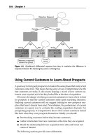
The 95 Percent Confidence Interval Bounds for the Champion Group
SEP
RESPONSE SIZE
95% CONF 95% CONF * SEP
LOWER UPPER
4.5%
900,000 0.0219% 1.96
0.0219%*1.96=0.0429% 4.46% 4.54%
4.6%
900,000 0.0221% 1.96
0.0221%*1.96=0.0433% 4.56% 4.64%
4.7%
900,000 0.0223% 1.96
0.0223%*1.96=0.0437% 4.66% 4.74%
4.8%
900,000 0.0225% 1.96
0.0225%*1.96=0.0441% 4.76% 4.84%
4.9%
900,000 0.0228% 1.96
0.0228%*1.96=0.0447% 4.86% 4.94%
5.0%
900,000 0.0230% 1.96
0.0230%*1.96=0.0451% 4.95% 5.05%
5.1%
900,000 0.0232% 1.96
0.0232%*1.96=0.0455% 5.05% 5.15%
5.2%
900,000 0.0234% 1.96

0.0234%*1.96=0.0459% 5.15% 5.25%
5.3%
900,000 0.0236% 1.96
0.0236%*1.96=0.0463% 5.25% 5.35%
5.4%
900,000 0.0238% 1.96
0.0238%*1.96=0.0466% 5.35% 5.45%
5.5%
900,000 0.0240% 1.96
0.0240%*1.96=0.0470% 5.45% 5.55%
Response rates vary from 4.5% to 5.5%. The bounds for the 95% confidence level are calculated using1.96 standard deviations fro
m the mean.
142 Chapter 5
TEAMFLY

Team-Fly
®

470643 c05.qxd 3/8/04 11:11 AM Page 143
The Lure of Statistics: Data Mining Using Familiar Tools 143
Based on these possible response rates, it is possible to tell if the confidence
bounds overlap. The 95 percent confidence bounds for the challenger model
were from about 4.86 percent to 5.14 percent. These bounds overlap the confi-
dence bounds for the champion model when its response rates are 4.9 percent,
5.0 percent, or 5.1 percent. For instance, the confidence interval for a response
rate of 4.9 percent goes from 4.86 percent to 4.94 percent; this does overlap 4.86
percent—5.14 percent. Using the overlapping bounds method, we would con-
sider these statistically the same.
Comparing Results Using Difference of Proportions
Overlapping bounds is easy but its results are a bit pessimistic. That is, even
though the confidence intervals overlap, we might still be quite confident that
the difference is not due to chance with some given level of confidence.
Another approach is to look at the difference between response rates, rather
than the rates themselves. Just as there is a formula for the standard error of a
proportion, there is a formula for the standard error of a difference of propor-
tions (SEDP):
) (p11 - p1)
SEDP =

N1 + p2 )
(1 - p2)
N2
This formula is a lot like the formula for the standard error of a proportion,
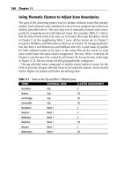
except the part in the square root is repeated for each group. Table 5.3 shows
this applied to the champion challenger problem with response rates varying
between 4.5 percent and 5.5 percent for the champion group.
By the difference of proportions, three response rates on the champion have
a confidence under 95 percent (that is, the p-value exceeds 5 percent). If the
challenger response rate is 5.0 percent and the champion is 5.1 percent, then
the difference in response rates might be due to chance. However, if the cham-
pion has a response rate of 5.2 percent, then the likelihood of the difference
being due to chance falls to under 1 percent.
WARNING Confidence intervals only measure the likelihood that sampling
affected the result. There may be many other factors that we need to take into
consideration to determine if two offers are significantly different. Each group
must be selected entirely randomly from the whole population for the
difference of proportions method to work.
470643 c05.qxd 3/8/04 11:11 AM Page 144
Table 5.3
The 95 Percent Confidence Interval Bounds for the Difference between the Champion and Challenger g
roups
CHALLE
NGER
CHAMPION
DIFFERENCE
RESPONSE SIZE
RESPONSE SIZE
VALUE SEDP Z-VALUE P-VALUE
5.0%

100,000
4.5%
900,000
0.5% 0.07% 6.9 0.0%
5.0%
100,000
4.6%
900,000
0.4% 0.07% 5.5 0.0%
5.0%
100,000
4.7%
900,000
0.3% 0.07% 4.1 0.0%
5.0%
100,000
4.8%
900,000
0.2% 0.07% 2.8 0.6%
5.0%
100,000
4.9%
900,000
0.1% 0.07% 1.4 16.8%
5.0%
100,000
5.0%
900,000
0.0% 0.07% 0.0 100.0%
5.0%

100,000
5.1%
900,000
–0.1% 0.07% –1.4 16.9%
5.0%
100,000
5.2%
900,000
–0.2% 0.07% –2.7 0.6%
5.0%
100,000
5.3%
900,000
–0.3% 0.07% –4.1 0.0%
5.0%
100,000
5.4%
900,000
–0.4% 0.07% –5.5 0.0%
5.0%
100,000
5.5%
900,000
–0.5% 0.07% –6.9 0.0%
144 Chapter 5
470643 c05.qxd 3/8/04 11:11 AM Page 145
The Lure of Statistics: Data Mining Using Familiar Tools 145
Size of Sample
The formulas for the standard error of a proportion and for the standard error
of a difference of proportions both include the sample size. There is an inverse

relationship between the sample size and the size of the confidence interval:
the larger the size of the sample, the narrower the confidence interval. So, if
you want to have more confidence in results, it pays to use larger samples.
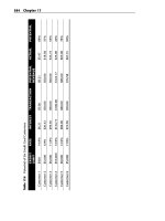
Table 5.4 shows the confidence interval for different sizes of the challenger
group, assuming the challenger response rate is observed to be 5 percent. For
very small sizes, the confidence interval is very wide, often too wide to be use-
ful. Earlier, we had said that the normal distribution is an approximation for
the estimate of the actual response rate; with small sample sizes, the estimation
is not a very good one. Statistics has several methods for handling such small
sample sizes. However, these are generally not of much interest to data miners
because our samples are much larger.
Table 5.4 The 95 Percent Confidence Interval for Difference Sizes of the Challenger Group
RESPONSE SIZE SEP 95% CONF LOWER HIGH WIDTH
5.0% 1,000 0.6892% 1.96 3.65% 6.35% 2.70%
5.0% 5,000 0.3082% 1.96 4.40% 5.60% 1.21%
5.0% 10,000 0.2179% 1.96 4.57% 5.43% 0.85%
5.0% 20,000 0.1541% 1.96 4.70% 5.30% 0.60%
5.0% 40,000 0.1090% 1.96 4.79% 5.21% 0.43%
5.0% 60,000 0.0890% 1.96 4.83% 5.17% 0.35%
5.0% 80,000 0.0771% 1.96 4.85% 5.15% 0.30%
5.0% 100,000 0.0689% 1.96 4.86% 5.14% 0.27%
5.0% 120,000 0.0629% 1.96 4.88% 5.12% 0.25%
5.0% 140,000 0.0582% 1.96 4.89% 5.11% 0.23%
5.0% 160,000 0.0545% 1.96 4.89% 5.11% 0.21%
5.0% 180,000 0.0514% 1.96 4.90% 5.10% 0.20%
5.0% 200,000 0.0487% 1.96 4.90% 5.10% 0.19%
5.0% 500,000 0.0308% 1.96 4.94% 5.06% 0.12%
5.0% 1,000,000 0.0218% 1.96 4.96% 5.04% 0.09%
470643 c05.qxd 3/8/04 11:11 AM Page 146
146 Chapter 5

What the Confidence Interval Really Means
The confidence interval is a measure of only one thing, the statistical dispersion
of the result. Assuming that everything else remains the same, it measures the
amount of inaccuracy introduced by the process of sampling. It also assumes
that the sampling process itself is random—that is, that any of the one million
customers could have been offered the challenger offer with an equal likeli-
hood. Random means random. The following are examples of what not to do:
■■ Use customers in California for the challenger and everyone else for the
champion.
■■ Use the 5 percent lowest and 5 percent highest value customers for the
challenger, and everyone else for the champion.
■■ Use the 10 percent most recent customers for the challenger, and every-
one else for the champion.
■■ Use the customers with telephone numbers for the telemarketing cam-
paign; everyone else for the direct mail campaign.
All of these are biased ways of splitting the population into groups. The pre-
vious results all assume that there is no such systematic bias. When there is
systematic bias, the formulas for the confidence intervals are not correct.
Using the formula for the confidence interval means that there is no system-
atic bias in deciding whether a particular customer receives the champion or
the challenger message. For instance, perhaps there was a champion model
that predicts the likelihood of customers responding to the champion offer. If
this model were used, then the challenger sample would no longer be a ran-
dom sample. It would consist of the leftover customers from the champion
model. This introduces another form of bias.
Or, perhaps the challenger model is only available to customers in certain
markets or with certain products. This introduces other forms of bias. In such
a case, these customers should be compared to the set of customers receiving
the champion offer with the same constraints.
Another form of bias might come from the method of response. The chal-

lenger may only accept responses via telephone, but the champion may accept
them by telephone or on the Web. In such a case, the challenger response may
be dampened because of the lack of a Web channel. Or, there might need to be
special training for the inbound telephone service reps to handle the chal-
lenger offer. At certain times, this might mean that wait times are longer,
another form of bias.
The confidence interval is simply a statement about statistics and disper-
sion. It does not address all the other forms of bias that might affect results,
and these forms of bias are often more important to results than sample varia-
tion. The next section talks about setting up a test and control experiment in
marketing, diving into these issues in more detail.
470643 c05.qxd 3/8/04 11:11 AM Page 147
The Lure of Statistics: Data Mining Using Familiar Tools 147
Size of Test and Control for an Experiment
The champion-challenger model is an example of a two-way test, where a new
method (the challenger) is compared to business-as-usual activity (the cham-
pion). This section talks about ensuring that the test and control are large
enough for the purposes at hand. The previous section talked about determin-
ing the confidence interval for the sample response rate. Here, we turn this
logic inside out. Instead of starting with the size of the groups, let’s instead
consider sizes from the perspective of test design. This requires several items
of information:
■■ Estimated response rate for one of the groups, which we call p
■■ Difference in response rates that we want to consider significant (acuity
of the test), which we call d
■■ Confidence interval (say 95 percent)
This provides enough information to determine the size of the samples
needed for the test and control. For instance, suppose that the business as
usual has a response rate of 5 percent and we want to measure with 95 percent
confidence a difference of 0.2 percent. This means that if the response of the

test group greater than 5.2 percent, then the experiment can detect the differ-
ence with a 95 percent confidence level.
For a problem of this type, the first step this is to determine the value of
SEDP. That is, if we are willing to accept a difference of 0.2 percent with a con-
fidence of 95 percent, then what is the corresponding standard error? A confi-
dence of 95 percent means that we are 1.96 standard deviations from the mean,
so the answer is to divide the difference by 1.96, which yields 0.102 percent.
More generally, the process is to convert the p-value (95 percent) to a z-value
(which can be done using the Excel function NORMSINV) and then divide the
desired confidence by this value.
The next step is to plug these values into the formula for SEDP. For this, let’s
assume that the test and control are the same size:
.%
p ) (1 - p) (1 - pd)
02
-
.
+ ( +
196
N pd )
)
N
Plugging in the values just described (p is 5% and d is 0.2%) results in:
. . .
0.102% =
5% ) 95% 5 2% ) 94 8% 0 0963
=
N
+
N N

N =
0 0963
.
=
66 875
(.
0 00102
)
2
,
So, having equal-sized groups of of 92,561 makes it possible to measure a 0.2
percent difference in response rates with a 95 percent accuracy. Of course, this
does not guarantee that the results will differ by at least 0.2 percent. It merely
470643 c05.qxd 3/8/04 11:11 AM Page 148
148 Chapter 5
says that with control and test groups of at least this size, a difference in
response rates of 0.2 percent should be measurable and statistically significant.
The size of the test and control groups affects how the results can be inter-
preted. However, this effect can be determined in advance, before the test. It is
worthwhile determining the acuity of the test and control groups before run-
ning the test, to be sure that the test can produce useful results.
TIP Before running a marketing test, determine the acuity of the test by
calculating the difference in response rates that can be measured with a high
confidence (such as 95 percent).
Multiple Comparisons
The discussion has so far used examples with only one comparison, such as
the difference between two presidential candidates or between a test and con-
trol group. Often, we are running multiple tests at the same time. For instance,
we might try out three different challenger messages to determine if one of
these produces better results than the business-as-usual message. Because

handling multiple tests does affect the underlying statistics, it is important to
understand what happens.
The Confidence Level with Multiple Comparisons
Consider that there are two groups that have been tested, and you are told that
difference between the responses in the two groups is 95 percent certain to be
due to factors other than sampling variation. A reasonable conclusion is that
there is a difference between the two groups. In a well-designed test, the most
likely reason would the difference in message, offer, or treatment.
Occam’s Razor says that we should take the simplest explanation, and not
add anything extra. The simplest hypothesis for the difference in response
rates is that the difference is not significant, that the response rates are really
approximations of the same number. If the difference is significant, then we
need to search for the reason why.
Now consider the same situation, except that you are now told that there
were actually 20 groups being tested, and you were shown only one pair. Now
you might reach a very different conclusion. If 20 groups are being tested, then
you should expect one of them to exceed the 95 percent confidence bound due
only to chance, since 95 percent means 19 times out of 20. You can no longer
conclude that the difference is due to the testing parameters. Instead, because
it is likely that the difference is due to sampling variation, this is the simplest
hypothesis.
470643 c05.qxd 3/8/04 11:11 AM Page 149
The Lure of Statistics: Data Mining Using Familiar Tools 149
The confidence level is based on only one comparison. When there are mul-
tiple comparisons, that condition is not true, so the confidence as calculated
previously is not quite sufficient.
Bonferroni’s Correction
Fortunately, there is a simple correction to fix this problem, developed by the
Italian mathematician Carlo Bonferroni. We have been looking at confidence
as saying that there is a 95 percent chance that some value is between A and B.

Consider the following situation:
■■ X is between A and B with a probability of 95 percent.
■■ Y is between C and D with a probability of 95 percent.
Bonferroni wanted to know the probability that both of these are true.
Another way to look at it is to determine the probability that one or the other
is false. This is easier to calculate. The probability that the first is false is 5 per-
cent, as is the probability of the second being false. The probability that either
is false is the sum, 10 percent, minus the probability that both are false at the
same time (0.25 percent). So, the probability that both statements are true is
about 90 percent.
Looking at this from the p-value perspective says that the p-value of both
statements together (10 percent) is approximated by the sum of the p-values of
the two statements separately. This is not a coincidence. In fact, it is reasonable
to calculate the p-value of any number of statements as the sum of the
p-values of each one. If we had eight variables with a 95 percent confidence,
then we would expect all eight to be in their ranges 60 percent at any given
time (because 8 * 5% is a p-value of 40%).
Bonferroni applied this observation in reverse. If there are eight tests and we
want an overall 95 percent confidence, then the bound for the p-value needs to
be 5% / 8 = 0.625%. That is, each observation needs to be at least 99.375 percent
confident. The Bonferroni correction is to divide the desired bound for the
p-value by the number of comparisons being made, in order to get a confi-
dence of 1 – p for all comparisons.
Chi-Square Test
The difference of proportions method is a very powerful method for estimat-
ing the effectiveness of campaigns and for other similar situations. However,
there is another statistical test that can be used. This test, the chi-square test, is
designed specifically for the situation when there are multiple tests and at least
two discrete outcomes (such as response and non-response).
470643 c05.qxd 3/8/04 11:11 AM Page 150

150 Chapter 5
The appeal of the chi-square test is that it readily adapts to multiple test
groups and multiple outcomes, so long as the different groups are distinct
from each other. This, in fact, is about the only important rule when using this
test. As described in the next chapter on decision trees, the chi-square test is
the basis for one of the earliest forms of decision trees.
Expected Values
The place to start with chi-square is to lay data out in a table, as in Table 5.5.
This is a simple 2 × 2 table, which represents a test group and a control group
in a test that has two outcomes, say response and nonresponse. This table also
shows the total values for each column and row; that is, the total number of
responders and nonresponders (each column) and the total number in the test
and control groups (each row). The response column is added for reference; it
is not part of the calculation.
What if the data were broken up between these groups in a completely unbi-
ased way? That is, what if there really were no differences between the
columns and rows in the table? This is a completely reasonable question. We
can calculate the expected values, assuming that the number of responders
and non-responders is the same, and assuming that the sizes of the champion
and challenger groups are the same. That is, we can calculate the expected
value in each cell, given that the size of the rows and columns are the same as
in the original data.
One way of calculating the expected values is to calculate the proportion of
each row that is in each column, by computing each of the following four
quantities, as shown in Table 5.6:
■■ Proportion of everyone who responds
■■ Proportion of everyone who does not respond
These proportions are then multiplied by the count for each row to obtain
the expected value. This method for calculating the expected value works
when the tabular data has more columns or more rows.

Table 5.5 The Champion-Challenger Data Laid out for the Chi-Square Test
Champion 900,000 4.80%
Challenger 5,000 95,000 5.00%
1,000,000 4.82%
RESPONDERS NON-RESPONDERS TOTAL RESPONSE
43,200 856,800
100,000
TOTAL 48,200 951,800
470643 c05.qxd 3/8/04 11:11 AM Page 151
The Lure of Statistics: Data Mining Using Familiar Tools 151
Table 5.6 Calculating the Expected Values and Deviations from Expected for the Data in
Table 5.5
EXPECTED
ACTUAL RESPONSE RESPONSE DEVIATION
YES NO TOTAL YES NO YES NO
Champion 43,200 856,800 900,000 43,380 856,620 –180 180
Challenger 5,000 95,000 100,000 4,820 95,180 180 –180
TOTAL 48,200 951,800 1,000,000 48,200 951,800
OVERALL
PROPORTION 4.82% 95.18%
The expected value is quite interesting, because it shows how the data
would break up if there were no other effects. Notice that the expected value is
measured in the same units as each cell, typically a customer count, so it actu-
ally has a meaning. Also, the sum of the expected values is the same as the sum
of all the cells in the original table. The table also includes the deviation, which
is the difference between the observed value and the expected value. In this
case, the deviations all have the same value, but with different signs. This is
because the original data has two rows and two columns. Later in the chapter
there are examples using larger tables where the deviations are different.
However, the deviations in each row and each column always cancel out, so

the sum of the deviations in each row is always 0.
Chi-Square Value
The deviation is a good tool for looking at values. However, it does not pro-
vide information as to whether the deviation is expected or not expected.
Doing this requires some more tools from statistics, namely, the chi-square dis-
tribution developed by the English statistician Karl Pearson in 1900.
The chi-square value for each cell is simply the calculation:
(x
-
expected( ))
2
x
Chi-square(x) =
expected()x
The chi-square value for the entire table is the sum of the chi-square values of
all the cells in the table. Notice that the chi-square value is always 0 or positive.
Also, when the values in the table match the expected value, then the overall
chi-square is 0. This is the best that we can do. As the deviations from the
expected value get larger in magnitude, the chi-square value also gets larger.
Unfortunately, chi-square values do not follow a normal distribution. This is
actually obvious, because the chi-square value is always positive, and the nor-
mal distribution is symmetric. The good news is that chi-square values follow
another distribution, which is also well understood. However, the chi-square
470643 c05.qxd 3/8/04 11:11 AM Page 152
152 Chapter 5
distribution depends not only on the value itself but also on the size of the table.
Figure 5.9 shows the density functions for several chi-square distributions.
What the chi-square depends on is the degrees of freedom. Unlike many
ideas in probability and statistics, degrees of freedom is easier to calculate than
to explain. The number of degrees of freedom of a table is calculated by sub-

tracting one from the number of rows and the number of columns and multi-
plying them together. The 2 × 2 table in the previous example has 1 degree of
freedom. A 5 × 7 table would have 24 (4 * 6) degrees of freedom. The aside
“Degrees of Freedom” discusses this in a bit more detail.
WARNING The chi-square test does not work when the number of expected
values in any cell is less than 5 (and we prefer a slightly higher bound).
Although this is not an issue for large data mining problems, it can be an issue
when analyzing results from a small test.
The process for using the chi-square test is:
■■ Calculate the expected values.
■■ Calculate the deviations from expected.
■■ Calculate the chi-square (square the deviations and divide by the
expected).
■■ Sum for an overall chi-square value for the table.
■■ Calculate the probability that the observed values are due to chance
(in Excel, you can use the CHIDIST function).
dof = 2
dof = 3
dof = 10
dof = 20
Probability Density
5%
4%
3%
2%
1%
0%
0 5 10 15 20 25 30 35
Chi-Square Value
Figure 5.9 The chi-square distribution depends on something called the degrees of

freedom. In general, though, it starts low, peaks early, and gradually descends.
TEAMFLY

Team-Fly
®

470643 c05.qxd 3/8/04 11:11 AM Page 153
The Lure of Statistics: Data Mining Using Familiar Tools 153

constrained the data is in the table.
If the table has r rows and c columns, then there are r * c cells in the table.
into account by subtracting the sum of the rest of values in the row from the sum
r * c – r
r * c – r – c.
the sum of all the column sums must be the same. It turns out, we have over
r * c – r – c
+ 1. Another way of writing this is ( r – 1) * (c – 1).
DEGREES OF FREEDOM
The idea behind the degrees of freedom is how many different variables are
needed to describe the table of expected values. This is a measure of how
With no constraints on the table, this is the number of variables that would be
needed. However, the calculation of the expected values has imposed some
constraints. In particular, the sum of the values in each row is the same for the
expected values as for the original table, because the sum of each row is fixed.
That is, if one value were missing, we could recalculate it by taking the constraint
for the whole row. This suggests that the degrees of freedom is . The same
situation exists for the columns, yielding an estimate of
However, there is one additional constraint. The sum of all the row sums and
counted the constraints by one, so the degrees of freedom is really
The result is the probability that the distribution of values in the table is due
to random fluctuations rather than some external criteria. As Occam’s Razor
suggests, the simplest explanation is that there is no difference at all due to the
various factors; that observed differences from expected values are entirely
within the range of expectation.
Comparison of Chi-Square to Difference of Proportions
Chi-square and difference of proportions can be applied to the same problems.
Although the results are not exactly the same, the results are similar enough
for comfort. Earlier, in Table 5.4, we determined the likelihood of champion
and challenger results being the same using the difference of proportions

method for a range of champion response rates. Table 5.7 repeats this using
the chi-square calculation instead of the difference of proportions. The
results from the chi-square test are very similar to the results from the differ-
ence of proportions—a remarkable result considering how different the two
methods are.
470643 c05.qxd 3/8/04 11:11 AM Page 154
Table 5.7
Chi-Square Calculation for Difference of Proportions Example in Table 5.4
CHALLE
NGER CHAMPION CHAL CHAMP
DIFF
CHALLENGER CHAMPION
EXP
EXP
CHI-SQUARE CHI-SQUARE CHI-SQUARE PROP
NON NON- OVERALL
NON NON NON NON
RESP RESP RESP RESP RESP
RESP RESP RESP RESP RESP RE
SP RESP RESP VALUE P-VALUE P-VALUE
5,000 95,000 40,500 859,500 4.55%
4,550 95,450 40,950 859,050 44.51 2.12 4.95 0.24 51.81 0.00% 0.00%
5,000 95,000 41,400 858,600 4.64%
4,640 95,360 41,760 858,240 27.93 1.36 3.10 0.15 32.54 0.00% 0.00%
5,000 95,000 42,300 857,700 4.73%
4,730 95,270 42,570 857,430 15.41 0.77 1.71 0.09 17.97 0.00% 0.00%
5,000 95,000 43,200 856,800 4.82%
4,820 95,180 43,380 856,620 6.72 0.34 0.75 0.04 7.85 0.51% 0.58%
5,000 95,000 44,100 855,900 4.91%
4,910 95,090 44,190 855,810 1.65 0.09 0.18 0.01 1.93 16.50% 16.83%

5,000 95,000 45,000 855,000 5.00%
5,000 95,000 45,000 855,000 0.00 0.00 0.00 0.00 0.00 100.00% 100.00%
5,000 95,000 45,900 854,100 5.09%
5,090 94,910 45,810 854,190 1.59 0.09 0.18 0.01 1.86 17.23% 16.91%
5,000 95,000 46,800 853,200 5.18%
5,180 94,820 46,620 853,380 6.25 0.34 0.69 0.04 7.33 0.68% 0.60%
5,000 95,000 47,700 852,300 5.27%
5,270 94,730 47,430 852,570 13.83 0.77 1.54 0.09 16.23 0.01% 0.00%
5,000 95,000 48,600 851,400 5.36%
5,360 94,640 48,240 851,760 24.18 1.37 2.69 0.15 28.39 0.00% 0.00%
5,000 95,000 49,500 850,500 5.45%
5,450 94,550 49,050 850,950 37.16 2.14 4.13 0.24 43.66 0.00% 0.00%
154 Chapter 5
470643 c05.qxd 3/8/04 11:11 AM Page 155
The Lure of Statistics: Data Mining Using Familiar Tools 155
An Example: Chi-Square for Regions and Starts
A large consumer-oriented company has been running acquisition campaigns
in the New York City area. The purpose of this analysis is to look at their acqui-
sition channels to try to gain an understanding of different parts of the area.
For the purposes of this analysis, three channels are of interest:
Telemarketing. Customers who are acquired through outbound telemar-
keting calls (note that this data was collected before the national do-not-
call list went into effect).
Direct mail. Customers who respond to direct mail pieces.
Other. Customers who come in through other means.
The area of interest consists of eight counties in New York State. Five of
these counties are the boroughs of New York City, two others (Nassau and Suf-
folk counties) are on Long Island, and one (Westchester) lies just north of the
city. This data was shown earlier in Table 5.1. This purpose of this analysis is to
determine whether the breakdown of starts by channel and county is due to

chance or whether some other factors might be at work.
This problem is particularly suitable for chi-square because the data can be
laid out in rows and columns, with no customer being counted in more than
one cell. Table 5.8 shows the deviation, expected values, and chi-square values
for each combination in the table. Notice that the chi-square values are often
quite large in this example. The overall chi-square score for the table is 7,200,
which is very large; the probability that the overall score is due to chance is
basically 0. That is, the variation among starts by channel and by region is not
due to sample variation. There are other factors at work.
The next step is to determine which of the values are too high and too low
and with what probability. It is tempting to convert each chi-square value in
each cell into a probability, using the degrees of freedom for the table. The
table is 8 × 3, so it has 14 degrees of freedom. However, this is not an appro-
priate thing to do. The chi-square result is for the entire table; inverting the
individual scores to get a probability does not produce valid results. Chi-
square scores are not additive.
An alternative approach proves more accurate. The idea is to compare each
cell to everything else. The result is a table that has two columns and two rows,
as shown in Table 5.9. One column is the column of the original cell; the other
column is everything else. One row is the row of the original cell; the other row
is everything else.
470643 c05.qxd 3/8/04 11:11 AM Page 156
Table 5.8
Chi-Square Calculation for Counties and Channels Example
TM
TM
TM
EXPECTED
DEVIATION
CHI-SQUARE

COUNTY
DM OTHER DM OTHER
DM OTHER
BRONX
1,850.2 523.1 4,187.7 1,362 –110 –1,252 1,002.3 23.2 374.1
KINGS
6,257.9 1,769.4 14,163.7 3,515 –376 –3,139 1,974.5 80.1 695.6
NASSAU
4,251.1 1,202.0 9,621.8 –1,116 371 745 293.0 114.5 57.7
NEW YORK 11,005.3 3,111.7 24,908.9
–3,811 –245 4,056 1,319.9 19.2 660.5
QUEENS
5,245.2 1,483.1 11,871.7 1,021 –103 –918 198.7 7.2 70.9
RICHMOND 798.9 225.9 1,808.2 –15 51 –36
0.3 11.6 0.7
SUFFOLK 3,133.6 886.0 7,092.4 –223 156
67 15.8 27.5 0.6
WESTCHESTER 3,443.8 973.7 7,794.5
–733 256 477 155.9 67.4 29.1
156 Chapter 5
470643 c05.qxd 3/8/04 11:11 AM Page 157
The Lure of Statistics: Data Mining Using Familiar Tools 157
Table 5.9 Chi-Square Calculation for Bronx and TM
TM TM TM
EXPECTED DEVIATION CHI-SQUARE
COUNTY NOT_TM NOT_TM NOT_TM
BRONX 1,850.2 4,710.8 1,361.8 –1,361.8 1,002.3 393.7
NOT BRONX 34,135.8 86,913.2 –1,361.8 1,361.8 54.3 21.3
The result is a set of chi-square values for the Bronx-TM combination, in a
table with 1 degree of freedom. The Bronx-TM score by itself is a good approx-

imation of the overall chi-square value for the 2 × 2 table (this assumes that the
original cells are roughly the same size). The calculation for the chi-square
value uses this value (1002.3) with 1 degree of freedom. Conveniently, the chi-
square calculation for this cell is the same as the chi-square for the cell in the
original calculation, although the other values do not match anything. This
makes it unnecessary to do additional calculations.
This means that an estimate of the effect of each combination of variables
can be obtained using the chi-square value in the cell with a degree of freedom
of 1. The result is a table that has a set of p-values that a given square is caused
by chance, as shown in Table 5.10.
However, there is a second correction that needs to be made because there
are many comparisons taking place at the same time. Bonferroni’s adjustment
takes care of this by multiplying each p-value by the number of comparisons—
which is the number of cells in the table. For final presentation purposes, con-
vert the p-values to their opposite, the confidence and multiply by the sign of
the deviation to get a signed confidence. Figure 5.10 illustrates the result.
Table 5.10 Estimated P-Value for Each Combination of County and Channel, without
Correcting for Number of Comparisons
COUNTY TM DM OTHER
BRONX 0.00% 0.00% 0.00%
KINGS 0.00% 0.00% 0.00%
NASSAU 0.00% 0.00% 0.00%
NEW YORK 0.00% 0.00% 0.00%
QUEENS 0.00% 0.74% 0.00%
RICHMOND 59.79% 0.07% 39.45%
SUFFOLK 0.01% 0.00% 42.91%
WESTCHESTER 0.00% 0.00% 0.00%
470643 c05.qxd 3/8/04 11:11 AM Page 158
158 Chapter 5
-100%

-80%
-60%
-40%
-20%
0%
20%
40%
60%
80%
100%
KINGS
RICHMOND
SUFFOLK
WESTCHESTER
TM
DM
BRONX
NASSAU
NEW YORK
QUEENS
OTHER
Figure 5.10 This chart shows the signed confidence values for each county and region
combination; the preponderance of values near 100% and –100% indicate that observed
differences are statistically significant.
The result is interesting. First, almost all the values are near 100 percent or
–100 percent, meaning that there are statistically significant differences among
the counties. In fact, telemarketing (the diamond) and direct mail (the square)
are always at opposite ends. There is a direct inverse relationship between the
two. Direct mail is high and telemarketing low in three counties—Manhattan,
Nassau, and Suffolk. There are many wealthy areas in these counties, suggest-

ing that wealthy customers are more likely to respond to direct mail than tele-
marketing. Of course, this could also mean that direct mail campaigns are
directed to these areas, and telemarketing to other areas, so the geography was
determined by the business operations. To determine which of these possibili-
ties is correct, we would need to know who was contacted as well as who
responded.
Data Mining and Statistics
Many of the data mining techniques discussed in the next eight chapters
were invented by statisticians or have now been integrated into statistical soft-
ware; they are extensions of standard statistics. Although data miners and
470643 c05.qxd 3/8/04 11:11 AM Page 159
The Lure of Statistics: Data Mining Using Familiar Tools 159
statisticians use similar techniques to solve similar problems, the data mining
approach differs from the standard statistical approach in several areas:
■■ Data miners tend to ignore measurement error in raw data.
■■ Data miners assume that there is more than enough data and process-
ing power.
■■ Data mining assumes dependency on time everywhere.
■■ It can be hard to design experiments in the business world.
■■ Data is truncated and censored.
These are differences of approach, rather than opposites. As such, they shed
some light on how the business problems addressed by data miners differ
from the scientific problems that spurred the development of statistics.
No Measurement Error in Basic Data
Statistics originally derived from measuring scientific quantities, such as the
width of a skull or the brightness of a star. These measurements are quantita-
tive and the precise measured value depends on factors such as the type of
measuring device and the ambient temperature. In particular, two people tak-
ing the same measurement at the same time are going to produce slightly dif-
ferent results. The results might differ by 5 percent or 0.05 percent, but there is

a difference. Traditionally, statistics looks at observed values as falling into a
confidence interval.
On the other hand, the amount of money a customer paid last January is
quite well understood—down to the last penny. The definition of customer
may be a little bit fuzzy; the definition of January may be fuzzy (consider 5-4-
4 accounting cycles). However, the amount of the payment is precise. There is
no measurement error.
There are sources of error in business data. Of particular concern is opera-
tional error, which can cause systematic bias in what is being collected. For
instance, clock skew may mean that two events that seem to happen in one
sequence may happen in another. A database record may have a Tuesday update
date, when it really was updated on Monday, because the updating process runs
just after midnight. Such forms of bias are systematic, and potentially represent
spurious patterns that might be picked up by data mining algorithms.
One major difference between business data and scientific data is that the
latter has many continuous values and the former has many discrete values.
Even monetary amounts are discrete—two values can differ only by multiples
of pennies (or some similar amount)—even though the values might be repre-
sented by real numbers.
470643 c05.qxd 3/8/04 11:11 AM Page 160
160 Chapter 5
There Is a Lot of Data
Traditionally, statistics has been applied to smallish data sets (at most a few
thousand rows) with few columns (less than a dozen). The goal has been to
squeeze as much information as possible out of the data. This is still important
in problems where collecting data is expensive or arduous—such as market
research, crash testing cars, or tests of the chemical composition of Martian soil.
Business data, on the other hand, is very voluminous. The challenge is
understanding anything about what is happening, rather than every possible
thing. Fortunately, there is also enough computing power available to handle

the large volumes of data.
Sampling theory is an important part of statistics. This area explains how
results on a subset of data (a sample) relate to the whole. This is very important
when planning to do a poll, because it is not possible to ask everyone a ques-
tion; rather, pollsters ask a very small sample and derive overall opinion.
However, this is much less important when all the data is available. Usually, it
is best to use all the data available, rather than a small subset of it.
There are a few cases when this is not necessarily true. There might simply
be too much data. Instead of building models on tens of millions of customers;
build models on hundreds of thousands—at least to learn how to build better
models. Another reason is to get an unrepresentative sample. Such a sample, for
instance, might have an equal number of churners and nonchurners, although
the original data had different proportions. However, it is generally better to
use more data rather than sample down and use less, unless there is a good
reason for sampling down.
Time Dependency Pops Up Everywhere
Almost all data used in data mining has a time dependency associated with it.
Customers’ reactions to marketing efforts change over time. Prospects’ reac-
tions to competitive offers change over time. Comparing results from a mar-
keting campaign one year to the previous year is rarely going to yield exactly
the same result. We do not expect the same results.
On the other hand, we do expect scientific experiments to yield similar results
regardless of when the experiment takes place. The laws of science are consid-
ered immutable; they do not change over time. By contrast, the business climate
changes daily. Statistics often considers repeated observations to be indepen-
dent observations. That is, one observation does not resemble another. Data
mining, on the other hand, must often consider the time component of the data.
Experimentation is Hard
Data mining has to work within the constraints of existing business practices.
This can make it difficult to set up experiments, for several reasons:

470643 c05.qxd 3/8/04 11:11 AM Page 161
The Lure of Statistics: Data Mining Using Familiar Tools 161
■■ Businesses may not be willing to invest in efforts that reduce short-term
gain for long-term learning.
■■ Business processes may interfere with well-designed experimental
methodologies.
■■ Factors that may affect the outcome of the experiment may not be
obvious.
■■ Timing plays a critical role and may render results useless.
Of these, the first two are the most difficult. The first simply says that tests
do not get done. Or, they are done so poorly that the results are useless. The
second poses the problem that a seemingly well-designed experiment may not
be executed correctly. There are always hitches when planning a test; some-
times these hitches make it impossible to read the results.
Data Is Censored and Truncated
The data used for data mining is often incomplete, in one of two special ways.
Censored values are incomplete because whatever is being measured is not
complete. One example is customer tenures. For active customers, we know
the tenure is greater than the current tenure; however, we do not know which
customers are going to stop tomorrow and which are going to stop 10 years
from now. The actual tenure is greater than the observed value and cannot be
known until the customer actually stops at some unknown point in the future.
0
5
10
15
20
25
30
35

40
45
50
0 5 10 15 20 25 30 35 40
Time
Lost Sales
Sell-Out
Demand
Inventory Units
Stock
Figure 5.11 A time series of product sales and inventory illustrates the problem of
censored data.
470643 c05.qxd 3/8/04 11:11 AM Page 162
162 Chapter 5
Figure 5.11 shows another situation with the same result. This curve shows
sales and inventory for a retailer for one product. Sales are always less than or
equal to the inventory. On the days with the Xs, though, the inventory sold
out. What were the potential sales on these days? The potential sales are
greater than or equal to the observed sales—another example of censored data.
Truncated data poses another problem in terms of biasing samples. Trun-
cated data is not included in databases, often because it is too old. For instance,
when Company A purchases Company B, their systems are merged. Often, the
active customers from Company B are moved into the data warehouse for
Company A. That is, all customers active on a given date are moved over.
Customers who had stopped the day before are not moved over. This is an
example of left truncation, and it pops up throughout corporate databases,
usually with no warning (unless the documentation is very good about saying
what is not in the warehouse as well as what is). This can cause confusion
when looking at when customers started—and discovering that all customers
who started 5 years before the merger were mysteriously active for at least 5

years. This is not due to a miraculous acquisition program. This is because all
the ones who stopped earlier were excluded.
Lessons Learned
This chapter talks about some basic statistical methods that are useful for ana-
lyzing data. When looking at data, it is useful to look at histograms and cumu-
lative histograms to see what values are most common. More important,
though, is looking at values over time.
One of the big questions addressed by statistics is whether observed values
are expected or not. For this, the number of standard deviations from the mean
(z-score) can be used to calculate the probability of the value being due to
chance (the p-value). High p-values mean that the null hypothesis is true; that
is, nothing interesting is happening. Low p-values are suggestive that other
factors may be influencing the results. Converting z-scores to p-values
depends on the normal distribution.
Business problems often require analyzing data expressed as proportions.
Fortunately, these behave similarly to normal distributions. The formula for the
standard error for proportions (SEP) makes it possible to define a confidence
interval on a proportion such as a response rate. The standard error for the dif-
ference of proportions (SEDP) makes it possible to determine whether two val-
ues are similar. This works by defining a confidence interval for the difference
between two values.
When designing marketing tests, the SEP and SEDP can be used for sizing
test and control groups. In particular, these groups should be large enough to
TEAMFLY

Team-Fly
®

470643 c05.qxd 3/8/04 11:11 AM Page 163
The Lure of Statistics: Data Mining Using Familiar Tools 163
measure differences in response with a high enough confidence. Tests that
have more than two groups need to take into account an adjustment, called
Bonferroni’s correction, when setting the group sizes.
The chi-square test is another statistical method that is often useful. This
method directly calculates the estimated values for data laid out in rows and
columns. Based on these estimates, the chi-square test can determine whether
the results are likely or unlikely. As shown in an example, the chi-square test
and SEDP methods produce similar results.

Statisticians and data miners solve similar problems. However, because of
historical differences and differences in the nature of the problems, there are
some differences in approaches. Data miners generally have lots and lots of
data with few measurement errors. This data changes over time, and values
are sometimes incomplete. The data miner has to be particularly suspicious
about bias introduced into the data by business processes.
The next eight chapters dive into more detail into more modern techniques
for building models and understanding data. Many of these techniques have
been adopted by statisticians and build on over a century of work in this area.
470643 c05.qxd 3/8/04 11:11 AM Page 164
470643 c06.qxd 3/8/04 11:12 AM Page 165
6
Decision Trees
CHAPTER
Decision trees are powerful and popular for both classification and prediction.
The attractiveness of tree-based methods is due largely to the fact that decision
trees represent rules. Rules can readily be expressed in English so that we
humans can understand them; they can also be expressed in a database access
language such as SQL to retrieve records in a particular category. Decision
trees are also useful for exploring data to gain insight into the relationships of
a large number of candidate input variables to a target variable. Because deci-
sion trees combine both data exploration and modeling, they are a powerful
first step in the modeling process even when building the final model using
some other technique.
There is often a trade-off between model accuracy and model transparency.
In some applications, the accuracy of a classification or prediction is the only
thing that matters; if a direct mail firm obtains a model that can accurately pre-
dict which members of a prospect pool are most likely to respond to a certain
solicitation, the firm may not care how or why the model works. In other situ-
ations, the ability to explain the reason for a decision is crucial. In insurance

underwriting, for example, there are legal prohibitions against discrimination
based on certain variables. An insurance company could find itself in the posi-
tion of having to demonstrate to a court of law that it has not used illegal dis-
criminatory practices in granting or denying coverage. Similarly, it is more
acceptable to both the loan officer and the credit applicant to hear that an
application for credit has been denied on the basis of a computer-generated
165
470643 c06.qxd 3/8/04 11:12 AM Page 166
166 Chapter 6
rule (such as income below some threshold and number of existing revolving
accounts greater than some other threshold) than to hear that the decision has
been made by a neural network that provides no explanation for its action.
This chapter begins with an examination of what decision trees are, how
they work, and how they can be applied to classification and prediction prob-
lems. It then describes the core algorithm used to build decision trees and dis-
cusses some of the most popular variants of that core algorithm. Practical
examples drawn from the authors’ experience are used to demonstrate the
utility and general applicability of decision tree models and to illustrate prac-
tical considerations that must be taken into account.
What Is a Decision Tree?
A decision tree is a structure that can be used to divide up a large collection of
records into successively smaller sets of records by applying a sequence of
simple decision rules. With each successive division, the members of the
resulting sets become more and more similar to one another. The familiar divi-
sion of living things into kingdoms, phyla, classes, orders, families, genera,
and species, invented by the Swedish botanist Carl Linnaeus in the 1730s, pro-
vides a good example. Within the animal kingdom, a particular animal is
assigned to the phylum chordata if it has a spinal cord. Additional characteris-
tics are used to further subdivide the chordates into the birds, mammals, rep-
tiles, and so on. These classes are further subdivided until, at the lowest level

in the taxonomy, members of the same species are not only morphologically
similar, they are capable of breeding and producing fertile offspring.
A decision tree model consists of a set of rules for dividing a large heteroge-
neous population into smaller, more homogeneous groups with respect to a
particular target variable. A decision tree may be painstakingly constructed by
hand in the manner of Linnaeus and the generations of taxonomists that fol-
lowed him, or it may be grown automatically by applying any one of several
decision tree algorithms to a model set comprised of preclassified data. This
chapter is mostly concerned with the algorithms for automatically generating
decision trees. The target variable is usually categorical and the decision tree
model is used either to calculate the probability that a given record belongs to
each of the categories, or to classify the record by assigning it to the most likely
class. Decision trees can also be used to estimate the value of a continuous
variable, although there are other techniques more suitable to that task.
Classification
Anyone familiar with the game of Twenty Questions will have no difficulty
understanding how a decision tree classifies records. In the game, one player