John wiley sons data mining techniques for marketing sales_8 ppt

470643 c06.qxd 3/8/04 11:12 AM Page 210
470643 c07.qxd 3/8/04 11:36 AM Page 211
7
Artificial Neural Networks
CHAPTER
Artificial neural networks are popular because they have a proven track record
in many data mining and decision-support applications. Neural networks—
the “artificial” is usually dropped—are a class of powerful, general-purpose
tools readily applied to prediction, classification, and clustering. They have
been applied across a broad range of industries, from predicting time series in
the financial world to diagnosing medical conditions, from identifying clus-
ters of valuable customers to identifying fraudulent credit card transactions,
from recognizing numbers written on checks to predicting the failure rates of
engines.
The most powerful neural networks are, of course, the biological kind. The
human brain makes it possible for people to generalize from experience; com-
puters, on the other hand, usually excel at following explicit instructions over
and over. The appeal of neural networks is that they bridge this gap by mod-
eling, on a digital computer, the neural connections in human brains. When
used in well-defined domains, their ability to generalize and learn from data
mimics, in some sense, our own ability to learn from experience. This ability is
useful for data mining, and it also makes neural networks an exciting area for
research, promising new and better results in the future.
There is a drawback, though. The results of training a neural network are
internal weights distributed throughout the network. These weights provide
no more insight into why the solution is valid than dissecting a human brain
explains our thought processes. Perhaps one day, sophisticated techniques for
211
470643 c07.qxd 3/8/04 11:36 AM Page 212
212 Chapter 7
probing neural networks may help provide some explanation. In the mean-

time, neural networks are best approached as black boxes with internal work-
ings as mysterious as the workings of our brains. Like the responses of the
Oracle at Delphi worshipped by the ancient Greeks, the answers produced by
neural networks are often correct. They have business value—in many cases a
more important feature than providing an explanation.
This chapter starts with a bit of history; the origins of neural networks grew
out of actual attempts to model the human brain on computers. It then dis-
cusses an early case history of using this technique for real estate appraisal,
before diving into technical details. Most of the chapter presents neural net-
works as predictive modeling tools. At the end, we see how they can be used
for undirected data mining as well. A good place to begin is, as always, at the
beginning, with a bit of history.
A Bit of History
Neural networks have an interesting history in the annals of computer science.
The original work on the functioning of neurons—biological neurons—took
place in the 1930s and 1940s, before digital computers really even existed. In
1943, Warren McCulloch, a neurophysiologist at Yale University, and Walter
Pitts, a logician, postulated a simple model to explain how biological neurons
work and published it in a paper called “A Logical Calculus Immanent in
Nervous Activity.” While their focus was on understanding the anatomy of the
brain, it turned out that this model provided inspiration for the field of artifi-
cial intelligence and would eventually provide a new approach to solving cer-
tain problems outside the realm of neurobiology.
In the 1950s, when digital computers first became available, computer
scientists implemented models called perceptrons based on the work of
McCulloch and Pitts. An example of a problem solved by these early networks
was how to balance a broom standing upright on a moving cart by controlling
the motions of the cart back and forth. As the broom starts falling to the left,
the cart learns to move to the left to keep it upright. Although there were some
limited successes with perceptrons in the laboratory, the results were disap-

pointing as a general method for solving problems.
One reason for the limited usefulness of early neural networks is that most
powerful computers of that era were less powerful than inexpensive desktop
computers today. Another reason was that these simple networks had theoreti-
cal deficiencies, as shown by Seymour Papert and Marvin Minsky (two profes-
sors at the Massachusetts Institute of Technology) in 1968. Because of these
deficiencies, the study of neural network implementations on computers
slowed down drastically during the 1970s. Then, in 1982, John Hopfield of the
California Institute of Technology invented back propagation, a way of training
neural networks that sidestepped the theoretical pitfalls of earlier approaches.
TEAMFLY

Team-Fly
®

470643 c07.qxd 3/8/04 11:36 AM Page 213
Artificial Neural Networks 213
This development sparked a renaissance in neural network research. Through
the 1980s, research moved from the labs into the commercial world, where it
has since been applied to solve both operational problems—such as detecting
fraudulent credit card transactions as they occur and recognizing numeric
amounts written on checks—and data mining challenges.
At the same time that researchers in artificial intelligence were developing
neural networks as a model of biological activity, statisticians were taking
advantage of computers to extend the capabilities of statistical methods. A
technique called logistic regression proved particularly valuable for many
types of statistical analysis. Like linear regression, logistic regression tries to fit
a curve to observed data. Instead of a line, though, it uses a function called the
logistic function. Logistic regression, and even its more familiar cousin linear
regression, can be represented as special cases of neural networks. In fact, the
entire theory of neural networks can be explained using statistical methods,
such as probability distributions, likelihoods, and so on. For expository pur-
poses, though, this chapter leans more heavily toward the biological model
than toward theoretical statistics.
Neural networks became popular in the 1980s because of a convergence of
several factors. First, computing power was readily available, especially in the
business community where data was available. Second, analysts became more
comfortable with neural networks by realizing that they are closely related to

known statistical methods. Third, there was relevant data since operational
systems in most companies had already been automated. Fourth, useful appli-
cations became more important than the holy grails of artificial intelligence.
Building tools to help people superseded the goal of building artificial people.
Because of their proven utility, neural networks are, and will continue to be,
popular tools for data mining.
Real Estate Appraisal
Neural networks have the ability to learn by example in much the same way
that human experts gain from experience. The following example applies
neural networks to solve a problem familiar to most readers—real estate
appraisal.
Why would we want to automate appraisals? Clearly, automated appraisals
could help real estate agents better match prospective buyers to prospective
homes, improving the productivity of even inexperienced agents. Another use
would be to set up kiosks or Web pages where prospective buyers could
describe the homes that they wanted—and get immediate feedback on how
much their dream homes cost.
Perhaps an unexpected application is in the secondary mortgage market.
Good, consistent appraisals are critical to assessing the risk of individual loans
and loan portfolios, because one major factor affecting default is the proportion
of the value of the property at risk. If the loan value is more than 100 percent of
the market value, the risk of default goes up considerably. Once the loan has
been made, how can the market value be calculated? For this purpose, Freddie
Mac, the Federal Home Loan Mortgage Corporation, developed a product
called Loan Prospector that does these appraisals automatically for homes
throughout the United States. Loan Prospector was originally based on neural
network technology developed by a San Diego company HNC, which has since
been merged into Fair Isaac.
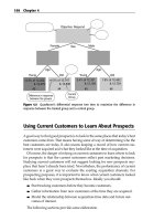
Back to the example. This neural network mimics an appraiser who
estimates the market value of a house based on features of the property (see

Figure 7.1). She knows that houses in one part of town are worth more than
those in other areas. Additional bedrooms, a larger garage, the style of the
house, and the size of the lot are other factors that figure into her mental cal-
culation. She is not applying some set formula, but balancing her experience
and knowledge of the sales prices of similar homes. And, her knowledge about
housing prices is not static. She is aware of recent sale prices for homes
throughout the region and can recognize trends in prices over time—fine-
tuning her calculation to fit the latest data.
Figure 7.1 Real estate agents and appraisers combine the features of a house to come up
with a valuation—an example of biological neural networks at work.
?
?
?
$$$
214 Chapter 7
470643 c07.qxd 3/8/04 11:36 AM Page 214
470643 c07.qxd 3/8/04 11:36 AM Page 215
Artificial Neural Networks 215
The appraiser or real estate agent is a good example of a human expert in a well-
defined domain. Houses are described by a fixed set of standard features taken
into account by the expert and turned into an appraised value. In 1992, researchers
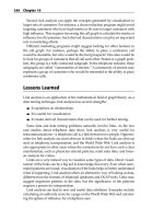
at IBM recognized this as a good problem for neural networks. Figure 7.2 illus-
trates why. A neural network takes specific inputs—in this case the information
from the housing sheet—and turns them into a specific output, an appraised value
for the house. The list of inputs is well defined because of two factors: extensive
use of the multiple listing service (MLS) to share information about the housing
market among different real estate agents and standardization of housing descrip-
tions for mortgages sold on secondary markets. The desired output is well defined
as well—a specific dollar amount. In addition, there is a wealth of experience in
the form of previous sales for teaching the network how to value a house.

Neural networks are good for prediction and estimation problems. ATIP
good problem has the following three characteristics:
■■
The inputs are well understood. You have a good idea of which features
of the data are important, but not necessarily how to combine them.
■■
The output is well understood. You know what you are trying to model.
■■
Experience is available. You have plenty of examples where both the
inputs and the output are known. These known cases are used to train
the network.
The first step in setting up a neural network to calculate estimated housing
values is determining a set of features that affect the sales price. Some possible
common features are shown in Table 7.1. In practice, these features work for
homes in a single geographical area. To extend the appraisal example to han-
dle homes in many neighborhoods, the input data would include zip code
information, neighborhood demographics, and other neighborhood quality-
of-life indicators, such as ratings of schools and proximity to transportation. To
simplify the example, these additional features are not included here.
inputs output
size of garage
living space
age of house
etc. etc. etc.
appraised value
Neural Network Model
Figure 7.2 A neural network is like a black box that knows how to process inputs to create
an output. The calculation is quite complex and difficult to understand, yet the results are
often useful.
470643 c07.qxd 3/8/04 11:36 AM Page 216

216 Chapter 7
Table 7.1 Common Features Describing a House
FEATURE DESCRIPTION RANGE OF VALUES
Num_Apartments Number of dwelling units Integer: 1–3
Year_Built Year built Integer: 1850–1986
Plumbing_Fixtures Number of plumbing fixtures Integer: 5–17
Heating_Type Heating system type coded as A or B
Basement_Garage Basement garage (number of cars) Integer: 0–2
Attached_Garage Attached frame garage area Integer: 0–228
(in square feet)
Living_Area Total living area (square feet) Integer: 714–4185
Deck_Area Deck / open porch area (square feet) Integer: 0–738
Porch_Area Enclosed porch area (square feet) Integer: 0–452
Recroom_Area Recreation room area (square feet) Integer: 0–672
Basement_Area Finished basement area (square feet) Integer: 0–810
Training the network builds a model which can then be used to estimate the
target value for unknown examples. Training presents known examples (data
from previous sales) to the network so that it can learn how to calculate the
sales price. The training examples need two more additional features: the sales
price of the home and the sales date. The sales price is needed as the target
variable. The date is used to separate the examples into a training, validation,
and test set. Table 7.2 shows an example from the training set.
The process of training the network is actually the process of adjusting
weights inside it to arrive at the best combination of weights for making the
desired predictions. The network starts with a random set of weights, so it ini-
tially performs very poorly. However, by reprocessing the training set over
and over and adjusting the internal weights each time to reduce the overall
error, the network gradually does a better and better job of approximating the
target values in the training set. When the appoximations no longer improve,
the network stops training.

470643 c07.qxd 3/8/04 11:36 AM Page 217
Artificial Neural Networks 217
Table 7.2 Sample Record from Training Set with Values Scaled to Range –1 to 1
RANGE OF ORIGINAL SCALED
FEATURE VALUES VALUE VALUE
Sales_Price $103,000–$250,000 $171,000 –0.0748
Months_Ago 0–23 4 –0.6522
Num_Apartments 1-3 1 –1.0000
Year_Built 1850–1986 1923 +0.0730
Plumbing_Fixtures 5–17 9 –0.3077
Heating_Type coded as A or B B +1.0000
Basement_Garage 0–2 0 –1.0000
Attached_Garage 0–228 120 +0.0524
Living_Area 714–4185 1,614 –0.4813
Deck_Area 0–738 0 –1.0000
Porch_Area 0–452 210 –0.0706
Recroom_Area 0–672 0 –1.0000
Basement_Area 0–810 175 –0.5672
This process of adjusting weights is sensitive to the representation of the
data going in. For instance, consider a field in the data that measures lot size.
If lot size is measured in acres, then the values might reasonably go from about
1
⁄8 to 1 acre. If measured in square feet, the same values would be 5,445 square
feet to 43,560 square feet. However, for technical reasons, neural networks
restrict their inputs to small numbers, say between –1 and 1. For instance,
when an input variable takes on very large values relative to other inputs, then
this variable dominates the calculation of the target. The neural network
wastes valuable iterations by reducing the weights on this input to lessen its
effect on the output. That is, the first “pattern” that the network will find is
that the lot size variable has much larger values than other variables. Since this

is not particularly interesting, it would be better to use the lot size as measured
in acres rather than square feet.
This idea generalizes. Usually, the inputs in the neural network should be
smallish numbers. It is a good idea to limit them to some small range, such as
–1 to 1, which requires mapping all the values, both continuous and categorical
prior to training the network.
One way to map continuous values is to turn them into fractions by sub-
tracting the middle value of the range from the value, dividing the result by the
size of the range, and multiplying by 2. For instance, to get a mapped value for
470643 c07.qxd 3/8/04 11:36 AM Page 218
218 Chapter 7
Year_Built (1923), subtract (1850 + 1986)/2 = 1918 (the middle value) from 1923
(the year the oldest house was built) and get 7. Dividing by the number of years
in the range (1986 – 1850 + 1 = 137) yields a scaled value and multiplying by 2
yields a value of 0.0730. This basic procedure can be applied to any continuous
feature to get a value between –1 and 1. One way to map categorical features is
to assign fractions between –1 and 1 to each of the categories. The only categor-
ical variable in this data is Heating_Type, so we can arbitrarily map B 1 and A to
–1. If we had three values, we could assign one to –1, another to 0, and the third
to 1, although this approach does have the drawback that the three heating
types will seem to have an order. Type –1 will appear closer to type 0 than to
type 1. Chapter 17 contains further discussion of ways to convert categorical
variables to numeric variables without adding spurious information.
With these simple techniques, it is possible to map all the fields for the sam-
ple house record shown earlier (see Table 7.2) and train the network. Training
is a process of iterating through the training set to adjust the weights. Each
iteration is sometimes called a generation.
Once the network has been trained, the performance of each generation
must be measured on the validation set. Typically, earlier generations of the
network perform better on the validation set than the final network (which

was optimized for the training set). This is due to overfitting, (which was dis-
cussed in Chapter 3) and is a consequence of neural networks being so power-
ful. In fact, neural networks are an example of a universal approximator. That
is, any function can be approximated by an appropriately complex neural
network. Neural networks and decision trees have this property; linear and
logistic regression do not, since they assume particular shapes for the under-
lying function.
As with other modeling approaches, neural networks can learn patterns that
exist only in the training set, resulting in overfitting. To find the best network
for unseen data, the training process remembers each set of weights calculated
during each generation. The final network comes from the generation that
works best on the validation set, rather than the one that works best on the
training set.
When the model’s performance on the validation set is satisfactory, the
neural network model is ready for use. It has learned from the training exam-
ples and figured out how to calculate the sales price from all the inputs. The
model takes descriptive information about a house, suitably mapped, and
produces an output. There is one caveat. The output is itself a number between
0 and 1 (for a logistic activation function) or –1 and 1 (for the hyperbolic
tangent), which needs to be remapped to the range of sale prices. For example,
the value 0.75 could be multiplied by the size of the range ($147,000) and
then added to the base number in the range ($103,000) to get an appraisal
value of $213,250.
470643 c07.qxd 3/8/04 11:36 AM Page 219
Artificial Neural Networks 219
Neural Networks for Directed Data Mining
The previous example illustrates the most common use of neural networks:
building a model for classification or prediction. The steps in this process are:
1. Identify the input and output features.
2. Transform the inputs and outputs so they are in a small range, (–1 to 1).

3. Set up a network with an appropriate topology.
4. Train the network on a representative set of training examples.
5. Use the validation set to choose the set of weights that minimizes the
error.
6. Evaluate the network using the test set to see how well it performs.
7. Apply the model generated by the network to predict outcomes for
unknown inputs.
Fortunately, data mining software now performs most of these steps auto-
matically. Although an intimate knowledge of the internal workings is not nec-
essary, there are some keys to using networks successfully. As with all
predictive modeling tools, the most important issue is choosing the right train-
ing set. The second is representing the data in such a way as to maximize
the ability of the network to recognize patterns in it. The third is interpreting
the results from the network. Finally, understanding some specific details
about how they work, such as network topology and parameters controlling
training, can help make better performing networks.
One of the dangers with any model used for prediction or classification is
that the model becomes stale as it gets older—and neural network models are
no exception to this rule. For the appraisal example, the neural network has
learned about historical patterns that allow it to predict the appraised value
from descriptions of houses based on the contents of the training set. There is
no guarantee that current market conditions match those of last week, last
month, or 6 months ago—when the training set might have been made. New
homes are bought and sold every day, creating and responding to market
forces that are not present in the training set. A rise or drop in interest rates, or
an increase in inflation, may rapidly change appraisal values. The problem of
keeping a neural network model up to date is made more difficult by two fac-
tors. First, the model does not readily express itself in the form of rules, so it
may not be obvious when it has grown stale. Second, when neural networks
degrade, they tend to degrade gracefully making the reduction in perfor-

mance less obvious. In short, the model gradually expires and it is not always
clear exactly when to update it.
470643 c07.qxd 3/8/04 11:36 AM Page 220
220 Chapter 7
The solution is to incorporate more recent data into the neural network. One
way is to take the same neural network back to training mode and start feed-
ing it new values. This is a good approach if the network only needs to tweak
results such as when the network is pretty close to being accurate, but you
think you can improve its accuracy even more by giving it more recent exam-
ples. Another approach is to start over again by adding new examples into the
training set (perhaps removing older examples) and training an entirely new
network, perhaps even with a different topology (there is further discussion of
network topologies later). This is appropriate when market conditions may
have changed drastically and the patterns found in the original training set are
no longer applicable.
The virtuous cycle of data mining described in Chapter 2 puts a premium on
measuring the results from data mining activities. These measurements help
in understanding how susceptible a given model is to aging and when a neural
network model should be retrained.
A neural network is only as good as the training set used toWARNING
generate it. The model is static and must be explicitly updated by adding more
recent examples into the training set and retraining the network (or training a
new network) in order to keep it up-to-date and useful.
What Is a Neural Net?
Neural networks consist of basic units that mimic, in a simplified fashion, the
behavior of biological neurons found in nature, whether comprising the brain
of a human or of a frog. It has been claimed, for example, that there is a unit
within the visual system of a frog that fires in response to fly-like movements,
and that there is another unit that fires in response to things about the size of a
fly. These two units are connected to a neuron that fires when the combined

value of these two inputs is high. This neuron is an input into yet another
which triggers tongue-flicking behavior.
The basic idea is that each neural unit, whether in a frog or a computer, has
many inputs that the unit combines into a single output value. In brains, these
units may be connected to specialized nerves. Computers, though, are a bit
simpler; the units are simply connected together, as shown in Figure 7.3, so the
outputs from some units are used as inputs into others. All the examples in
Figure 7.3 are examples of feed-forward neural networks, meaning there is a
one-way flow through the network from the inputs to the outputs and there
are no cycles in the network.
Figure 7.3 Feed-forward neural networks take inputs on one end and transform them into
outputs.
input 1
input 2
input 3
input 4
output
This simple neural network
takes four inputs and
produces an output. This
result of training this network
is equivalent to the statistical
technique called logistic
regression.
input 1
input 2
input 3
input 4
output
This network has a middle layer

called the
hidden layer
, which
makes the network more
powerful by enabling it to
recognize more patterns.
input 1
input 2
input 3
input 4
output
Increasing the size of the hidden
layer makes the network more
powerful but introduces the risk
of overfitting. Usually, only one
hidden layer is needed.
input 1
input 2
input 3
output 2
A neural network can produce
multiple output values.
output 1
output 3
input 4
Artificial Neural Networks 221
470643 c07.qxd 3/8/04 11:36 AM Page 221
470643 c07.qxd 3/8/04 11:36 AM Page 222
222 Chapter 7
Feed-forward networks are the simplest and most useful type of network

for directed modeling. There are three basic questions to ask about them:
■■ What are units and how do they behave? That is, what is the activation
function?
■■ How are the units connected together? That is, what is the topology of a
network?
■■ How does the network learn to recognize patterns? That is, what is
back propagation and more generally how is the network trained?
The answers to these questions provide the background for understanding
basic neural networks, an understanding that provides guidance for getting
the best results from this powerful data mining technique.
What Is the Unit of a Neural Network?
Figure 7.4 shows the important features of the artificial neuron. The unit com-
bines its inputs into a single value, which it then transforms to produce the
output; these together are called the activation function. The most common acti-
vation functions are based on the biological model where the output remains
very low until the combined inputs reach a threshold value. When the com-
bined inputs reach the threshold, the unit is activated and the output is high.
Like its biological counterpart, the unit in a neural network has the property
that small changes in the inputs, when the combined values are within some
middle range, can have relatively large effects on the output. Conversely, large
changes in the inputs may have little effect on the output, when the combined
inputs are far from the middle range. This property, where sometimes small
changes matter and sometimes they do not, is an example of nonlinear behavior.
The power and complexity of neural networks arise from their nonlinear
behavior, which in turn arises from the particular activation function used by
the constituent neural units.
The activation function has two parts. The first part is the combination func-
tion that merges all the inputs into a single value. As shown in Figure 7.4, each
input into the unit has its own weight. The most common combination func-
tion is the weighted sum, where each input is multiplied by its weight and

these products are added together. Other combination functions are some-
times useful and include the maximum of the weighted inputs, the minimum,
and the logical AND or OR of the values. Although there is a lot of flexibility
in the choice of combination functions, the standard weighted sum works well
in many situations. This element of choice is a common trait of neural net-
works. Their basic structure is quite flexible, but the defaults that correspond
to the original biological models, such as the weighted sum for the combina-
tion function, work well in practice.
TEAMFLY

Team-Fly
®

470643 c07.qxd 3/8/04 11:36 AM Page 223
Artificial Neural Networks 223
w1
w3
w2
output
{
bias
0
1
-1
The result is one output value,
usually between -1 and 1.
The
transfer function
calculates the
output value from the result of the
combination function.
The
combination function
combines
all the inputs into a single value,
usually as a weighted summation.
Each input has its own weight,
plus there is an additional

weight called the
bias.
The
combination
function
and
transfer function
together constitute
the
activation
function.
inputs
Figure 7.4 The unit of an artificial neural network is modeled on the biological neuron.
The output of the unit is a nonlinear combination of its inputs.
The second part of the activation function is the transfer function, which gets
its name from the fact that it transfers the value of the combination function to
the output of the unit. Figure 7.5 compares three typical transfer functions: the
sigmoid (logistic), linear, and hyperbolic tangent functions. The specific values
that the transfer function takes on are not as important as the general form of
the function. From our perspective, the linear transfer function is the least inter-
esting. A feed-forward neural network consisting only of units with linear
transfer functions and a weighted sum combination function is really just doing
a linear regression. Sigmoid functions are S-shaped functions, of which the two
most common for neural networks are the logistic and the hyperbolic tangent.
The major difference between them is the range of their outputs, between 0 and
1 for the logistic and between –1 and 1 for the hyperbolic tangent.
The logistic and hyperbolic tangent transfer functions behave in a similar
way. Even though they are not linear, their behavior is appealing to statisti-
cians. When the weighted sum of all the inputs is near 0, then these functions
are a close approximation of a linear function. Statisticians appreciate linear

systems, and almost-linear systems are almost as well appreciated. As the
470643 c07.qxd 3/8/04 11:36 AM Page 224
224 Chapter 7
magnitude of the weighted sum gets larger, these transfer functions gradually
saturate (to 0 and 1 in the case of the logistic; to –1 and 1 in the case of the
hyperbolic tangent). This behavior corresponds to a gradual movement from a
linear model of the input to a nonlinear model. In short, neural networks have
the ability to do a good job of modeling on three types of problems: linear
problems, near-linear problems, and nonlinear problems. There is also a rela-
tionship between the activation function and the range of input values, as dis-
cussed in the sidebar, “Sigmoid Functions and Ranges for Input Values.”
A network can contain units with different transfer functions, a subject
we’ll return to later when discussing network topology. Sophisticated tools
sometimes allow experimentation with other combination and transfer func-
tions. Other functions have significantly different behavior from the standard
units. It may be fun and even helpful to play with different types of activation
functions. If you do not want to bother, though, you can have confidence in the
standard functions that have proven successful for many neural network
applications.
1.0
0.5
0.0
-0.5
-1.0
Exponential (tanh)
0
Sigmoid
(logistic)
Linear
Figure 7.5 Three common transfer functions are the sigmoid, linear, and hyperbolic tangent

functions.
470643 c07.qxd 3/8/04 11:36 AM Page 225
Artificial Neural Networks 225
hyperbolic tangent produces values between –1 and 1 for all possible outputs
x) = 1/(1 + e
–x
)
tanh(x) = (e
x
– e
–x
)/(e
x
+ e
–x
)
x is the result of the combination
Since these functions are defined for all values of x, why do we recommend
reason has to do with how these functions behave near 0. In this range, they
x result in small
x by half as much results in about half the effect
As the neural network trains, nodes may find linear relationships in the data.
to fall in a larger range.
Requiring that all inputs be in the same range also prevents one set of
x is large, small
adjustments to the weights on the inputs have almost no effect on the output
advantage of the difference between one and two bedrooms, but a house that
and it can take many generations of training the network for the weights
is the strongest reason for insisting that inputs stay in a small range.
In fact, even when a feature naturally falls into a range smaller than –1 to 1,

network uses the entire range from –1 to 1. Using the full range of values from
–1 to 1 ensures the best results.
Although we recommend that inputs be in the range from –1 to 1, this
variables—subtracting the mean and dividing by the standard deviation—is a
useful for neural networks.
SIGMOID FUNCTIONS AND RANGES FOR INPUT VALUES
The sigmoid activation functions are S-shaped curves that fall within bounds.
For instance, the logistic function produces values between 0 and 1, and the
of the summation function. The formulas for these functions are:
logistic(
When used in a neural network, the
function, typically the weighted sum of the inputs into the unit.
that the inputs to a network be in a small range, typically from –1 to 1? The
behave in an almost linear way. That is, small changes in
changes in the output; changing
on the output. The relationship is not exact, but it is a close approximation.
For training purposes, it is a good idea to start out in this quasi-linear area.
These nodes adjust their weights so the resulting value falls in this linear range.
Other nodes may find nonlinear relationships. Their adjusted weights are likely
inputs, such as the price of a house—a big number in the tens of thousands—
from dominating other inputs, such as the number of bedrooms. After all, the
combination function is a weighted sum of the inputs, and when some values
are very large, they will dominate the weighted sum. When
of the unit making it difficult to train. That is, the sigmoid function can take
costs $50,000 and one that costs $1,000,000 would be hard for it to distinguish,
associated with this feature to adjust. Keeping the inputs relatively small
enables adjustments to the weights to have a bigger impact. This aid to training
such as 0.5 to 0.75, it is desirable to scale the feature so the input to the
should be taken as a guideline, not a strict rule. For instance, standardizing
common transformation on variables. This results in small enough values to be

470643 c07.qxd 3/8/04 11:36 AM Page 226
226 Chapter 7
Feed-Forward Neural Networks
A feed-forward neural network calculates output values from input values, as
shown in Figure 7.6. The topology, or structure, of this network is typical of
networks used for prediction and classification. The units are organized into
three layers. The layer on the left is connected to the inputs and called the input
layer. Each unit in the input layer is connected to exactly one source field,
which has typically been mapped to the range –1 to 1. In this example, the
input layer does not actually do any work. Each input layer unit copies
its input value to its output. If this is the case, why do we even bother to men-
tion it here? It is an important part of the vocabulary of neural networks. In
practical terms, the input layer represents the process for mapping values into
a reasonable range. For this reason alone, it is worth including them, because
they are a reminder of a very important aspect of using neural networks
successfully.
output
from unit
0.0000
0.5328
0.3333
1.000
0.0000
0.5263
0.2593
0.0000
0.4646
0.2160
0.0000
-0.23057

-0.21666
-0.49728
0.48854
-0.24754
-0.26228
0.53988
-0.53040
-0.53499
0.35250
-0.52491
0.86181
input
constant
input
0.47909
0.58282
0.00042
-0.29771
-0.19472
-
0.76719
-0.98888
-0.22200
-0.73107
-0.24434
-0.04826
-0.35789
0.73920
-0.33192
0.57265

0.33530
-0.42183
0.49815
1
0.0000
1923
0.5328
Plumbing_Fixtures
9
0.3333
B
1.0000
0
0.0000
120
0.5263
Living_Area
1614
0.2593
0
0.0000
210
0.4646
Recroom_Area
0
0.0000
Basement_Area
175
0.2160
$176,228

weight
Num_Apartments
Year_Built
Heating_Type
Basement_Garage
Attached_Garage
Deck_Area
Porch_Area
Figure 7.6 The real estate training example shown here provides the input into a feed-
forward neural network and illustrates that a network is filled with seemingly meaningless
weights.
470643 c07.qxd 3/8/04 11:36 AM Page 227
Artificial Neural Networks 227
The next layer is called the hidden layer because it is connected neither to the
inputs nor to the output of the network. Each unit in the hidden layer is
typically fully connected to all the units in the input layer. Since this network
contains standard units, the units in the hidden layer calculate their output by
multiplying the value of each input by its corresponding weight, adding these
up, and applying the transfer function. A neural network can have any num-
ber of hidden layers, but in general, one hidden layer is sufficient. The wider
the layer (that is, the more units it contains) the greater the capacity of the net-
work to recognize patterns. This greater capacity has a drawback, though,
because the neural network can memorize patterns-of-one in the training
examples. We want the network to generalize on the training set, not to memorize it.
To achieve this, the hidden layer should not be too wide.
Notice that the units in Figure 7.6 each have an additional input coming
down from the top. This is the constant input, sometimes called a bias, and is
always set to 1. Like other inputs, it has a weight and is included in the combi-
nation function. The bias acts as a global offset that helps the network better
understand patterns. The training phase adjusts the weights on constant

inputs just as it does on the other weights in the network.
The last unit on the right is the output layer because it is connected to the out-
put of the neural network. It is fully connected to all the units in the hidden
layer. Most of the time, the neural network is being used to calculate a single
value, so there is only one unit in the output layer and the value. We must map
this value back to understand the output. For the network in Figure 7.6, we
have to convert 0.49815 back into a value between $103,000 and $250,000. It
corresponds to $176,228, which is quite close to the actual value of $171,000. In
some implementations, the output layer uses a simple linear transfer function,
so the output is a weighted linear combination of inputs. This eliminates the
need to map the outputs.
It is possible for the output layer to have more than one unit. For instance, a
department store chain wants to predict the likelihood that customers will be
purchasing products from various departments, such as women’s apparel,
furniture, and entertainment. The stores want to use this information to plan
promotions and direct target mailings.
To make this prediction, they might set up the neural network shown in
Figure 7.7. This network has three outputs, one for each department. The out-
puts are a propensity for the customer described in the inputs to make his or
her next purchase from the associated department.
470643 c07.qxd 3/8/04 11:36 AM Page 228
228 Chapter 7
propensity to purchase
propensity to purchase
propensity to purchase
. . .
age
gender
last purchase
furniture

women’s apparel
entertainment
avg balance
and so on
Figure 7.7 This network has with more than one output and is used to predict the
department where department store customers will make their next purchase.
After feeding the inputs for a customer into the network, the network calcu-
lates three values. Given all these outputs, how can the department store deter-
mine the right promotion or promotions to offer the customer? Some common
methods used when working with multiple model outputs are:
■■ Take the department corresponding to the output with the maximum
value.
■■ Take departments corresponding to the outputs with the top three values.
■■ Take all departments corresponding to the outputs that exceed some
threshold value.
■■ Take all departments corresponding to units that are some percentage
of the unit with the maximum value.
All of these possibilities work well and have their strengths and weaknesses
in different situations. There is no one right answer that always works. In prac-
tice, you want to try several of these possibilities on the test set in order to
determine which works best in a particular situation.
There are other variations on the topology of feed-forward neural networks.
Sometimes, the input layers are connected directly to the output layer. In this
case, the network has two components. These direct connections behave like a
standard regression (linear or logistic, depending on the activation function in
the output layer). This is useful building more standard statistical models. The
hidden layer then acts as an adjustment to the statistical model.
How Does a Neural Network Learn
Using Back Propagation?
Training a neural network is the process of setting the best weights on the

edges connecting all the units in the network. The goal is to use the training set
470643 c07.qxd 3/8/04 11:36 AM Page 229
Artificial Neural Networks 229
to calculate weights where the output of the network is as close to the desired
output as possible for as many of the examples in the training set as possible.
Although back propagation is no longer the preferred method for adjusting
the weights, it provides insight into how training works and it was the
original method for training feed-forward networks. At the heart of back prop-
agation are the following three steps:
1. The network gets a training example and, using the existing weights in
the network, it calculates the output or outputs.
2. Back propagation then calculates the error by taking the difference
between the calculated result and the expected (actual result).
3. The error is fed back through the network and the weights are adjusted
to minimize the error—hence the name back propagation because the
errors are sent back through the network.
The back propagation algorithm measures the overall error of the network
by comparing the values produced on each training example to the actual
value. It then adjusts the weights of the output layer to reduce, but not elimi-
nate, the error. However, the algorithm has not finished. It then assigns the
blame to earlier nodes the network and adjusts the weights connecting those
nodes, further reducing overall error. The specific mechanism for assigning
blame is not important. Suffice it to say that back propagation uses a compli-
cated mathematical procedure that requires taking partial derivatives of the
activation function.
Given the error, how does a unit adjust its weights? It estimates whether
changing the weight on each input would increase or decrease the error. The
unit then adjusts each weight to reduce, but not eliminate, the error. The adjust-
ments for each example in the training set slowly nudge the weights, toward
their optimal values. Remember, the goal is to generalize and identify patterns

in the input, not to memorize the training set. Adjusting the weights is like a
leisurely walk instead of a mad-dash sprint. After being shown enough training
examples during enough generations, the weights on the network no longer
change significantly and the error no longer decreases. This is the point where
training stops; the network has learned to recognize patterns in the input.
This technique for adjusting the weights is called the generalized delta rule.
There are two important parameters associated with using the generalized
delta rule. The first is momentum, which refers to the tendency of the weights
inside each unit to change the “direction” they are heading in. That is, each
weight remembers if it has been getting bigger or smaller, and momentum tries
to keep it going in the same direction. A network with high momentum
responds slowly to new training examples that want to reverse the weights. If
momentum is low, then the weights are allowed to oscillate more freely.
470643 c07.qxd 3/8/04 11:36 AM Page 230
230 Chapter 7
Although the first practical algorithm for training networks, back propagation is
of problem is an optimization problem, and there are several different
approaches.
be prohibitively expensive.
value. In fact, with neural networks that have more than one unit in the hidden
simulated
annealing
based on physical theories having to do with how crystals form when liquids
cool into solids (the crystalline formation is an example of optimization in the
require running a network on the entire training set and then repeating again,
trying several different sets, the algorithm fits a multidimensional parabola to
the points. A parabola is a U-shaped curve that has a single minimum (or
method of training neural networks in most data mining tools.
TRAINING AS OPTIMIZATION
an inefficient way to train networks. The goal of training is to find the set of

weights that minimizes the error on the training and/or validation set. This type
It is worth noting that this is a hard problem. First, there are many weights in
the network, so there are many, many different possibilities of weights to
consider. For a network that has 28 weights (say seven inputs and three hidden
nodes in the hidden layer). Trying every combination of just two values for each
weight requires testing 2^28 combinations of values—or over 250 million
combinations. Trying out all combinations of 10 values for each weight would
A second problem is one of symmetry. In general, there is no single best
layer, there are always multiple optima—because the weights on one hidden
unit could be entirely swapped with the weights on another. This problem of
having multiple optima complicates finding the best solution.
One approach to finding optima is called hill climbing. Start with a random
set of weights. Then, consider taking a single step in each direction by making a
small change in each of the weights. Choose whichever small step does the
best job of reducing the error and repeat the process. This is like finding the
highest point somewhere by only taking steps uphill. In many cases, you end up
on top of a small hill instead of a tall mountain.
One variation on hill climbing is to start with big steps and gradually reduce
the step size (the Jolly Green Giant will do a better job of finding the top of
the nearest mountain than an ant). A related algorithm, called
, injects a bit of randomness in the hill climbing. The randomness is
physical world). Both simulated annealing and hill climbing require many, many
iterations—and these iterations are expensive computationally because they
and again for each step.
A better algorithm for training is the conjugate gradient algorithm. This
algorithm tests a few different sets of weights and then guesses where the
optimum is, using some ideas from multidimensional geometry. Each set of
weights is considered to be a single point in a multidimensional space. After
maximum). Conjugate gradient then continues with a new set of weights in this
region. This process still needs to be repeated; however, conjugate gradient

produces better values more quickly than back propagation or the various hill
climbing methods. Conjugate gradient (or some variation of it) is the preferred
470643 c07.qxd 3/8/04 11:36 AM Page 231
Artificial Neural Networks 231
The learning rate controls how quickly the weights change. The best approach
for the learning rate is to start big and decrease it slowly as the network is being
trained. Initially, the weights are random, so large oscillations are useful to get
in the vicinity of the best weights. However, as the network gets closer to the
optimal solution, the learning rate should decrease so the network can fine-
tune to the most optimal weights.
Researchers have invented hundreds of variations for training neural net-
works (see the sidebar “Training As Optimization”). Each of these approaches
has its advantages and disadvantages. In all cases, they are looking for a tech-
nique that trains networks quickly to arrive at an optimal solution. Some
neural network packages offer multiple training methods, allowing users to
experiment with the best solution for their problems.
One of the dangers with any of the training techniques is falling into some-
thing called a local optimum. This happens when the network produces okay
results for the training set and adjusting the weights no longer improves the
performance of the network. However, there is some other combination of
weights—significantly different from those in the network—that yields a
much better solution. This is analogous to trying to climb to the top of a moun-
tain by choosing the steepest path at every turn and finding that you have only
climbed to the top of a nearby hill. There is a tension between finding the local
best solution and the global best solution. Controlling the learning rate and
momentum helps to find the best solution.
Heuristics for Using Feed-Forward,
Back Propagation Networks
Even with sophisticated neural network packages, getting the best results
from a neural network takes some effort. This section covers some heuristics

for setting up a network to obtain good results.
Probably the biggest decision is the number of units in the hidden layer. The
more units, the more patterns the network can recognize. This would argue for
a very large hidden layer. However, there is a drawback. The network might
end up memorizing the training set instead of generalizing from it. In this case,
more is not better. Fortunately, you can detect when a network is overtrained. If
the network performs very well on the training set, but does much worse on the
validation set, then this is an indication that it has memorized the training set.
How large should the hidden layer be? The real answer is that no one
knows. It depends on the data, the patterns being detected, and the type of net-
work. Since overfitting is a major concern with networks using customer data,
we generally do not use hidden layers larger than the number of inputs. A
good place to start for many problems is to experiment with one, two, and
three nodes in the hidden layer. This is feasible, especially since training neural
470643 c07.qxd 3/8/04 11:36 AM Page 232
232 Chapter 7
networks now takes seconds or minutes, instead of hours. If adding more
nodes improves the performance of the network, then larger may be better.
When the network is overtraining, reduce the size of the layer. If it is not suffi-
ciently accurate, increase its size. When using a network for classification,
however, it can be useful to start with one hidden node for each class.
Another decision is the size of the training set. The training set must be suffi-
ciently large to cover the ranges of inputs available for each feature. In addition,
you want several training examples for each weight in the network. For a net-
work with s input units, h hidden units, and 1 output, there are h * (s + 1) + h + 1
weights in the network (each hidden layer node has a weight for each connec-
tion to the input layer, an additional weight for the bias, and then a connection
to the output layer and its bias). For instance, if there are 15 input features and
10 units in the hidden network, then there are 171 weights in the network.
There should be at least 30 examples for each weight, but a better minimum is

100. For this example, the training set should have at least 17,100 rows.
Finally, the learning rate and momentum parameters are very important for
getting good results out of a network using the back propagation training
algorithm (it is better to use conjugate gradient or similar approach). Initially,
the learning should be set high to make large adjustments to the weights.
As the training proceeds, the learning rate should decrease in order to fine-
tune the network. The momentum parameter allows the network to move
toward a solution more rapidly, preventing oscillation around less useful
weights.
Choosing the Training Set
The training set consists of records whose prediction or classification values
are already known. Choosing a good training set is critical for all data mining
modeling. A poor training set dooms the network, regardless of any other
work that goes into creating it. Fortunately, there are only a few things to con-
sider in choosing a good one.
Coverage of Values for All Features
The most important of these considerations is that the training set needs to
cover the full range of values for all features that the network might encounter,
including the output. In the real estate appraisal example, this means includ-
ing inexpensive houses and expensive houses, big houses and little houses,
and houses with and without garages. In general, it is a good idea to have sev-
eral examples in the training set for each value of a categorical feature and for
values throughout the ranges of ordered discrete and continuous features.
TEAMFLY

Team-Fly
®

470643 c07.qxd 3/8/04 11:37 AM Page 233
Artificial Neural Networks 233
This is true regardless of whether the features are actually used as inputs
into the network. For instance, lot size might not be chosen as an input vari-
able in the network. However, the training set should still have examples from
all different lot sizes. A network trained on smaller lot sizes (some of which
might be low priced and some high priced) is probably not going to do a good
job on mansions.
Number of Features
The number of input features affects neural networks in two ways. First, the

more features used as inputs into the network, the larger the network needs to
be, increasing the risk of overfitting and increasing the size of the training set.
Second, the more features, the longer is takes the network to converge to a set of
weights. And, with too many features, the weights are less likely to be optimal.
This variable selection problem is a common problem for statisticians. In
practice, we find that decision trees (discussed in Chapter 6) provide a good
method for choosing the best variables. Figure 7.8 shows a nice feature of SAS
Enterprise Miner. By connecting a neural network node to a decision tree
node, the neural network only uses the variables chosen by the decision tree.
An alternative method is to use intuition. Start with a handful of variables
that make sense. Experiment by trying other variables to see which ones
improve the model. In many cases, it is useful to calculate new variables that
represent particular aspects of the business problem. In the real estate exam-
ple, for instance, we might subtract the square footage of the house from the
lot size to get an idea of how large the yard is.
Figure 7.8 SAS Enterprise Miner provides a simple mechanism for choosing variables for
a neural network—just connect a neural network node to a decision tree node.
470643 c07.qxd 3/8/04 11:37 AM Page 234
234 Chapter 7
Size of Training Set
The more features there are in the network, the more training examples that
are needed to get a good coverage of patterns in the data. Unfortunately, there
is no simple rule to express a relationship between the number of features and
the size of the training set. However, typically a minimum of a few hundred
examples are needed to support each feature with adequate coverage; having
several thousand is not unreasonable. The authors have worked with neural
networks that have only six or seven inputs, but whose training set contained
hundreds of thousands of rows.
When the training set is not sufficiently large, neural networks tend to over-
fit the data. Overfitting is guaranteed to happen when there are fewer training

examples than there are weights in the network. This poses a problem, because
the network will work very, very well on the training set, but it will fail spec-
tacularly on unseen data.
Of course, the downside of a really large training set is that it takes the neural
network longer to train. In a given amount of time, you may get better models
by using fewer input features and a smaller training set and experimenting
with different combinations of features and network topologies rather than
using the largest possible training set that leaves no time for experimentation.
Number of Outputs
In most training examples, there are typically many more inputs going in than
there are outputs going out, so good coverage of the inputs results in good
coverage of the outputs. However, it is very important that there be many
examples for all possible output values from the network. In addition, the
number of training examples for each possible output should be about the
same. This can be critical when deciding what to use as the training set.
For instance, if the neural network is going to be used to detect rare, but
important events—failure rates in a diesel engines, fraudulent use of a credit
card, or who will respond to an offer for a home equity line of credit—then the
training set must have a sufficient number of examples of these rare events. A
random sample of available data may not be sufficient, since common exam-
ples will swamp the rare examples. To get around this, the training set needs
to be balanced by oversampling the rare cases. For this type of problem, a
training set consisting of 10,000 “good” examples and 10,000 “bad” examples
gives better results than a randomly selected training set of 100,000 good
examples and 1,000 bad examples. After all, using the randomly sampled
training set the neural network would probably assign “good” regardless of
the input—and be right 99 percent of the time. This is an exception to the gen-
eral rule that a larger training set is better.