John wiley sons data mining techniques for marketing sales_12 doc

470643 c10.qxd 3/8/04 11:16 AM Page 346
346 Chapter 10
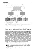
Second, link analysis can apply the concepts generated by visualization to
larger sets of customers. For instance, a churn reduction program might avoid
targeting customers who have high inertia or be sure to target customers with
high influence. This requires traversing the call graph to calculate the inertia or
influence for all customers. Such derived characteristics can play an important
role in marketing efforts.
Different marketing programs might suggest looking for other features in
the call graph. For instance, perhaps the ability to place a conference call
would be desirable, but who would be the best prospects? One idea would be
to look for groups of customers that all call each other. Stated as a graph prob-
lem, this group is a fully connected subgraph. In the telephone industry, these
subgraphs are called “communities of interest.” A community of interest may
represent a group of customers who would be interested in the ability to place
conference calls.
Lessons Learned
Link analysis is an application of the mathematical field of graph theory. As a
data mining technique, link analysis has several strengths:
■■ It capitalizes on relationships.
■■ It is useful for visualization.
■■ It creates derived characteristics that can be used for further mining.
Some data and data mining problems naturally involve links. As the two
case studies about telephone data show, link analysis is very useful for
telecommunications—a telephone call is a link between two people. Opportu-
nities for link analysis are most obvious in fields where the links are obvious
such as telephony, transportation, and the World Wide Web. Link analysis is
also appropriate in other areas where the connections do not have such a clear
manifestation, such as physician referral patterns, retail sales data, and foren-
sic analysis for crimes.
Links are a very natural way to visualize some types of data. Direct visual-

ization of the links can be a big aid to knowledge discovery. Even when auto-
mated patterns are found, visualization of the links helps to better understand
what is happening. Link analysis offers an alternative way of looking at data,
different from the formats of relational databases and OLAP tools. Links may
suggest important patterns in the data, but the significance of the patterns
requires a person for interpretation.
Link analysis can lead to new and useful data attributes. Examples include
calculating an authority score for a page on the World Wide Web and calculat-
ing the sphere of influence for a telephone user.
470643 c10.qxd 3/8/04 11:16 AM Page 347
Link Analysis 347
Although link analysis is very powerful when applicable, it is not appropri-
ate for all types of problems. It is not a prediction tool or classification tool like
a neural network that takes data in and produces an answer. Many types of
data are simply not appropriate for link analysis. Its strongest use is probably
in finding specific patterns, such as the types of outgoing calls, which can then
be applied to data. These patterns can be turned into new features of the data,
for use in conjunction with other directed data mining techniques.
470643 c10.qxd 3/8/04 11:16 AM Page 348
470643 c11.qxd 3/8/04 11:16 AM Page 349
11
Automatic Cluster Detection
CHAPTER
The data mining techniques described in this book are used to find meaning-
ful patterns in data. These patterns are not always immediately forthcoming.
Sometimes this is because there are no patterns to be found. Other times, the
problem is not the lack of patterns, but the excess. The data may contain so
much complex structure that even the best data mining techniques are unable
to coax out meaningful patterns. When mining such a database for the answer
to some specific question, competing explanations tend to cancel each other

out. As with radio reception, too many competing signals add up to noise.
Clustering provides a way to learn about the structure of complex data, to
break up the cacophony of competing signals into its components.
When human beings try to make sense of complex questions, our natural
tendency is to break the subject into smaller pieces, each of which can be
explained more simply. If someone were asked to describe the color of trees in
the forest, the answer would probably make distinctions between deciduous
trees and evergreens, and between winter, spring, summer, and fall. People
know enough about woodland flora to predict that, of all the hundreds of vari-
ables associated with the forest, season and foliage type, rather than say age
and height, are the best factors to use for forming clusters of trees that follow
similar coloration rules.
Once the proper clusters have been defined, it is often possible to find simple
patterns within each cluster. “In Winter, deciduous trees have no leaves so the
trees tend to be brown” or “The leaves of deciduous trees change color in the
349
470643 c11.qxd 3/8/04 11:16 AM Page 350
350 Chapter 11
autumn, typically to oranges, reds, and yellows.” In many cases, a very noisy
dataset is actually composed of a number of better-behaved clusters. The ques-
tion is: how can these be found? That is where techniques for automatic cluster
detection come in—to help see the forest without getting lost in the trees.
This chapter begins with two examples of the usefulness of clustering—one
drawn from astronomy, another from clothing design. It then introduces the
K-Means clustering algorithm which, like the nearest neighbor techniques dis-
cussed in Chapter 8, depends on a geometric interpretation of data. The geo-
metric ideas used in K-Means bring up the more general topic of measures of
similarity, association, and distance. These distance measures are quite sensi-
tive to variations in how data is represented, so the next topic addressed is
data preparation for clustering, with special attention being paid to scaling

and weighting. K-Means is not the only algorithm in common use for auto-
matic cluster detection. This chapter contains brief discussions of several
others: Gaussian mixture models, agglomerative clustering, and divisive clus-
tering. (Another clustering technique, self-organizing maps, is covered in
Chapter 7 because self-organizing maps are a form of neural network.) The
chapter concludes with a case study in which automatic cluster detection is
used to evaluate editorial zones for a major daily newspaper.
Searching for Islands of Simplicity
In Chapter 1, where data mining techniques are classified as directed or undi-
rected, automatic cluster detection is described as a tool for undirected knowl-
edge discovery. In the technical sense, that is true because the automatic
cluster detection algorithms themselves are simply finding structure that
exists in the data without regard to any particular target variable. Most data
mining tasks start out with a preclassified training set, which is used to
develop a model capable of scoring or classifying previously unseen records.
In clustering, there is no preclassified data and no distinction between inde-
pendent and dependent variables. Instead, clustering algorithms search for
groups of records—the clusters—composed of records similar to each other.
The algorithms discover these similarities. It is up to the people running the
analysis to determine whether similar records represent something of interest
to the business—or something inexplicable and perhaps unimportant.
In a broader sense, however, clustering can be a directed activity because
clusters are sought for some business purpose. In marketing, clusters formed
for a business purpose are usually called “segments,” and customer segmen-
tation is a popular application of clustering.
Automatic cluster detection is a data mining technique that is rarely used in
isolation because finding clusters is not often an end in itself. Once clusters
have been detected, other methods must be applied in order to figure out what
470643 c11.qxd 3/8/04 11:16 AM Page 351
Automatic Cluster Detection 351

the clusters mean. When clustering is successful, the results can be dramatic:
One famous early application of cluster detection led to our current under-
standing of stellar evolution.
Star Light, Star Bright
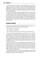
Early in the twentieth century, astronomers trying to understand the relation-
ship between the luminosity (brightness) of stars and their temperatures,
made scatter plots like the one in Figure 11.1. The vertical scale measures lumi-
nosity in multiples of the brightness of our own sun. The horizontal scale
measures surface temperature in degrees Kelvin (degrees centigrade above
absolute 0, the theoretical coldest possible temperature).
10
6
10
4
10
2
1
10
-2
10
-4
Red Giants
40,000 20,000 10,000 5,000 2,500
Main Sequence
White Dwarfs
Luminosity (Sun = 1)
Temperature (Degrees Kelvin)
Figure 11.1 The Hertzsprung-Russell diagram clusters stars by temperature and luminosity.
470643 c11.qxd 3/8/04 11:16 AM Page 352
352 Chapter 11

Two different astronomers, Enjar Hertzsprung in Denmark and Norris
Russell in the United States, thought of doing this at about the same time. They
both observed that in the resulting scatter plot, the stars fall into three clusters.
This observation led to further work and the understanding that these three
clusters represent stars in very different phases of the stellar life cycle. The rela-
tionship between luminosity and temperature is consistent within each cluster,
but the relationship is different between the clusters because fundamentally
different processes are generating the heat and light. The 80 percent of stars that
fall on the main sequence are generating energy by converting hydrogen to
helium through nuclear fusion. This is how all stars spend most of their active
life. After some number of billions of years, the hydrogen is used up. Depend-
ing on its mass, the star then begins fusing helium or the fusion stops. In the lat-
ter case, the core of the star collapses, generating a great deal of heat in the
process. At the same time, the outer layer of gasses expands away from the core,
and a red giant is formed. Eventually, the outer layer of gasses is stripped away,
and the remaining core begins to cool. The star is now a white dwarf.
A recent search on Google using the phrase “Hertzsprung-Russell Diagram”
returned thousands of pages of links to current astronomical research based on
cluster detection of this kind. Even today, clusters based on the HR diagram
are being used to hunt for brown dwarfs (starlike objects that lack sufficient
mass to initiate nuclear fusion) and to understand pre–main sequence stellar
evolution.
Fitting the Troops
The Hertzsprung-Russell diagram is a good introductory example of cluster-
ing because with only two variables, it is easy to spot the clusters visually
(and, incidentally, it is a good example of the importance of good data visual-
izations). Even in three dimensions, picking out clusters by eye from a scatter
plot cube is not too difficult. If all problems had so few dimensions, there
would be no need for automatic cluster detection algorithms. As the number
of dimensions (independent variables) increases, it becomes increasing diffi-

cult to visualize clusters. Our intuition about how close things are to each
other also quickly breaks down with more dimensions.
Saying that a problem has many dimensions is an invitation to analyze it
geometrically. A dimension is each of the things that must be measured inde-
pendently in order to describe something. In other words, if there are N vari-
ables, imagine a space in which the value of each variable represents a distance
along the corresponding axis in an N-dimensional space. A single record con-
taining a value for each of the N variables can be thought of as the vector that
defines a particular point in that space. When there are two dimensions, this is
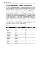
easily plotted. The HR diagram was one such example. Figure 11.2 is another
example that plots the height and weight of a group of teenagers as points on
a graph. Notice the clustering of boys and girls.
TEAMFLY

Team-Fly
®

470643 c11.qxd 3/8/04 11:17 AM Page 353
Automatic Cluster Detection 353
The chart in Figure 11.2 begins to give a rough idea of people’s shapes. But
if the goal is to fit them for clothes, a few more measurements are needed!
In the 1990s, the U.S. army commissioned a study on how to redesign the
uniforms of female soldiers. The army’s goal was to reduce the number of dif-
Height (Inches)
ferent uniform sizes that have to be kept in inventory, while still providing
each soldier with well-fitting uniforms.
As anyone who has ever shopped for women’s clothing is aware, there is
already a surfeit of classification systems (even sizes, odd sizes, plus sizes,
junior, petite, and so on) for categorizing garments by size. None of these
systems was designed with the needs of the U.S. military in mind. Susan
Ashdown and Beatrix Paal, researchers at Cornell University, went back to the
basics; they designed a new set of sizes based on the actual shapes of women
in the army.
1
80
75
70
65

60
100 125 150 175 200
Weight (Pounds)
Figure 11.2 Heights and weights of a group of teenagers.
1
Ashdown, Susan P. 1998. “An Investigation of the Structure of Sizing Systems: A Comparison of
Three Multidimensional Optimized Sizing Systems Generated from Anthropometric Data,”
International Journal of Clothing Science and Technology. Vol. 10, #5, pp 324-341.
470643 c11.qxd 3/8/04 11:17 AM Page 354
354 Chapter 11
Unlike the traditional clothing size systems, the one Ashdown and Paal came
up with is not an ordered set of graduated sizes where all dimensions increase
together. Instead, they came up with sizes that fit particular body types. Each
body type corresponds to a cluster of records in a database of body measure-
ments. One cluster might consist of short-legged, small-waisted, large-busted
women with long torsos, average arms, broad shoulders, and skinny necks
while other clusters capture other constellations of measurements.
The database contained more than 100 measurements for each of nearly
3,000 women. The clustering technique employed was the K-means algorithm,
described in the next section. In the end, only a handful of the more than 100
measurements were needed to characterize the clusters. Finding this smaller
number of variables was another benefit of the clustering process.
K-Means Clustering
The K-means algorithm is one of the most commonly used clustering algo-
rithms. The “K” in its name refers to the fact that the algorithm looks for a fixed
number of clusters which are defined in terms of proximity of data points to
each other. The version described here was first published by J. B. MacQueen in
1967. For ease of explaining, the technique is illustrated using two-dimensional
diagrams. Bear in mind that in practice the algorithm is usually handling many
more than two independent variables. This means that instead of points corre-

sponding to two-element vectors (x
1
,x
2
), the points correspond to n-element
vectors (x
1
,x
2
, . . . , x
n
). The procedure itself is unchanged.
Three Steps of the K-Means Algorithm
In the first step, the algorithm randomly selects K data points to be the seeds.
MacQueen’s algorithm simply takes the first K records. In cases where the
records have some meaningful order, it may be desirable to choose widely
spaced records, or a random selection of records. Each of the seeds is an
embryonic cluster with only one element. This example sets the number of
clusters to 3.
The second step assigns each record to the closest seed. One way to do this
is by finding the boundaries between the clusters, as shown geometrically
in Figure 11.3. The boundaries between two clusters are the points that are
equally close to each cluster. Recalling a lesson from high-school geometry
makes this less difficult than it sounds: given any two points, A and B, all
points that are equidistant from A and B fall along a line (called the perpen-
dicular bisector) that is perpendicular to the one connecting A and B and
halfway between them. In Figure 11.3, dashed lines connect the initial seeds;
the resulting cluster boundaries shown with solid lines are at right angles to
470643 c11.qxd 3/8/04 11:17 AM Page 355
Automatic Cluster Detection 355

the dashed lines. Using these lines as guides, it is obvious which records are
closest to which seeds. In three dimensions, these boundaries would be planes
and in N dimensions they would be hyperplanes of dimension N – 1. Fortu-
nately, computer algorithms easily handle these situations. Finding the actual
boundaries between clusters is useful for showing the process geometrically.
In practice, though, the algorithm usually measures the distance of each record
to each seed and chooses the minimum distance for this step.
For example, consider the record with the box drawn around it. On the basis
of the initial seeds, this record is assigned to the cluster controlled by seed
number 2 because it is closer to that seed than to either of the other two.
At this point, every point has been assigned to exactly one of the three clus-
ters centered around the original seeds. The third step is to calculate the cen-
troids of the clusters; these now do a better job of characterizing the clusters
than the initial seeds Finding the centroids is simply a matter of taking the
average value of each dimension for all the records in the cluster.
In Figure 11.4, the new centroids are marked with a cross. The arrows show
the motion from the position of the original seeds to the new centroids of the
clusters formed from those seeds.
X
2
X
1
Seed 3
Seed 1
Seed 2
Figure 11.3 The initial seeds determine the initial cluster boundaries.
470643 c11.qxd 3/8/04 11:17 AM Page 356
356 Chapter 11
X
2

X
1
Figure 11.4 The centroids are calculated from the points that are assigned to each cluster.
The centroids become the seeds for the next iteration of the algorithm. Step 2
is repeated, and each point is once again assigned to the cluster with the closest
centroid. Figure 11.5 shows the new cluster boundaries—formed, as before, by
drawing lines equidistant between each pair of centroids. Notice that the point
with the box around it, which was originally assigned to cluster number 2, has
now been assigned to cluster number 1. The process of assigning points to clus-
ter and then recalculating centroids continues until the cluster boundaries
stop changing. In practice, the K-means algorithm usually finds a set of stable
clusters after a few dozen iterations.
What K Means
Clusters describe underlying structure in data. However, there is no one right
description of that structure. For instance, someone not from New York City
may think that the whole city is “downtown.” Someone from Brooklyn or
Queens might apply this nomenclature to Manhattan. Within Manhattan, it
might only be neighborhoods south of 23
rd
Street. And even there, “down-
town” might still be reserved only for the taller buildings at the southern tip of
the island. There is a similar problem with clustering; structures in data exist
at many different levels.
470643 c11.qxd 3/8/04 11:17 AM Page 357
Automatic Cluster Detection 357
X
2
X
1
Figure 11.5 At each iteration, all cluster assignments are reevaluated.

Descriptions of K-means and related algorithms gloss over the selection of
K. But since, in many cases, there is no a priori reason to select a particular
value, there is really an outermost loop to these algorithms that occurs during
analysis rather than in the computer program. This outer loop consists of per-
forming automatic cluster detection using one value of K, evaluating the
results, then trying again with another value of K or perhaps modifying the
data. After each trial, the strength of the resulting clusters can be evaluated by
comparing the average distance between records in a cluster with the average
distance between clusters, and by other procedures described later in this
chapter. These tests can be automated, but the clusters must also be evaluated
on a more subjective basis to determine their usefulness for a given applica-
tion. As shown in Figure 11.6, different values of K may lead to very different
clusterings that are equally valid. The figure shows clusterings of a deck of
playing cards for K = 2 and K = 4. Is one better than the other? It depends on
the use to which the clusters will be put.
Figure 11.6 These examples of clusters of size 2 and 4 in a deck of playing cards illustrate
that there is no one correct clustering.
Often the first time K-means clustering is run on a given set of data, most
of the data points fall in one giant central cluster and there are a number of
smaller clusters outside it. This is often because most records describe “nor-
mal” variations in the data, but there are enough outliers to confuse the clus-
tering algorithm. This type of clustering may be valuable for applications such
as identifying fraud or manufacturing defects. In other applications, it may be
desirable to filter outliers from the data; more often, the solution is to massage
the data values. Later in this chapter there is a section on data preparation for
clustering which describes how to work with variables to make it easier to find
meaningful clusters.
Similarity and Distance
Once records in a database have been mapped to points in space, automatic
cluster detection is really quite simple—a little geometry, some vector means,

et voilà! The problem, of course, is that the databases encountered in market-
ing, sales, and customer support are not about points in space. They are about
purchases, phone calls, airplane trips, car registrations, and a thousand other
things that have no obvious connection to the dots in a cluster diagram.
Clustering records of this sort requires some notion of natural association;
that is, records in a given cluster are more similar to each other than to records
in another cluster. Since it is difficult to convey intuitive notions to a computer,
358 Chapter 11
470643 c11.qxd 3/8/04 11:17 AM Page 358
470643 c11.qxd 3/8/04 11:17 AM Page 359
Automatic Cluster Detection 359
this vague concept of association must be translated into some sort of numeric
measure of the degree of similarity. The most common method, but by no
means the only one, is to translate all fields into numeric values so that the
records may be treated as points in space. Then, if two points are close in
the geometric sense, they represent similar records in the database. There are
two main problems with this approach:
■■ Many variable types, including all categorical variables and many
numeric variables such as rankings, do not have the right behavior to
properly be treated as components of a position vector.
■■ In geometry, the contributions of each dimension are of equal impor-
tance, but in databases, a small change in one field may be much more
important than a large change in another field.
The following section introduces several alternative measures of similarity.
Similarity Measures and Variable Type
Geometric distance works well as a similarity measure for well-behaved
numeric variables. A well-behaved numeric variable is one whose value indi-
cates its placement along the axis that corresponds to it in our geometric
model. Not all variables fall into this category. For this purpose, variables fall
into four classes, listed here in increasing order of suitability for the geometric

model.
■■ Categorical variables
■■ Ranks
■■ Intervals
■■ True measures
Categorical variables only describe which of several unordered categories a
thing belongs to. For instance, it is possible to label one ice cream pistachio and
another butter pecan, but it is not possible to say that one is greater than the
other or judge which one is closer to black cherry. In mathematical terms, it is
possible to tell that X ≠ Y, but not whether X > Y or X < Y.
Ranks put things in order, but don’t say how much bigger one thing is than
another. The valedictorian has better grades than the salutatorian, but we
don’t know by how much. If X, Y, and Z are ranked A, B, and C, we know that
X > Y > Z, but we cannot define X-Y or Y-Z .
Intervals measure the distance between two observations. If it is 56° in San
Francisco and 78° in San Jose, then it is 22 degrees warmer at one end of the
bay than the other.
470643 c11.qxd 3/8/04 11:17 AM Page 360
360 Chapter 11
True measures are interval variables that measure from a meaningful zero
point. This trait is important because it means that the ratio of two values of
the variable is meaningful. The Fahrenheit temperature scale used in the
United States and the Celsius scale used in most of the rest of the world do not
have this property. In neither system does it make sense to say that a 30° day is
twice as warm as a 15° day. Similarly, a size 12 dress is not twice as large as a
size 6, and gypsum is not twice as hard as talc though they are 2 and 1 on the
hardness scale. It does make perfect sense, however, to say that a 50-year-old
is twice as old as a 25-year-old or that a 10-pound bag of sugar is twice as
heavy as a 5-pound one. Age, weight, length, customer tenure, and volume are
examples of true measures.

Geometric distance metrics are well-defined for interval variables and true
measures. In order to use categorical variables and rankings, it is necessary to
transform them into interval variables. Unfortunately, these transformations
may add spurious information. If ice cream flavors are assigned arbitrary
numbers 1 through 28, it will appear that flavors 5 and 6 are closely related
while flavors 1 and 28 are far apart.
These and other data transformation and preparation issues are discussed
extensively in Chapter 17.
Formal Measures of Similarity
There are dozens if not hundreds of published techniques for measuring the
similarity of two records. Some have been developed for specialized applica-
tions such as comparing passages of text. Others are designed especially for
use with certain types of data such as binary variables or categorical variables.
Of the three presented here, the first two are suitable for use with interval vari-
ables and true measures, while the third is suitable for categorical variables.
Geometric Distance between Two Points
When the fields in a record are numeric, the record represents a point in
n-dimensional space. The distance between the points represented by two
records is used as the measure of similarity between them. If two points are
close in distance, the corresponding records are similar.
There are many ways to measure the distance between two points, as
discussed in the sidebar “Distance Metrics”. The most common one is the
Euclidian distance familiar from high-school geometry. To find the Euclidian
distance between X and Y, first find the differences between the corresponding
elements of X and Y (the distance along each axis) and square them. The dis-
tance is the square root of the sum of the squared differences.
470643 c11.qxd 3/8/04 11:17 AM Page 361
Automatic Cluster Detection 361
Any function that takes two points and produces a single number describing a
◆ Distance(X,Y) = 0 if and only if X = Y

◆ Distance(X,Y) ≥ 0 for all X and all Y
◆ Distance(X,Y) = Distance(Y,X)
◆ Distance(X,Y) ≤ Distance(X,Z) + Distance(Z,Y)
identity and commutativity by mathematicians)—that the measure is 0 or
positive and is well-defined for any two points. If two records have a distance
DISTANCE METRICS
relationship between them is a candidate measure of similarity, but to be a true
distance metric, it must meet the following criteria:
These are the formal definition of a distance metric in geometry.
A true distance is a good metric for clustering, but some of these conditions
can be relaxed. The most important conditions are the second and third (called
of 0, that is okay, as long as they are very, very similar, since they will always
fall into the same cluster.
The last condition, the Triangle Inequality, is perhaps the most interesting
mathematically. In terms of clustering, it basically means that adding a new
cluster center will not make two distant points suddenly seem close together.
Fortunately, most metrics we could devise satisfy this condition.
Angle between Two Vectors
Sometimes it makes more sense to consider two records closely associated
because of similarities in the way the fields within each record are related. Min-
nows should cluster with sardines, cod, and tuna, while kittens cluster with
cougars, lions, and tigers, even though in a database of body-part lengths, the
sardine is closer to a kitten than it is to a catfish.
The solution is to use a different geometric interpretation of the same data.
Instead of thinking of X and Y as points in space and measuring the distance
between them, think of them as vectors and measure the angle between them.
In this context, a vector is the line segment connecting the origin of a coordi-
nate system to the point described by the vector values. A vector has both mag-
nitude (the distance from the origin to the point) and direction. For this
similarity measure, it is the direction that matters.

Take the values for length of whiskers, length of tail, overall body length,
length of teeth, and length of claws for a lion and a house cat and plot them as
single points, they will be very far apart. But if the ratios of lengths of these
body parts to one another are similar in the two species, than the vectors will
be nearly colinear.
470643 c11.qxd 3/8/04 11:17 AM Page 362
362 Chapter 11
The angle between vectors provides a measure of association that is not
influenced by differences in magnitude between the two things being com-
pared (see Figure 11.7). Actually, the sine of the angle is a better measure since
it will range from 0 when the vectors are closest (most nearly parallel) to 1
when they are perpendicular. Using the sine ensures that an angle of 0 degrees
is treated the same as an angle of 180 degrees, which is as it should be since for
this measure, any two vectors that differ only by a constant factor are consid-
ered similar, even if the constant factor is negative. Note that the cosine of the
angle measures correlation; it is 1 when the vectors are parallel (perfectly
correlated) and 0 when they are orthogonal.
Big Fish
Little Fish
Big Cat
Little Cat
Figure 11.7 The angle between vectors as a measure of similarity.
TEAMFLY

Team-Fly
®

470643 c11.qxd 3/8/04 11:17 AM Page 363
Automatic Cluster Detection 363
Manhattan Distance
Another common distance metric gets its name from the rectangular grid pat-
tern of streets in midtown Manhattan. It is simply the sum of the distances
traveled along each axis. This measure is sometimes preferred to the Euclidean
distance because given that the distances along each axis are not squared, it
is less likely that a large difference in one dimension will dominate the total
distance.
Number of Features in Common
When the preponderance of fields in the records are categorical variables, geo-

metric measures are not the best choice. A better measure is based on the
degree of overlap between records. As with the geometric measures, there are
many variations on this idea. In all variations, the two records are compared
field by field to determine the number of fields that match and the number of
fields that don’t match. The simplest measure is the ratio of matches to the
total number of fields.
In its simplest form, this measure counts two null or empty fields as match-
ing. This has the perhaps perverse result that everything with missing data
ends up in the same cluster. A simple improvement is to not include matches of
this sort in the match count. Another improvement is to weight the matches by
the prevalence of each class in the general population. After all, a match on
“Chevy Nomad” ought to count for more than a match on “Ford F-150 Pickup.”
Data Preparation for Clustering
The notions of scaling and weighting each play important roles in clustering.
Although similar, and often confused with each other, the two notions are not
the same. Scaling adjusts the values of variables to take into account the fact
that different variables are measured in different units or over different ranges.
For instance, household income is measured in tens of thousands of dollars
and number of children in single digits. Weighting provides a relative adjust-
ment for a variable, because some variables are more important than others.
Scaling for Consistency
In geometry, all dimensions are equally important. Two points that differ by 2
in dimensions X and Y and by 1 in dimension Z are the same distance apart as
two other points that differ by 1 in dimension X and by 2 in dimensions Y and
Z. It doesn’t matter what units X, Y, and Z are measured in, so long as they are
the same.
470643 c11.qxd 3/8/04 11:17 AM Page 364
364 Chapter 11
But what if X is measured in yards, Y is measured in centimeters, and Z is
measured in nautical miles? A difference of 1 in Z is now equivalent to a dif-

ference of 185,200 in Y or 2,025 in X. Clearly, they must all be converted to a
common scale before distances will make any sense.
Unfortunately, in commercial data mining there is usually no common scale
available because the different units being used are measuring quite different
things. If variables include plot size, number of children, car ownership, and
family income, they cannot all be converted to a common unit. On the other
hand, it is misleading that a difference of 20 acres is indistinguishable from
a change of $20. One solution is to map all the variables to a common
range (often 0 to 1 or –1 to 1). That way, at least the ratios of change become
comparable—doubling the plot size has the same effect as doubling income.
Scaling solves this problem, in this case by remapping to a common range.
TIP It is very important to scale different variables so their values fall roughly
into the same range, by normalizing, indexing, or standardizing the values.
Here are three common ways of scaling variables to bring them all into com-
parable ranges:
■■ Divide each variable by the range (the difference between the lowest
and highest value it takes on) after subtracting the lowest value. This
maps all values to the range 0 to 1, which is useful for some data
mining algorithms.
■■ Divide each variable by the mean of all the values it takes on. This is
often called “indexing a variable.”
■■ Subtract the mean value from each variable and then divide it by the
standard deviation. This is often called standardization or “converting to
z-scores.” A z-score tells you how many standard deviations away from
the mean a value is.
Normalizing a single variable simply changes its range. A closely related
concept is vector normalization which scales all variables at once. This too has a
geometric interpretation. Consider the collection of values in a single record or
observation as a vector. Normalizing them scales each value so as to make the
length of the vector equal one. Transforming all the vectors to unit length

emphasizes the differences internal to each record rather than the differences
between records. As an example, consider two records with fields for debt and
equity. The first record contains debt of $200,000 and equity of $100,000; the
second, debt of $10,000 and equity of $5,000. After normalization, the two
records look the same since both have the same ratio of debt to equity.
470643 c11.qxd 3/8/04 11:17 AM Page 365
Automatic Cluster Detection 365
Use Weights to Encode Outside Information
Scaling takes care of the problem that changes in one variable appear more
significant than changes in another simply because of differences in the
magnitudes of the values in the variable. What if we think that two families
with the same income have more in common than two families on the same
size plot, and we want that to be taken into consideration during clustering?
That is where weighting comes in. The purpose of weighting is to encode the
information that one variable is more (or less) important than others.
A good place to starts is by standardizing all variables so each has a mean of
zero and a variance (and standard deviation) of one. That way, all fields con-
tribute equally when the distance between two records is computed.
We suggest going farther. The whole point of automatic cluster detection is
to find clusters that make sense to you. If, for your purposes, whether people
have children is much more important than the number of credit cards they
carry, there is no reason not to bias the outcome of the clustering by multiply-
ing the number of children field by a higher weight than the number of credit
cards field. After scaling to get rid of bias that is due to the units, use weights
to introduce bias based on knowledge of the business context.
Some clustering tools allow the user to attach weights to different dimen-
sions, simplifying the process. Even for tools that don’t have such functionality,
it is possible to have weights by adjusting the scaled values. That is, first scale
the values to a common range to eliminate range effects. Then multiply the
resulting values by a weight to introduce bias based on the business context.

Of course, if you want to evaluate the effects of different weighting strate-
gies, you will have to add another outer loop to the clustering process.
Other Approaches to Cluster Detection
The basic K-means algorithm has many variations. Many commercial software
tools that include automatic cluster detection incorporate some of these varia-
tions. Among the differences are alternate methods of choosing the initial
seeds and the use of probability density rather than distance to associate
records with clusters. This last variation merits additional discussion. In addi-
tion, there are several different approaches to clustering, including agglomer-
ative clustering, divisive clustering, and self organizing maps.
Gaussian Mixture Models
The K-means method as described has some drawbacks:
■■ It does not do well with overlapping clusters.
■■ The clusters are easily pulled off-center by outliers.
■■ Each record is either inside or outside of a given cluster.
470643 c11.qxd 3/8/04 11:17 AM Page 366
366 Chapter 11
Gaussian mixture models are a probabilistic variant of K-means. The name
comes from the Gaussian distribution, a probability distribution often
assumed for high-dimensional problems. The Gaussian distribution general-
izes the normal distribution to more than one variable. As before, the algo-
rithm starts by choosing K seeds. This time, however, the seeds are considered
to be the means of Gaussian distributions. The algorithm proceeds by iterating
over two steps called the estimation step and the maximization step.
The estimation step calculates the responsibility that each Gaussian has for
each data point (see Figure 11.8). Each Gaussian has strong responsibility
for points that are close to its mean and weak responsibility for points that are
distant. The responsibilities are be used as weights in the next step.
In the maximization step, a new centroid is calculated for each cluster
taking into account the newly calculated responsibilities. The centroid for a

given Gaussian is calculated by averaging all the points weighted by the respon-
sibilities for that Gaussian, as illustrated in Figure 11.9.
X
2
X
1
G1
G2
G3
Figure 11.8 In the estimation step, each Gaussian is assigned some responsibility for each
point. Thicker lines indicate greater responsibility.
470643 c11.qxd 3/8/04 11:17 AM Page 367
Automatic Cluster Detection 367
These steps are repeated until the Gaussians no longer move. The Gaussians
themselves can change in shape as well as move. However, each Gaussian is
constrained, so if it shows a very high responsibility for points close to its mean,
then there is a sharp drop off in responsibilities. If the Gaussian covers a larger
range of values, then it has smaller responsibilities for nearby points. Since the
distribution must always integrate to one, Gaussians always gets weaker as
they get bigger.
The reason this is called a “mixture model” is that the probability at each
data point is the sum of a mixture of several distributions. At the end of the
process, each point is tied to the various clusters with higher or lower proba-
bility. This is sometimes called soft clustering, because points are not uniquely
identified with a single cluster.
One consequence of this method is that some points may have high proba-
bilities of being in more than one cluster. Other points may have only very low
probabilities of being in any cluster. Each point can be assigned to the cluster
where its probability is highest, turning this soft clustering into hard clustering.
X

2
X
1
Figure 11.9 Each Gaussian mean is moved to the centroid of all the data points weighted
by its responsibilities for each point. Thicker arrows indicate higher weights.
470643 c11.qxd 3/8/04 11:17 AM Page 368
368 Chapter 11
Agglomerative Clustering
The K-means approach to clustering starts out with a fixed number of clusters
and allocates all records into exactly that number of clusters. Another class of
methods works by agglomeration. These methods start out with each data point
forming its own cluster and gradually merge them into larger and larger clusters
until all points have been gathered together into one big cluster. Toward the
beginning of the process, the clusters are very small and very pure—the members
of each cluster are few and closely related. Towards the end of the process, the
clusters are large and not as well defined. The entire history is preserved making
it possible to choose the level of clustering that works best for a given application.
An Agglomerative Clustering Algorithm
The first step is to create a similarity matrix. The similarity matrix is a table of
all the pair-wise distances or degrees of similarity between clusters. Initially,
the similarity matrix contains the pair-wise distance between individual pairs
of records. As discussed earlier, there are many measures of similarity between
records, including the Euclidean distance, the angle between vectors, and the
ratio of matching to nonmatching categorical fields. The issues raised by the
choice of distance measures are exactly the same as those previously discussed
in relation to the K-means approach.
It might seem that with N initial clusters for N data points, N
2
measurement
calculations are required to create the distance table. If the similarity measure

is a true distance metric, only half that is needed because all true distance met-
rics follow the rule that Distance(X,Y) = Distance(Y,X). In the vocabulary of
mathematics, the similarity matrix is lower triangular. The next step is to find
the smallest value in the similarity matrix. This identifies the two clusters that
are most similar to one another. Merge these two clusters into a new one and
update the similarity matrix by replacing the two rows that described the par-
ent cluster with a new row that describes the distance between the merged
cluster and the remaining clusters. There are now N – 1 clusters and N – 1 rows
in the similarity matrix.
Repeat the merge step N – 1 times, so all records belong to the same large
cluster. Each iteration remembers which clusters were merged and the dis-
tance between them. This information is used to decide which level of cluster-
ing to make use of.
Distance between Clusters
A bit more needs to be said about how to measure distance between clusters.
On the first trip through the merge step, the clusters consist of single records
so the distance between clusters is the same as the distance between records, a
subject that has already been covered in perhaps too much detail. Second and
470643 c11.qxd 3/8/04 11:17 AM Page 369
Automatic Cluster Detection 369
subsequent trips through the loop need to update the similarity matrix with
the distances from the new, multirecord cluster to all the others. How do we
measure this distance?
As usual, there is a choice of approaches. Three common ones are:
■■ Single linkage
■■ Complete linkage
■■ Centroid distance
In the single linkage method, the distance between two clusters is given by the
distance between the closest members. This method produces clusters with the
property that every member of a cluster is more closely related to at least one

member of its cluster than to any point outside it.
Another approach is the complete linkage method, where the distance between
two clusters is given by the distance between their most distant members. This
method produces clusters with the property that all members lie within some
known maximum distance of one another.
Third method is the centroid distance, where the distance between two clusters
is measured between the centroids of each. The centroid of a cluster is its average
element. Figure 11.10 gives a pictorial representation of these three methods.
X
2
X
1
Closest clusters by
centroid method
C1
C2
C3
Closest clusters by
complete linkage method
Closest clusters by
single linkage method
Figure 11.10 Three methods of measuring the distance between clusters.
470643 c11.qxd 3/8/04 11:17 AM Page 370
370 Chapter 11
Clusters and Trees
The agglomeration algorithm creates hierarchical clusters. At each level in the
hierarchy, clusters are formed from the union of two clusters at the next level
down. A good way of visualizing these clusters is as a tree. Of course, such a
tree may look like the decision trees discussed in Chapter 6, but there are some
important differences. The most important is that the nodes of the cluster tree

do not embed rules describing why the clustering takes place; the nodes sim-
ply state the fact that the two children have the minimum distance of all pos-
sible clusters pairs. Another difference is that a decision tree is created to
maximize the leaf purity of a given target variable. There is no target for the
cluster tree, other than self-similarity within each cluster. Later in this chapter
we’ll discuss divisive clustering methods. These are similar to the agglomera-
tive methods, except that agglomerative methods are build by starting from
the leaving and working towards the root whereas divisive methods start at
the root and work down to the leaves.
Clustering People by Age: An Example of
Agglomerative Clustering
This illustration of agglomerative clustering uses an example in one dimen-
sion with the single linkage measure for distance between clusters. These
choices make it possible to follow the algorithm through all its iterations with-
out having to worry about calculating distances using squares and square
roots.
The data consists of the ages of people at a family gathering. The goal is to
cluster the participants using their age, and the metric for the distance between
two people is simply the difference in their ages. The metric for the distance
between two clusters of people is the difference in age between the oldest
member of the younger cluster and the youngest member of the older cluster.
(The one dimensional version of the single linkage measure.)
Because the distances are so easy to calculate, the example dispenses with
the similarity matrix. The procedure is to sort the participants by age, then
begin clustering by first merging clusters that are 1 year apart, then 2 years,
and so on until there is only one big cluster.
Figure 11.11 shows the clusters after six iterations, with three clusters
remaining. This is the level of clustering that seems the most useful. The
algorithm appears to have clustered the population into three generations:
children, parents, and grandparents.