Báo cáo hóa học: "Research Article Decentralized Turbo Báo cáo hóa học: "Bayesian Compressed Sensing with Application to UWB Systems" potx

Hindawi Publishing Corporation
EURASIP Journal on Advances in Signal Processing
Volume 2011, Article ID 817947, 17 pages
doi:10.1155/2011/817947
Research Article
Decentralized Turbo Bayesian Compressed Sensing with
Application to UWB Systems
Depeng Yang, Husheng Li, and Gregory D. Peterson
Department of Electrical Eng ineering and Computer Science, The University of Tennessee, Knoxville, TN 37996, USA
Correspondence should be addressed to Depeng Yang,
Received 19 July 2010; Revised 1 February 2011; Accepted 28 February 2011
Academic Editor: Dirk T. M. Slock
Copyright © 2011 Depeng Yang et al. This is an open access article distributed under the Creative Commons Attribution License,
which permits unrestricted use, distribution, and reproduction in any medium, provided the original work i s properly cited.
In many situations, there exist plenty of spatial and temporal redundancies in original signals. Based on this observation, a novel
Turbo Bayesian Compressed Sensing (TBCS) algorithm is proposed to provide an efficient approach to transfer and incorporate
this redundant information for joint sparse signal reconstruction. As a case study, the TBCS algorithm is applied in Ultra-
Wideband (UWB) systems. A space-time TBCS structure is developed for exploiting and incorporating the spatial and temporal
aprioriinformation for space-time signal reconstruction. Simulation results demonstrate that the proposed TBCS algorithm
achieves much better performance with only a few measurements in the presence of noise, compared with the traditional Bayesian
Compressed Sensing (BCS) and multitask BCS algorithms.
1. Introduction
Compressed sensing (CS) theory [1, 2] is blooming in recent
years. In the CS theory, the original signal is not directly
acquired but reconstructed based on the measurements
obtained f rom projecting the signal using a random sensing
matrix. It is well known that most natural signals are sparse,
that is, in a certain transform domain, most elements are
zeros or have very small amplitudes. Taking advantage of
such sparsity, various CS signal reconstruction algorithms
are developed to recover the original signal from a few

observations and measurements [3–5].
In many situations, there are multiple copies of signals
that are correlated in space and time, thus providing
spatial and temporal redundancies. Take the CS-based Ultra-
Wideband (UWB) system as an example (A UWB system
utilizes a short-range, high-bandwidth pulse without carrier
frequency for communication, positioning, and radar imag-
ing. One challenge is the acquisition of the high-resolution
ultrashort duration pulses. The emergence of CS theory
provides an approach to acquiring UWB pulses, possibly
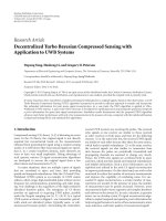
under the Nyquist sampling rate [6, 7].) [8, 9]. In a typical
UWB system as shown in Figure 1, one transmitter period-
ically sends out ultrashort pulses (typically nano- or sub-
nanosecond Gaussian pulses). Surrounding the transmitter,
several UWB receivers are receiving the pulses. The received
echo sig nals at one receiver are similar to those received
at other receivers in both space and time for the following
reasons: (1) at the same time slot, the received UWB signals
are similar to each other because they share the same source,
which l eads to spatial redundancy; (2) at the same receiver,
the received signals are also similar in consecutive time
slots because the pulses are periodically transmitted and
propagating channels are assumed to change very slowly.
Hence, the UWB echo signals are correlated both in space
and time, which provides spatial and temporal redundancies
and helpful information. Such aprioriinformation can be
exploited and utilized in the joint CS signal reconstruction
to improve performance. On the other hand, our work is also
motivated to reduce the number of necessary measurements
and improve the capability of combating noise. For suc-

cessful CS signal reconstruction, a certain number of mea-
surements are needed. In the presence of noise, the number
of measurement may be greatly increased. However, more
measurements lead to more expensive and complex hardware
and software in the system [6]. In such a situation, a question
arises: can we develop a joint CS signal reconstruction algo-
rithm to exploit temporal and spatial aprioriinformation for
improving performance in terms of less measurements, more
noise tolerance, and better quality of reconstructed signal?
2 EURASIP Journal on Advances in Signal Processing
UWB
transmitter
UWB
receiver
UWB
receiver
UWB
receiver
UWB
receiver
Figure 1: A typical UWB system with one transmitter and several
receivers.
Related research about joint CS signal reconstruction
has been developed in the literature recently. Distributed
compressed sensing (DCS) [10, 11] studies joint sparsity
and joint signal reconstruction. Simultaneous Orthogonal
Matching Pursuit (SOMP) [12, 13] for simultaneous signal
reconstruction is developed by extending the traditional
Orthogonal Matching Pursuit (OMP) algorithm. Serial OMP
[14] studies time sequence signal reconstruction. The joint

sparse recovery algorithm [15] is developed in association
with the basis pursuit (BP) algorithm. These algorithms
focus on either temporal or spatial joint signal reconstruc-
tion. T hey are developed by extending convex optimization
and linear programming algorithms but ignore the impact of
possible noise in the measurements.
Other work on sparse signal reconstruct ion is based on
a statistical Bayesian framework. In [16, 17], the authors
developed a sparse signal reconstruction algorithm based
on the belief propagation framework for the signal recon-
struction. The information is exchanged among different
elements in the signal vector in a way similar to the decoding
of low-density parity check (LDPC) codes. In [18], the
LDPC coding/decoding algorithm has been extended for
real number CS signal reconstruction. Other Bayesian CS
algorithms also have been developed in [3, 4, 19, 20]. In [3], a
pursuit method in the Bernoulli-Gaussian model is proposed
to search for the nonzero s ignal elements. A Bayesian
approach for Sparse Component Analysis for the noisy case is
presented in [4]. In [19], a Gaussian mixture is adopted as the
prior distribution in the Bayesian model, which has similar
performance as the algorithm in [21]. In [20], using a Laplace
prior distribution in the hierarchical Bayesian model can
reduce reconstruction errors than using the Gaussian prior
distribution [21]. However, all these algorithms are designed
only for a single signal reconstruction and are not applied for
multiple simultaneous signal reconstruction. We are looking
for a suitable prior distribution for mutual information
transfer. The prior distributions proposed in [3, 19, 20]are
too complex for exploiting redundancy information for joint

signal reconstruction. In [22], the redundancies of UWB
signals are incorpora ted into the framework of Bayesian
Compressed Sensing (BCS) [5, 21] and have achieved
good performance. However, only a heuristic approach is
proposed to utilize the redundancy in [22].
More related work for the joint sparse signal reconstruc-
tion includes [23], in which the authors proposed multitask
Bayesian compressive sensing (MBCS) for simultaneous
joint signal reconstruction by sharing the same set of
hyperparameters for the signals. The mutual information
is directly transferred over multiple simultaneous signal
reconstruction tasks. The mechanism of sharing mutual
information in [24] is similar to the MBCS [23]. This
sharing scheme is effective and straightforward. For the
signals w ith high similarity, it has a much better performance
than the original BCS algorithm. However, for a low level
of similarity, aprioriinformation may adversely affect the
signal reconstruction, resulting in much worse performance
than the original BCS. In the situation where there exist
lots of low-similarity signals, this disadvantage could be
unacceptable.
Our work and MBCS [23] are both focused on recon-
structing multiple signal frames. Howe ver, MBCS cannot
perform simultaneous multitask signal reconstruction until
all measurements have been collected, which is purely in a
batch mode and cannot be performed in an online manner.
Moreover, MBCS is centralized and is hard to decentralize.
Our proposed incremental and decentralized TBCS has a
more flexible structure, which can reconstruct multiple signal
frames sequentially in time and/or in parallel in space through

transferring mutual a priori information.
In this paper, we propose
a novel and flexible Turbo
Bayesian Compressed Sensing (TBCS) algorithm for sparse
signal reconstruction through exploiting and integrating spatial
and temporal redundancies in multiple signal reconstruction
procedures performed in parallel, in serial, or both. Note the
BCS algorithm has an excellent capability of combating noise
by employing a statistically hierarchical structure, which is
very suitable for transferring aprioriinformation. Based
on the BCS algorithm, we propose an aprioriinformation-
based iterative mechanism for information exchange among
different reconstruction processes, motivated by the Turbo
decoding structure, which is denoted as Turbo BCS.To
the authors’ best knowledge, there has not been any
work applying the Turbo scheme in the BCS framework.
Moreover, in the case study, we apply our TBCS algorithm
in UWB systems to develop a Space-Time Turbo Bayesian
Compressed Sensing (STTBCS) algorithm for space-time joint
signal reconstruction. A key contribution is the space-time
structure to exploit and utilize the temporal and spatial
redundancies.
A primary challenge in the proposed fr amework is how to
yield and fuse a priori information in the signal reconstruction
procedure in order to utilize spatial and temporal redundancies.
A mathematically elegant framework is proposed to impose
an exponentially distributed hyperparameter on the existing
hyperparameter α of the signal elements. This exponential
distribution for the hyperparameter provides an approach to
generate and fuse aprioriinformation with measurements in

the signal reconstruction procedure. An incremental method
[25] is developed to find the limited nonzero signal elements,
which reduces the computational complexity compared with
EURASIP Journal on Advances in Signal Processing 3
the expectation maximization (EM) method. A detailed
STTBCS algorithm procedure in the case study of UWB
systems is also provided to illustrate that our algorithm is
universal and robust: when the signals have low similarities,
the performance of STTBCS will automatically equal that of
the original BCS; on the other hand, when the similarity is
high, the per formance of STTBCS is much better than the
original BCS.
Simulation results have demonstrated that our TBCS
significantly improves performance. We first use spike signals
to illustrate the performance which can be achieved at each
iteration employing the original BCS, MBCS, and our TBCS
algorithms. It shows that our TBCS outperforms the original
BCS and MBCS algorithms at each iteration for different
similarity levels. We also choose IEEE802.15a [26] UWB echo
signals for performance simulation. For the same number
of measurements, the reconstructed signal using TBCS is
much better compared with the original BCS and MBCS. To
achieve the same reconstruction percentage, our proposed
scheme needs significantly fewer measurements and is able
to tolerate more noise, compared with the original BCS and
MBCS algorithms. A distinctive advantage of TBCS is that
when the similarity is low, MBCS performance is worse than
the original BCS while our TBCS is close to the original BCS
and much better than MBCS.
The remainder of this paper is organized as follows.

The problem formulation is introduced in Section 2.Based
on the BCS framework, aprioriinformation is integrated
into signal reconstruction in Section 3. A fast incremental
optimization method is detailed in Section 4 for the posterior
function. Taking UWB systems as a case study, Section 5
develops a space-time TBCS algorithm by applying our TBCS
into the UWB system. The space-time TBCS algorithm is
summarized in Section 5. Numerical simulation results are
provided in Section 6. The conclusions are in Section 7.
2. Problem Formulation
Figure 2 shows a typical decentralized CS signal recon-
struction model. We assume that the signals received at
the receiver sides and the received signal are sparse. And
we ignore any other effects such as propagation channel
and additive noise on the original s ignal. We assume the
received signals are sparse. Taking the UWB system as an
example, all those original UWB echo signals, s
11
, s
12
, s
21
, ,
are naturally sparse in the time domain. These signals can
be reconstructed in high resolution from a limited number
of measurements using low sampling rate ADCs by taking
advantage of CS theory. We define a procedure as a sig nal
reconstruction process from measurements to recover the
signal vector. Signal reconstruction procedures are per-
formed distributively. We will develop a decentralized TBCS

reconstruction algorithm to exploit and transfer mutual a
priori information among multiple signal reconstruction
procedures in time sequence and/or in parallel.
We assume that the time is divided into K frames.
Temporally, a series of K original signal vectors at the
first procedure is denoted as, s
11
, s
12
, ,ands
1k
(s
1k
∈
R
N
), which can be correspondingly recovered from the
measurements y
11
, y
12
, ,andy
1k
(y
1k
∈ R
N
) by using
the projection matrix Φ
1

. All the measurement vectors are
collected in time sequence. Spatially, at the same time slot,
for example, the kth frame, a set of I original signal vectors,
denoted as s
1k
, s
2k
, ,ands
Ik
(s
ik
∈ R
N
), are needed
to be reconstructed from the M-vector measurements,
correspondingly y
1k
, y
2k
, ,andy
Ik
(y
ik
∈ R
M
) by using
the different projection matrix Φ
1
, Φ
2

, , Φ
I
. All the spatial
measurement vectors are collected at the same time.
The measurements are linear transforms of the original
signals, contaminated by noise, which are given by
y
ik
= Φ
i
s
ik
+ 
ik
,(1)
with k
={1, 2, , K} and i ={1, 2, , I}; the matrix
Φ
i
,(Φ
i
∈ R
M×N
) is the projection matrix with M  N.
The

ik
are additive white Gaussian noise with unknown
but stationary power β
ik

. The noise level for different i and
k may be different; however, the stationary noise variance
can be integ rated out in BCS and does not affect the signal
reconstruction [5, 21, 25]. For mathematical convenience, we
assume that the β
ik
are identical for all i and k and denote it
by β. Without loss of generality, we assume that s
ik
is sparse,
that is, most elements in s
ik
are zero.
Signal reconstruction is performed among different BCS
procedures in parallel and in time sequence. Information
is transferred in parallel and serially. Note that the original
signals, s
11
, s
12
, s
22
, , may be correlated with each other
because of the spatial and temporal redundancies. However,
without loss of generality, we do not specify the correlation
model among the signals at different BCS procedures.
This similarity leads to aprioriinformation which can be
introduced into decentralized TBCS signal reconstruction
for improving performance in terms of reducing the number
of measurements and improving the capability of combating

noise.
For notational simplicity, we abbreviate s
ik
into s
i
to
utilize one superscript representing either the temporal or
spatial index, or both. We use the subscript to represent
the element index in the vector. The main notation used
throughout this paper is stated in Ta ble 1 .
3. Turbo Bayesian Compressed Sensing
In this section, we propose a Turbo BCS algorithm to
provide a general framework for yielding and fusing a
priori information from other parallel or serial reconstructed
signals. We first introduce the standard BCS framework, in
which selecting the hyperparameter α
i
imposed on the signal
element is the key issue. Then we impose an exponential
prior distribution on the hyperparameter α
i
with parameter
λ
fi
. The previous reconstructed signal element will impact
the parameter λ
i
to affect the α
i
distribution, yielding apriori

information. Next, aprioriinformation wil l be integrated
into the current signal estimation.
3.1. Bayesian Compressed Sensing Framework. Starting with
Gaussian distributed noise, the BCS framework [5, 21]
builds a Bayesian regression approach to reconstruct the
4 EURASIP Journal on Advances in Signal Processing
Noise
Noise
Noise
Signal
Signal
Signal
Reconstructed
Reconstructed
Reconstructed
Projection
matrix
Projection
matrix
Projection
matrix
Bayesian CS
procedure
Bayesian CS
procedure
Bayesian CS
procedure
+
+
+

s
11
, s
12
, , s
1k
s
11
, s
12
, , s
1k
s
21
, s
22
, , s
2k
s
21
, s
22
, , s
2k
s
i
1
,
s
i2

, , s
ik
s
i
1
,
s
i2
, , s
ik
Figure 2: Block diagram of decentralized turbo Bayesian compressed sensing.
Table 1: Notation list.
s
i
j
, s
i
, s:
s
i
j
is the jth signal element of the original signal vector s
i
at the ith spatial procedure or the ith time frame; the signal vector s
i
is s
i
={s
i
j

}
N
j
=1
, which can be abbreviated as s.
y
i
j
, y
i
, y:
y
i
j
is the jth element of the measurement vector for reconstructing the signal vector s
i
that is collected at either ith spatial
procedure or ith time frame, which has y
i
={y
i
j
}
M
j
=1
; y
i
can be abbreviated as y.
Φ

i
: The measurement matrix utilized for compressing the signal vector s
i
to yield y
i
.
β: The noise variance.
α
i
j
, α
i
, α:
α
i
j
is the jth hyperparameter imposed on the corresponding signal element s
i
j
; it can be abbreviated as α
j
, and it has
α
i
={α
i
j
}
N
j

=1
; α
i
can be abbreviated as α.
λ
i
j
, λ
i
, λ:
λ
i
j
is the parameter controlling the distribution of the corresponding hyperparameter α
i
j
for mutual aprioriinformation
transfer, where λ
i
={λ
i
j
}
N
j
=1
and it can be abbreviated as λ.
original signal with additive noise from the compressed
measurements. In the BCS framework, a Gaussian prior
distribution is imposed over each signal element, which is

given by
P

s
i
| α
i

=
N

j=1
⎛
⎝
α
i
j
2π
⎞
⎠
1/2
exp
⎛
⎜
⎝
−

s
i
j


2
α
i
j
2
⎞
⎟
⎠
∼
N

j=1
N

s
i
j
| 0,

α
i
j

−1

,
(2)
where α
i

j
is the hyperparameter for the signal element s
i
j
.
The zero-mean Gaussian priori is independent for each signal
element. By applying Bayes’ rule, the a posteriori probability
of the original signal is given by
P

s
i
| y
i
, α
i
, β

=
P

y
i
| s
i
, β

P

s

i
| α
i

P

y
i
| α
i
, β

∼
N

s
i
| μ
i
, Σ
i

,
(3)
where A
= diag(α
i
). The covariance and the mean of the
signal are given by
Σ

i
=

β
−2

Φ
i

T
Φ
i
+ A

−1
,
μ
i
= β
−2
Σ
i

Φ
i

T
y
i
.

(4)
Then, we obtain the estimation of the signal,
s
i
,whichis
given by
s
i
=


Φ
i

T
Φ
i
+ β
2
A

−1

Φ
i

T
y
i
.

(5)
In order to estimate the hyperparameters α
i
and A, the
maximum likelihood function based on observations is given
by
α
i
= arg max
α
i
P

y
i
| α
i
, β

=
arg max
α
i

P

y
i
| s
i

, β

P

s
i
| α
i

ds
i
,
(6)
EURASIP Journal on Advances in Signal Processing 5
where, by integrating out s
i
and maximizing the posterior
with respect to α
i
, the hyperparameter diagonal matrix A is
estimated. Then, the signal can be reconstructed using (5).
The matrix A plays a key role in the signal reconstruction.
The hyperparameter diagonal matrix A can be used to
transfer the mutual aprioriinformation by sharing the same
A among all signals [23].Insuchaway,ifsignalshavemany
common nonzero elements, the signal reconstruction will
benefit from such a similarity. However, when the similarity
level is low, the transferred “wrong” information may impair
the signal reconstruction [23].
Alternatively, we find a soft approach to integrating a

priori information in a robust way. An exponential priori
distribution is imposed on the hyperparameter α
i
controlled
by the parameter λ
i
. The previously reconstructed signal
elements will impact the λ
i
and change the α
i
distribution
to yield aprioriinformation. Then, the hyperparameter α
i
conditioned on λ
i
will join the current signal estimation
using the maximum a posterior (MAP) criterion, which is
to fuse aprioriinformation.
3.2. Yielding A Priori Information. The key idea of our TBCS
algorithm is to impose an exponential distribution on the
hyperparameter α
i
j
and exchange information among different
BCS signal reconstruction procedures using the exponential
distribution in a turbo iterative way. In each iteration, the
information from other BCS procedures will be incorporated
into the exponential aprioriand then used for the signal
reconstruction of the current BCS signal reconstruction

procedure being considered. Note that, in the standard BCS
[21], a Gamma distribution with two parameters is used
for α
i
j
. The reason we adopt an exponential distribution
here is that we need to handle only one parameter for the
exponential distribution, which is much simpler than the
Gamma distribution, while both distributions belong to the
same family of distributions.
We assume that hyperparameter α
i
j
satisfies the exponen-
tial prior distribution, which is given by
P

α
i
j
| λ
i
j

=
⎧
⎪
⎨
⎪
⎩

λ
i
j
e
−λ
i
j
α
i
j
if α
i
j
≥ 0,
0ifα
i
j
< 0,
(7)
where λ
i
j
(λ
i
j
> 0) is the hyperparameter of the hyperparam-
eter α
i
j
. By assuming mutual indep endence, we have that

P

α
i
| λ
i

=
⎛
⎝
N

j=1
λ
i
j
⎞
⎠
exp
⎛
⎝
N

j=1
− λ
i
j
α
i
j

⎞
⎠
.
(8)
By choosing the above exponential prior, we can obtain
the marginal probability distribution of the signal element
depending on the parameter λ
i
j
by integrating α
i
j
out, which
is given by
P

s
i
j
| λ
i
j

=

P

s
i
j

| α
i
j

P

α
i
j
| λ
i
j

dα
i
j
=
(
2π
)
−(1/2)
Γ

3
2

λ
i
j
⎛

⎜
⎝
λ
i
j
+

s
i
j

2
2
⎞
⎟
⎠
−(3/2)
,
(9)
−6 −4 −20 2 4 6
0
0.05
0.1
0.15
0.2
0.25
0.3
0.35
0.4
The signal element

Probability
λ = 1
λ = 2
λ = 3
Figure 3: The distribution P(s
i
j
| λ
i
j
).
where Γ(·) is the gamma function, defined as
Γ(x)
=

∞
0
t
x−1
e
−t
dt. The detailed derivation is shown
in Appendix A.
Figure 3 shows the signal element distribution condi-
tioned on the hyperparameter λ
i
j
. Obviously, the bigger the
parameter λ
i

j
is, the more likely the corresponding signal
element can take a larger value. Intuitively, this looks very
much like a Laplace prior which is sharply peaked at zero
[20]. Here, λ
i
j
is the key of introducing aprioriinformation
based on reconstructed signal elements.
Compared with the Gamma prior distribution imposed
on the hyperpar ameter λ
i
j
[21, 25], the exponential distribu-
tion has only one parameter w hile the Gamma distribution
has two degrees of freedom. In many applications (e.g., com-
munication networks), transferring one parameter is much
easier and cheaper using the exponential distribution than
handling two par ameters. The exponential prior distribution
does not degrade the performance, which can encourage
the sparsity (see Appendix A). Also, using the exponential
distribution is computationally tractable, which can produce
aprioriinformation for mutual information transfer.
Now the challenge is, given the jth reconstructed signal
element s
b
j
from the bth BCS procedure, how one yields a
priori information to impact the hyperparameters in the ith
BCS procedure for reconstructing the jth signal element s

i
j
.
When multiple BCS procedures are performed to reconstruct
the original signals (no matter whether they are in time
sequence or in parallel), the parameters of the exponential
distribution, λ
i
j
, can be used to convey and incorporate
aprioriinformation from other BCS procedures. To this
end, we consider the conditional probability, P(α
i
j
| s
b
j
, λ
i
j
),
for α
i
j
, given an observation element from another BCS
procedure, s
b
j
(b
/

=i), and λ
i
j
. Since the proposed algorithm
6 EURASIP Journal on Advances in Signal Processing
does not use a specific model for the correlation of signals at
different BCS procedures, we propose the following simple
assumption when incorporating the information from other
BCSproceduresintoλ
i
j
, for facilitating the TBCS algorithm.
Assumption. For different i and b, we assume that α
i
j
= α
b
j
,
for all i, b.
Essentially, this assumption implies the same locations
of nonzero elements for different BCS procedures. In other
words, the hyperparameter α
i
j
for the jth signal element
is the same over different signal reconstruction procedures.
Then, mutual information can be transferred through the
shared hyperparameter α
i

j
as proposed in [23]. However,
the algorithm in [23] is a centralized MBCS algorithm,
so the signal reconstructions for different tasks cannot
be performed until all measurements are collected. Note
that this technical assumption is only for deriving the
algorithm for information exchange. It does not mean that
the proposed algorithm only works for the situation in which
all signals share the same locations of nonzero elements. Our
proposed algorithm based on this assumption can provide
a flexible and decentralized way to transfer mutual apriori
information.
Based on the assumption, we obtain
P

α
i
j
| s
b
j
, λ
i
j

=
P

s
b

j
, α
i
j
| λ
i
j

P

s
b
j
, λ
i
j

=
P

s
b
j
| α
i
j

P

α

i
j
| λ
i
j


P

s
b
j
| α
i
j

P

α
i
j
| λ
i
j

dα
i
j
=


λ
i
j
+

s
b
j

2
/2

3/2
exp

−

λ
i
j
+

s
b
j

2
/2

α

i
j

Γ
(
3/2
)
=


λ
i
j

3/2
exp

−

λ
i
j
α
i
j

Γ
(
3/2
)

,
(10)
where Γ(
·) is the gamma function, defined as Γ(x) =

∞
0
t
x−1
e
−t
dt. The detailed derivation is given in Appendix A.
Obviously, the posterior (α
i
j
| s
b
j
, λ
i
j
) also belongs to the
exponential distribution [27]. Compared with the original
prior distribution in (7), given the jth reconstructed signal
element s
b
j
from the bth BCS procedure, the hyperparameter
λ
i

j
in the ith BCS procedure controlling a priori distribution
is actually updated to

λ
i
j
, which is given by

λ
i
j
= λ
i
j
+

s
b
j

2
2
. (11)
If the information from n BCS procedures b
1
, , b
n
is
introduced, the parameter


λ
i
j
is then updated to
P

α
i
j
| s
b
1
j
, s
b
2
j
, , s
b
n
j
, λ
i
j

=


λ

i
j

(2n+1)/2
exp

−

λ
i
j
α
i
j

Γ
((
2n +1
)
/2
)
,
(12)
where

λ
i
j
= λ
i

j
+

n
i=1

s
b
i
j

2
2
.
(13)
The derivation details are given in Appendix A.
Equations (11)and(13) show how the sing le or multiple
signal elements s
b
n
j
, j = 1, 2, , N, n = 1, 2, , from other
BCS procedures impact the hyperparameter of the signal
element s
i
j
, j = 1, 2, , N at the same location in the ith BCS
signal reconstruction. Note that the bth BCS signal recon-
struction may be previously performed or is ongoing with
respect to the ith BCS procedure. This provides significant

flexibility to apply our TBCS in different situations.
3.3. Incorporating A Priori Information into BCS. Now, we
study how to incorporate the aprioriinformation obtained
in the previous subsection into the signal reconstruction
procedure. In order to incorporate aprioriinformation,
provided by the external information, we maximize the log
posterior based on (6), which is given by
L

α
i

=
log P

y
i
| α
i
, β

P

α
i
|

s
b


, λ
i

=
log P

y
i
| α
i
, β

+logP

α
i
|

s
b

, λ
i

.
(14)
Therefore, the estimation of α
i
not only depends on the
local measurements, which are in the first term log P(y

i
|
α
i
, β), but also relies on the external signal elements {s
b
}
through the parameter λ
i
, which are in the second term
log P(α
i
|{s
b
}, λ
i
)).
An expectation maximization (EM) method can be
utilized for the signal estimation. Recall that the signal
vector s
i
is Gaussian distributed conditioned on α
i
, while α
i
also conditionally depends on the parameters λ
i
.Equation
(3) shows that the conditional distribution of s
i

satisfies
N (μ, Σ). Then, applying a similar argument to that in
[21], we consider s
i
as hidden data and then maximize the
following posterior expectation, which is given by
E
s
i
|y
i
,α
i

log P

s
i
| α
i
, β

P

α
i
| λ
i

. (15)

By differentiating (15)withrespecttoα
i
and setting the
differentiation to zero, we obtain an update, which is given
by
α
i
j
=
3

s
i
j

2
+ Σ
i
jj
+2λ
i
j
,
(16)
where Σ
i
jj
is the jth diagonal element in the matrix Σ
i
.The

detail of the derivation is given in Appendix B. Basically,
the hyperparameters α
i
are interactively estimated and most
of them will tend to infinity, which means that most
corresponding signal elements are zero. Only the nonzero
signal elements are estimated.
Considering the computation of the matrix inverse (with
complexity O(n
3
)) associated with the process, the EM
algorithm has a large computational cost. Even though a
EURASIP Journal on Advances in Signal Processing 7
Cholesky decomposition can be applied to alleviate the cal-
culation [28, 29], the EM method still incurs a significant
computational cost. We will provide an incremental method
for the optimization to reduce the computational cost.
4. Incremental Optimization
In this section, we utilize an incremental optimization to
incorporate transferred aprioriinformation and optimize
the posterior function. Due to the inherit sparsity of the
signal, the incremental method finds the limited nonzero
elements by separating and testing a single index one by
one, which alleviates the computational cost compared with
the EM algorithm. Note that the key principle is similar
to that of the fast relevance vector machine algorithm in
[21]. However, the incorporation of the hyperparameter λ
i
brings significant difficulty for deriving the algorithm. For
convenience, we abbreviate α

i
as α and y
i
as y because we are
focusing on the current signal estimation.
In order to introduce aprioriknowledge, the target log
posterior function can be wr itten as
α
= arg max
α
L
(
α
)
= arg max
α

log P

y | α, β
2

P
(
α | x
)

=
arg max
α


log P

y | α, β
2

+logP

α |

s
b

, λ

=
arg max
α
(
L
1
(
α
)
+ L
2
(
α
))
,

(17)
where L
1
(α) is the term of signal estimation from local
observation and L
2
(α) introduces aprioriinformation from
other external BCS procedures.
In contrast to the complex EM optimization, the incre-
mental algorithm starts by searching for a nonzero signal
element and iteratively adds it to the candidate index set for
the signal reconstruction, an algorithm which is similar to
the greedy pursuit algorithm. Hence, we isolate one index,
assuming the jth element, which is given by
L
(
α
)
= L

α
−j

+ l

α
j

=
L

1

α
−j

+ l
1

α
j

+ L
2

α
−j

+ l
2

α
j

,
(18)
where l
1
(α
j
) is the separated term associated with the jth

element from the posterior function L(α
i
). The remaining
term is L
1
(α
−j
), resulting from removing the jth index.
Initially, all the hyperparameters λ
j
, j ={1, 2, , N},
are set to zero. When the transferred s ignal elements are
zero, that is,s
b
j
= 0, j ={1, 2, N}, the updated
hyperparameters will also be zeros, that is,

λ
i
j
= 0, j =
{
1, 2, N}, according to (11)and(13). This implies no prior
information and the term L
2
(α) = 0basedon(7), which is
equivalent to the original BCS algorithm [5, 25].
Suppose that the external information from other BCS
procedures is incorporated, that is, s

b
j
/
=0,

λ
i
j
/
=0, and
L
2
(α)
/
=0. We target maximizing the separated term by
considering the remaining term L(α
−j
) as fixed. Then, the
posterior function separating a single index is given by
l

α
j

=
l
1

α
j


+ l
2

α
j

=
1
2

log
α
j
α
j
+ g
j
+
h
2
j
α
j
+ g
j

+logλ
j
− λ

j
α
j
,
(19)
where
g
j
= φ
T
j
E
−1
−j
φ
j
,
h
j
= φ
T
j
E
−1
−j
y,
E
−j
= β
2

I +

k
/
= j
α
−1
k
φ
k
φ
−1
k
,
(20)
where φ
j
is the jth column vector of the matrix Φ.The
detailed derivation is provided in Appendix C. Then, we seek
for a maximum of the posterior function, which is given by
α
∗
j
= arg max
α
j
l

α
j


=
arg max
α
j

l
1

α
j

+ l
2

α
j

.
(21)
When there is no external information incorporated, the
optimal hyperparameter is given by [25]
α

j
= arg max
α
j

l

1

α
j

,
(22)
where
α

j
=
⎧
⎪
⎪
⎨
⎪
⎪
⎩
h
2
j
g
2
j
− h
j
,ifg
2
j

>h
j
,
∞, otherwise.
(23)
When external information is incorporated, to maximize
the target function (19), we compute the first-order deriva-
tive of l(α
j
), which is given by
l


α
j

=
g
j
2α
j

α
j
+ g
j

−
h
2

j
2

α
j
+ g
j

2
− λ
j
=
f

α
j
, g
j
, h
j
, λ
j

α
j

α
j
+ g
j


2
,
(24)
where f (α
j
, g
j
, h
j
, λ
j
)isacubicfunctionwithrespecttoα
j
.
By setting (24) to zero, we get the optimum α
∗
j
.
By setting (24) to zero, we get the optimum solution for
the posterior likelihood function l(α
j
), which is given by
α
j
=
⎧
⎨
⎩
α

∗
j
,ifg
2
j
>h
j
,
∞, otherwise.
(25)
The details are given in Appendix D.
Therefore, in each iteration only one signal element is
isolated and the corresponding parameters are evaluated.
After several iterations, most of the nonzero signal elements
are selected into the candidate index set. Due to the sparsity
of the signal, after a limited number of iterations, only a
few signal elements are selected and calculated, which greatly
increases the computational efficiency.
8 EURASIP Journal on Advances in Signal Processing
5. Case Study: Space-Time Turbo Bayesian
Compressed Sensing for UWB Systems
The TBCS algorithm can be applied in various appli-
cations. A typical application is the UWB communica-
tion/positioning system. Our proposed TBCS algorithm
will be applied to the UWB system to fully exploit the
redundancies in both space and time, which is called Space-
Time Turbo BCS (STTBCS). In this section, we first introduce
the UWB signal model. Then, the structure to transfer spatial
and temporal aprioriinformation in the CS-based UWB
system is explained in detail. Finally, we summarize the

STTBCS algorithm.
5.1. UWB System Model. In a typical UWB communica-
tion/positioning system, suppose that there is only one
transmitter, which transmits UWB pulses on the order of
nano- or sub-nanosecond. As shown in Figure 1,several
receivers, or base stations, are responsible for receiving the
UWB echo signals. The time is divided into frames. The
received signal at the ith base station and the kth frame in
the continuous time domain is given by
s
ik
(
t
)
=
L

l=1
a
l
p

(
t
− t
l
)
,
(26)
where L is the number of resolvable propagation paths,

a
l
is the attenuation coefficient of the lth path, and t
l
is
the time delay of the lth propagation path. We denote
by p(t) the transmitted Gaussian pulse and by p

(t) the
corresponding received pulse which is close to the original
pulse waveform but has more or less distortions resulting
from the frequency-dependent propagation channels. At the
same frame or time slot, there is only one transmitter but
multiple receivers which are closely placed in the same
environment. Therefore, the received echo UWB signals at
different receivers are similar at the same time, thus incurring
spatial redundancy. In other words, the received signals share
many common nonzero element locations. Typically, around
30–70% of nonzero element indices are the same in one
frame according to our experimental observation [30]. In
particular, no matter what kind of signal modulation is
used for UWB communication, such as pulse amplitude
modulation (PAM), on-off keying (OOK), or pulse position
modulation (PPM), the UWB echo signals among receivers
are always similar, and thus the spatial redundancy always
exists. In this case, the spatial redundancy can be exploited
for good performance using the proposed space TBCS
algorithm.
In one base station, the consecutively received signals can
also be similar. Suppose that, in UWB positioning systems,

the pulse repetition frequency is fixed. When the transmitter
moves, the signal received at the ith base station and the (k +
1)th frame can be written as
s
i(k+1)
(
t
)
=
L


l=1
a

l
p

(
t
− τ − t
l
)
.
(27)
Compared with (26), τ stands for the time delay which comes
from the position change of the transmitter. In high precision
positioning/tracking systems, this τ is always relatively small,
which makes the consecutive received signals similar. Due
to the similar propagation channels, the numbers L and L


,
as well as a
l
and a

l
, are similar in consecutive frames. This
leads to the temporal redundancy. In our experiments, about
10–60% of the nonzero element locations in two consecutive
frames are the same [30]. Then, this temporal redundancy
can be exploited for good performance by using the Time
TBCS algorithms. Actually, there exist both spatial and tem-
poral redundancies in the UWB communication/positioning
system. Therefore we can utilize the STBCS algorithm for
good performance.
To archive a high precision of positioning and a high
speed communication rate, we have to acquire ultrahigh
resolution UWB pulses, which demands ultrahigh sampling
rate ADCs. For instance, it requires picosecond level time
information and 10 G sample/s or even higher sampling
rate ADCs to achieve millimeter (mm) positioning accuracy
for UWB positioning systems [28], which is prohibitively
difficult. UWB echo signals are inherently sparse in the
time domain. This property can be utilized to alleviate the
problem of an ultrahigh sampling rate. Then the high-
resolution UWB pulses can be indirectly obtained and
reconstructed from measurements acquired using lower
sampling rate ADCs.
The system model of the CS-based UWB receiver can

use the same model as that in Figure 2. The received UWB
signal at the ith base station is first “compressed” using
an analog projection matrix [6]. The hardware projection
matrix consists of a bank of Distributed Amplifiers (DAs).
Each DA functions like a wideband FIR filter with different
configurable coefficients [6]. The output of the hardware
projection matrix can be obtained and digitized by the
following ADCs to yield measurements. For mathematical
convenience, the noise generated from the hardware and
ADCs is modeled as Gaussian noise added to the measure-
ments. When several sets of measurements are collected at
different base stations, a joint UWB signal reconstruction can
be performed. This process is modeled in (1).
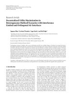
5.2. STTBCS: Structure and Algorithm. We apply the pro-
posed TBCS to UWB systems to develop the STTBCS algo-
rithm. Figure 4 illustrates the structure of our STTBCS algo-
rithm and explains how mutual information is exchanged.
For simplicity, only two b ase stations (BS1 and BS2) and two
consecutive fr ames of UWB signals (the kth and (k + 1)th)
in each base station are illustrated. For each BCS procedure,
Figure 4 also depicts the dependence among measurements,
noise, signal elements, and hyperparameters.
In the STTBCS, multiple BCS procedures in multiple
time slots are performed. Between BS1 and BS2, the signal
reconstruction for s
1(k+1)
and s
2(k+1)
is carried out simulta-
neously while the information in s

1k
and s
2k
, the previous
frame, is also used.
Algorithm 1 shows the details of the STTBCS algorithm.
We start with the initialization of the noise, hyperparameters
α, and the candidate index set Ω (an index set containing
all possibly nonzero element indices). Then, the information
EURASIP Journal on Advances in Signal Processing 9
(1) The hyperparameter α is set to α = [∞, , ∞].
The candidate index set Ω
=∅.
The noise is initialized to a certain value without any prior information, or utilize
the previous estimated value.
The parameter of the hyperparameter λ : λ
= [0, 0];
(2) Update λ using (11) and (13) from the previous reconstructed nonzero signal elements.
This introduces temporal aprioriinformation.
(3) repeat
(4) Check and receive the ongoing reconstructed signal elements from other simultaneous
BCS reconstruction procedures to update the parameter. λ; this is to fuse spatial apriori
information.
(5) Choose a random jth index; Calculate the corresponding parameter g
j
and h
j
as shown
in (C.4) and (C.5).
(6) if (g

j
)
2
>h
j
and

λ
j
/
=0 then
(7) Add a candidate index: Ω
= Ω ∪ j;
(8) Update α
j
by solving (24).
(9) else
(10) if (g
j
)
2
>h
j
and

λ
j
= 0 then
(11) Add a candidate index: Ω
= Ω ∪ j

(12) Update α
i
using (23).
(13) else if (g
j
)
2
<h
j
then
(14) Delete the candidate index: Ω
= Ω \{j} if the index is in the candidate set.
(15) end if
(16) end if
(17) Compute the signal coefficients s
Ω
in the candidate set using (5).
(18) Send out the ongoing reconstructed signal elements s
Ω
to other BCS procedures
as spatial aprioriinformation.
(19) until converged
(20) Re-estimate the noise level using (28) and send out the noise level for the next usage.
(21) Send out the reconstructed nonzero signal elements for the next time utilization as
temporal aprioriinformation.
(22) Return the reconstructed signal.
Algorithm 1: Space-time tur bo bayesian compressed sensing algorithm.
from previous reconstructed signals and from other base
stations is utilized to update the hyperparameter λ. The terms
g

j
and h
j
are also computed. The term g
2
j
>h
j
is then
used to add the jth element from the candidate index set. A
convergence criterion is used to test whether the differences
between successive values for any α
j
, j ={1, 2, , N} are
sufficiently small compared to a certain threshold. When the
iterations are completed, the noise level β will be reestimated
from setting ∂L/∂β
= 0 using the same method in [21], which
is given by

β
2

new
=


y −ΣS



2
N −

M
i=1
(
1
− α
i
Σ
ii
)
,
(28)
where Σ
ii
is the diagonal element in the matrix Σ.The
details of the above STTBCS algorithm are summarized
in Algorithm 1. Note that only the nonzero signal element
which is shown from the local measurements can introduce
aprioriinformation and thus update the hyperparameter

λ
j
.
In other words, only if it satisfies g
2
j
>h
j

can the parameter

λ
j
be updated. This avoids the adverse effects from wrong
aprioriinformation to add a zero signal element into the
candidate index set.
6. Simulation Results
Numerical simulations are conducted to evaluate the per-
formance of the proposed TBCS algorithm, compared with
the MBCS [23] and original BCS algorithms [5]. We use
spike signals and experimental UWB echo signals [26]for
the performance test. The quality of the reconstructed signal
10 EURASIP Journal on Advances in Signal Processing
ββ
ββ
y
1(k+1)
λ
1(k+1)
α
1(k+1)
y
2(k+1)
λ
2(k+1)
α
2(k+1)
Parallel Parallel
Serial

Serial
s
2(k+1)
s
1(k+1)
y
1k
s
1k
α
1k
λ
1k
BS1
y
2k
s
2k
α
2k
λ
2k
BS2
Time
Space
Figure 4: Block diagram of space-time turbo Bayesian compressed sensing.
is measured in terms of the reconstruction percentage, which
is defined as
1
−



s −s


2
s
2
,
(29)
where s is the true signal and
s is the reconstructed signal.
Our TBCS algorithm performance is largely determined
by how the int roduced signal is similar to the objective signal.
In other words, we consider how many common nonzero
element locations are shared between the objective signal and
the introduced signals. Then we define the similarity as
P
s
=
K
com
K
obj
,
(30)
where K
obj
is the number of nonzero signal elements in
the objective unrecovered signal, K

com
is the number of the
common nonzero element locations among the transferred
reconstructed signals and objective signal, and P
s
represents
the similarity level as a percentage. Note that, without
loss of generality, we only consider the relative number
of common nonzero element locations to measure the
similarity, ignoring any amplitude correlation. Hence, when
P
s
= 100%, it does not mean that the signals are the same but
means that they have the same nonzero element locations;
the amplitudes may not be the same.
Our TBCS algorithm performance is compared with
MBCS and BCS using different types of signals, different
similarity levels, noise powers, and measurement numbers.
6.1. Spike Signal. We first generate four scenarios of spike
signals with the same length N
= 512, which have the
same number of 20 nonzero signal elements with random
locations and Gaussian distributed (mean
= 0, variance =
1) amplitudes. One spike signal is selected as the objective
signal, as shown in Figure 5. With respect to the objective
signal, the other three signals have a similarity of 25%, 50%,
and 75%, which will be introduced as aprioriinformation.
50 100 150 200 250 300 350 400 450 500
−3

−2.5
−2
−1.5
−1
−0.5
0
0.5
1
1.5
2
Figure 5: Spike signal with 20 nonzero elements in random
locations.
50 100 150 200 250 300 350 400 450 500
−3
−2.5
−2
−1.5
−1
−0.5
0
0.5
1
1.5
2
Figure 6: Reconstructed spike signal using MBCS w ith 75%
similarity.
The objective signal is then reconstructed using the original
BCS, MBCS, and TBCS algorithms, respectively, with the
same number of measurements (M
= 62) and the same

noise variance 0.15 (SNR
 6 dB). We also investigate the
performance gain (in terms of reconstruction percentage) at
each iteration.
EURASIP Journal on Advances in Signal Processing 11
50 100 150 200 250 300 350 400 450 500
−3
−2.5
−2
−1.5
−1
−0.5
0
0.5
1
1.5
2
Figure 7: Reconstructed spike signal using TBCS with 75%
similarity.
Figures 6 and 7 show the reconstructed spike signal
using MBCS and TBCS, respectively, by introducing the
spike signal with a similarity of 75%. The reconstruction
percentage using TBCS is 92.7% while it is 57.5% using
MBCS. The comparison of the two figures shows that TBCS
can recover most of the original signal while MBCS fails to
reconstruct the signal with so few measurements (M
= 62) in
spite of using a high-similarity signal as aprioriinformation.
Figures 8, 9,and10 show, when transferred signals
have a similarity of 25%, 50%, and 75%, respectively, how

much signal reconstruction percentage can be achieved at
each iteration using the BCS, MBCS, and TBCS algor ithms.
The simulations are run 100 times, over w h ich the results
are averaged. It is clear that our proposed TBCS is much
better than the BCS at each iteration. Particularly, when the
similarity is 25%, MBCS is worse than BCS while our TBCS
achieves higher performance at each iteration than BCS. For
instance, at iteration 25 in Figure 8, TBCS can achieve a
reconstruction percentage of 61.7%, while BCS can reach
42.2% and MBCS only recovers 35.6%. It shows that, at a
low similarity, our TBCS can still achieve good performance
at every iteration, compared with MBCS and BCS. Moreover,
with a high similarity, the performance gap between TBCS
and MBCS is enlarged at each step. For example, at iteration
21 with a similarity of 25% in Figure 8, TBCS can achieve
a reconstruction percentage of 59.7%, while MBCS can
reach 28.2%. Hence, the performance gap is 31.5%. When
the similarity is 75% in Figure 10, the performance gap is
increased to 50.9% because TBCS can reach 80.5%, while
MBCS achieves 29.6% at the 21st iteration.
6.2. UWB Signal. The tested scenarios are the experimental
UWB echo pulses from various UWB propagation channels
in practical indoor residential, office, and clean, line-of-
sight (LOS) and non-line-of-sight (NLOS) environments,
which are drawn from experimental IEEE 802.15.4a UWB
propagation models [26]. In a typical UWB communica-
tion/positioning system where receivers are distributed in the
same environment, the received UWB echo signals are more
or less similar. We test performance of original BCS, TBCS,
and MBCS algorithms with different similarity levels.

5 1015202530
−0.2
0
0.2
0.4
0.6
0.8
1
Iteration
Original BCS
TBCS
MBCS
Reconstruction (%)
Figure 8: Performance gain in each iteration with 25% similarity.
5 1015202530
−0.2
0
0.2
0.4
0.6
0.8
1
Iteration
Original BCS
TBCS
MBCS
Reconstruction (%)
Figure 9: Performance gain in each iteration with 50% similarity.
5 1015202530
−0.2

0
0.2
0.4
0.6
0.8
1
Iteration
Original BCS
TBCS
MBCS
Reconstruction (%)
Figure 10: Performance gain in each iteration with 75% similarity.
Figure 11 shows the reconstructed UWB echo signals
using the orig inal BCS and our TBCS algorithms. The test
UWB echo signals S0 (not shown in Figure 11), S1, S2, S3,
12 EURASIP Journal on Advances in Signal Processing
50 100 150
−1
0
1
(a) BCS reconstructed S1: 81.2%
50 100 150
−1
0
1
(b) TBCS reconstructed S1: 84.4%
50 100 150
50 100 150
−1
0

1
(c) BCS reconstructed S2: 46.4%
50 100 150
1
0
1
(d) TBCS reconstructed S2: 89.7%
50 100 150
−1
0
1
(e) BCS reconstructed S3: 14.9%
50 100 150
−1
0
1
(f) TBCS reconstructed S3: 92.8%
50 100 150
−1
0
1
(g) BCS reconstructed S4: −77%
50 100 150
−1
0
1
(h) TBCS reconstructed S4: 93.2%
Figure 11: The performance of original BCS and TBCS. The UWB echo signals S1, S2, S3, and S4 with length N = 512 are reconstructed
using the BCS and TBCS algorithms but only a section (length
= 150) is shown. In the TBCS algorithm, the reconstructed signal S0

(not shown) is transferred to other signal reconstruction as aprioriinformation. The number of measurements, SNR, similarity, and
reconstruction percentage are (a) and (b) measurements M
= 60; SNR = 9.2 dB; with respect to S0, the similarity in S1 is 11.5%; the
reconstruction percentages of S1 using BCS and TBCS algorithms are 81.2% and 84.4%, respectively. (c) and (d) M
= 60, SNR = 17.7 dB;
with respect to S0, similarity in S2 is 31.3%; the reconstruction percentages are 46.4% and 89.7%. (e) and (f) M
= 50, SNR = 12.4 dB; 61.0%
similarity; the reconstruction percentages are 14.9% and 92.8%. (g) and (h) M
= 70, SNR = 15.1 dB; 98.1% similarity; the reconstruction
percentages are
−77.0% and 93.2%.
and S4 are drawn from the IEEE802.15 UWB propagation
model [26], in which the reconstructed S0asapriori
information is transferred to the other four signal scenarios.
With respect to S0, the similarity levels in S1, S2, S3, and
S4 are 11.5%, 31.3%, 61.0%, and 98.1%, respectively. For
each signal, both algorithms utilize the same number of
measurements with the same SNR level for reconstruction.
For clarity, only a portion of the UWB signal scenario
is expanded to illustrate the waveform details of the
reconstructed pulses. It is clearly observed from Figure 11
EURASIP Journal on Advances in Signal Processing 13
40 50 60 70 80 90 100 110 120 130
0
0.1
0.2
0.3
0.4
0.5
0.6

0.7
0.8
0.9
1
Number of measurements
Original BCS
TBCS, 16.6% similarity
MBCS, 16.6% similarity
TBCS, 66.1% similarity
MBCS, 66.1% similarity
Reconstruction (%)
Figure 12: Performance comparison at different similarity levels
without noise.
60 70 80 90 100 110 120 130 140 150 160
0
0.1
0.2
0.3
0.4
0.5
0.6
0.7
0.8
0.9
Number of measurements
Original BCS
TBCS, 16.6% similarity
MBCS, 16.6% similarity
TBCS, 66.1% similarity
MBCS, 66.1% similarity

Reconstruction (%)
Figure 13: Performance comparison at different similarity levels in
the presence of noise.
that our TBCS is much better than the original BCS for
different similarity levels. The reconstruction percentages
using TBCS are much higher than those using original BCS
by introducing aprioriinformation with the same number of
measurements. Moreover, the performance gap is increasing
with the growth of the similarity level. For instance, with a
similarity of 11.5% for reconstructing the signal S1 in Figures
11(a) and 11(b), the difference of reconstruction percentages
using BCS and TBCS is only 3.2% (84.4–81.2%). When the
similarity level is 98.1% for reconstructing the signal S4in
Figures 11(g) and 11(h), the difference is increased to 170.2%
(93.2–(
−77%)). Therefore, with a higher similarity level,
higher performance gain can be achieved.
The perform ance of the original BCS, MBCS, and TBCS
at different similarity levels is then compared. We select
three UWB echo signals S5, S6, and S7 with the same
dimension N
= 512. The additive noise variance is only
0.01, implying a very high SNR. The reconstructed signals
−5 0 5 101520253035
10
−3
10
−2
10
−1

10
0
SNR
Bit error rate
Original BCS
TBCS, 16.6% similarity
MBCS, 16.6% similarity TBCS, 66.1% similarity
MBCS, 66.1% similarity
Figure 14: BER performance using different algorithms.
S6andS7asaprioriinformation are transferred to the
signal reconstruction for S5. With respect to S6andS7,
the similarities in S5 are 16.3% and 64.4%, respectively.
The signal S5 is recovered with different numbers of
measurements using the original BCS, TBCS, and MBCS
algorithms. Figure 12 shows the reconstruction percentages
versus the number of measurements for the signal S5.
Obviously, at a low similarity level, the MBCS performance
is substantially worse than the orig inal BCS whereas our
TBCS achieves a performance equaling that of the original
BCS performance. For a high similarity level, both MBCS
and TBCS are much better than the original BCS due to
the benefits of high similarity transferred from the signal S7.
This demonst rates that our TBCS achieves a good balance
between local observations and aprioriinformation, leading
to a more robust performance than the MBCS.
In the presence of more noise interference, our TBCS
still outperforms MBCS and BCS, as shown in Figure 13.We
use the same signals S5, S6, and S7 but the noise variance
is increased to 0.4. We observe that our TBCS exhibits
good performance, as shown in Figure 12. Particularly in the

presence of noise, when the number of measurements is large
enough (M>150). At a low similarity level, the MBCS
can achieve a maximum reconstruction percentage of 74.5%
while our TBCS algorithm is able to accomplish a maximum
reconstruction percentage of 86.9%. At a high similarity
level, MBCS can reach a maximum of 80.1% while our TBCS
algorithm is still able to accomplish a maximum of 86.9%.
Therefore, by introducing aprioriinformation, the proposed
TBCS algorithm can significantly reduce the number of mea-
surements and improve the capability of combating noise.
Figure 14 shows the Bit Error Rate (BER) for an example
UWB communication system using different algorithms.
We utilize Binary Phase Shift Keying (BPSK) modulation
to transfer the data since biphase modulation is one of
the easiest methods to implement. The performance of the
TBCS, MBCS, and the original BCS algorithms is compared
for the UWB communication system. The BER is tested using
different noise levels with the same number of measurements
(M
= 112). With so few measurements, using the BCS
algorithm leads to a high BER at different SNR. It is
14 EURASIP Journal on Advances in Signal Processing
also observed that, at a low similarity level, the TBCS
performance is much better than the MBCS algorithm. At
a high similarity level, the BER per formance using the TBCS
and MBCS algorithms are much better than that using the
original BCS algorithm, while TBCS is the best. Therefore, by
applying our TBCS algorithm in the UWB communication
system, it can reduce the BER, provide more tolerance of the
noise, and thus achieve the best performance when compared

with the MBCS and BCS algorithms.
7. Conclusion
This paper has proposed an efficient approach to exploit and
integrate the spatial and temporal aprioriinformation exist-
ing in sparse signals, for example, UWB pulses. The turbo
BCS algorithm has been designed to fully exploit apriori
information from both space and time. Numerical simula-
tion results have shown that the proposed TBCS outperforms
the MBCS and traditional BCS, in terms of the robustness to
noise and reduction of the required amount of samples.
Appendices
A. Proof of (9) and (10)
We first show the derivation of (9), which is given by
P

s
i
j
| λ
i
j

=

P

s
i
j
| α

i
j

P

α
i
j
| λ
i
j

dα
i
j
=

⎛
⎝
α
i
j
2π
⎞
⎠
−(1/2)
exp
⎛
⎜
⎝

−

s
i
j

2
α
i
j
2
⎞
⎟
⎠
λ
i
j
exp

−
λ
i
j
α
i
j

dα
i
j

=
λ
i
j
(
2π
)
1/2


α
i
j

−(1/2)
exp
⎛
⎜
⎝
−
⎛
⎜
⎝
λ
i
j
+

s
i

j

2
2
⎞
⎟
⎠
α
i
j
⎞
⎟
⎠
dα
i
j
.
Let
t
=
⎛
⎜
⎝
λ
i
j
+

s
i

j

2
2
⎞
⎟
⎠
α
i
j
=
λ
i
j
(
2π
)
1/2

⎛
⎜
⎜
⎝
t
λ
i
j
+



s
i
j

2
/2

⎞
⎟
⎟
⎠
1/2
exp
(
−t
)
,
d
⎛
⎜
⎜
⎝
t
λ
i
j
+


s

i
j

2
/2

⎞
⎟
⎟
⎠
=
λ
i
j
(
2π
)
1/2
⎛
⎜
⎝
λ
i
j
+

s
i
j


2
2
⎞
⎟
⎠
−(3/2)

t
1/2
exp
(
−t
)
dt
=
(
2π
)
−(1/2)
Γ

3
2

λ
i
j
⎛
⎜
⎝

λ
i
j
+

s
i
j

2
2
⎞
⎟
⎠
−(3/2)
,
(A.1)
where Γ(
·) is the gamma function, defined as Γ(x) =

∞
0
t
x−1
e
−t
dt.WehaveΓ(3/2) =

∞
0

t
1/2
e
−t
dt. Because both
distributions belong to the exponential distribution family,
the marginal distribution is still in the same family. It is also
observed that the marginal distribution P(s
i
j
| λ
i
j
) is sharply
peaked at zero, which encourages the sparsity. Therefore, the
chosen exponential a prior distribution in the hierarchical
Bayesian framework can be recognized and encourage the
sparsity of the reconstructed signal.
Based on the assumption α
b
j
= α
i
j
, we have the same
derivation:
P

s
b

j
| λ
i
j

=

P

s
b
j
| α
i
j

P

α
i
j
| λ
i
j

dα
i
j
=


⎛
⎝
α
i
j
2π
⎞
⎠
−(1/2)
exp
⎛
⎜
⎝
−

s
b
j

2
α
i
j
2
⎞
⎟
⎠
λ
i
j

exp

−
λ
i
j
α
i
j

dα
i
j
=
(
2π
)
−(1/2)
Γ

3
2

λ
i
j
⎛
⎜
⎝
λ

i
j
+

s
b
j

2
2
⎞
⎟
⎠
−(3/2)
.
(A.2)
Inordertoobtain(10), we utilize the above e quations. Then
the derivation of the posterior is given by
P

α
i
j
| s
b
j
, λ
i
j


=
P

s
b
j
| α
i
j

P

α
i
j
| λ
i
j

P

s
b
j
, λ
i
j

=
P


s
b
j
| α
i
j

P

α
i
j
| λ
i
j


P

s
b
j
| α
i
j

P

α

i
j
| λ
b
j

dα
i
j
=

α
i
j

−1
(
2π
)
−(1/2)
λ
i
j
exp

−


s
b

j

2
α
i
j
/2

−
α
i
j
λ
i
j

(
2π
)
−(1/2)
Γ
(
3/2
)

λ
i
j
+



s
b
j

2
/2

−(3/2)
λ
i
j
=

λ
i
j
+


s
b
j

2
/2

3/2
exp


−

λ
i
j
+

s
b
j

2
/2

α
i
j

Γ
(
3/2
)
=


λ
i
j

3/2

exp

−

λ
i
j
α
i
j

Γ
(
3/2
)
.
(A.3)
So the parameter λ
i
j
is updated to

λ
i
j
, which is given by

λ
i
j

= λ
i
j
+

s
b
j

2
2
.
(A.4)
EURASIP Journal on Advances in Signal Processing 15
For transferred multiplied reconstructed signal elements
s
b
1
j
, s
b
2
j
, s
b
n
j
, the posterior function also belongs to the
exponential distribution family. As shown in (12 ), the
parameter λ

i
j
is updated to
P

α
i
j
| s
b
1
j
, s
b
2
j
, , s
b
n
j
, λ
i
j

=
P

s
b
1

j
| α
i
j

P

s
b
2
j
| α
i
j

···
P

s
b
n
j
| α
i
j

P

α
i

j
| λ
i
j

P

s
b
1
j
, s
b
2
j
, , s
b
n
j
, λ
i
j

=
P

s
b
1
j

| α
i
j

P

s
b
2
j
| α
i
j

···
P

s
b
n
j
| α
i
j

P

α
i
j

| λ
i
j


P

s
b
1
j
, α
i
j
| λ
i
j

P

s
b
2
j
, α
i
j
| λ
i
j


···
P

s
b
n
j
, α
i
j
| λ
i
j

dα
i
j
=
P

s
b
1
j
| α
i
j

P


s
b
2
j
| α
i
j

···
P

s
b
n
j
| α
i
j

P

α
i
j
| λ
i
j



P

s
b
1
j
| α
i
j
, λ
i
j

P

s
b
2
j
| α
i
j
, λ
i
j

···
P

s

b
n
j
| α
i
j
, λ
i
j

P

α
i
j
| λ
i
j

dα
i
j
=

λ
i
j
+
n


i=1

s
b
i
j

2
/2

(2n+1)/2
exp

−

λ
i
j
+

n
i=1

s
b
i
j

2
/2


α
i
j

Γ
((
2n +1
)
/2
)
=


λ
i
j

(2n+1)/2
exp

−

λ
j
α
i
j

Γ

((
2n +1
)
/2
)
.
(A.5)
The distributions P(s
b
1
j
α
i
j
), P(s
b
2
j
α
i
j
), ,andP(s
b
n
j
| α
i
j
)
are conditionally independent from each other. In this case,

the parameter is updated to

λ
i
j
= λ
i
j
+

n
i=1

s
b
i
j

2
2
,
(A.6)
where n represents the total number of aprioriinformation
s
b
1
j
, s
b
2

j
, s
b
n
j
.
Therefore, the above derivations show how the single or
multiple signal elements s
b
n
j
, j = 1, 2, , N, n = 1, 2, ,
from the other BCS procedures update the hyperparameters
in the ith BCS signal reconstruction procedure.
B. Derivation of (15)
One strategy to maximize (17) is to exploit an EM method,
treating the s
i
as hidden data, and maximize the fol l owing
expectation:
E
s
i
|y
i
,α
i

log P


s
i
| α
i

P

α
i
| λ
i

. (B.1)
The operator E
s
i
|y
i
,α
i
denotes an expectation of the
posterior P(s
i
| y
i
, α
i
, λ
i
, β) with respect to the distribution

over the s
i
given the data and hidden variables. Through
differentiation with respect to α
i
we get
∂
∂α
i
j
E
s
i
|y
i
,α
i

log P

s
i
| α
i
, β

P

α
i

| λ
i

=
E
s
i
|y
i
,α
i
⎡
⎣
∂
∂α
i
j

log P

s
i
| α
i
, β

+logP

α
i

| λ
i

⎤
⎦
=−
1
2
E
s
i
|y
i
,α
i
⎡
⎣
−
2

s
i
j

2
− 4λ
i
j
+
6

α
i
j
⎤
⎦
=
E
s
i
|y
i
,α
i


s
i
j

2

+2λ
i
j
−
3
α
i
j
.

(B.2)
According to (3), we have
E
s
i
|y
i
,α
i


s
i
j

2

=
Σ
i
jj
+

μ
i
j

2
. (B.3)
We set (B.2) to 0, which yields an update for α

i
j
:
α
i
j
=
3

s
i
j

2
+ Σ
i
jj
+2λ
i
j
.
(B.4)
C. Derivation of (19)
For the L
1
(α), as shown in [21], we have that
L
1
(
α

)
=−
1
2

N log 2π +log|E| + y
T
E
−1
y

=
L
1

α
−j

+ l
1

α
j

,
(C.1)
where,
E
= σ
2

I + ΦA
−1
Φ
T
= σ
2
I +

k
/
= j
α
−1
k
φ
k
φ
−1
k
+ α
−1
j
φ
j
φ
j
= E
−j
+ α
−1

j
φ
j
φ
j
,
(C.2)
L
1
(
α
−i
)
=−
1
2

N log 2π +log



E
−j



+ y
T
E
−1

−j
y

,
l
1

α
j

=
1
2

log α
j
− log

α
j
+ g
j

+
h
2
j
α
j
+ g

j

.
(C.3)
The quantities g
j
, h
j
,andE
−j
are given by
g
j
= φ
T
j
E
−1
−j
φ
j
,
(C.4)
h
j
= φ
T
j
E
−1

−j
y,(C.5)
E
−j
= β
2
I +

k
/
= j
α
−1
k
φ
k
φ
−1
k
,
(C.6)
where φ
j
is the jth column vector of the matrix Φ.
16 EURASIP Journal on Advances in Signal Processing
In order to find the critical point, the differentiation of
l
1
(α
j

)isgivenby
∂l
1

α
j

∂α
j
=
α
−1
j
g
2
j
−

h
2
j

+ g
j
2

α
j
+ g
j


2
= 0.
(C.7)
It is easy to maximize l
1
(α
j
)withrespecttoα
j
by taking the
first and second derivatives. Then the maximum point α
j
is
given by
α

j
=
⎧
⎪
⎪
⎨
⎪
⎪
⎩
h
2
j
g

2
j
− h
j
,ifg
2
j
>h
j
,
∝, otherwise.
(C.8)
The second derivative is
∂
2
l
1

α
j

∂α
2
j
=
−
2α
2
j


α
j
+ g
j

α
−1
j
g
2
j
− h
2
j
+ g
j

−

α
j
+ g
j

2
g
2
j
2α
2

j

α
j
+ g
j

4
.
(C.9)
Taking the critical point α

j
into the second derivative
expression, we have known that
∂
2
l
1

α
j
= α

j

∂α
2
j
=

−
g
2
j
2α
2
j

α
j
+ g
j

2
.
(C.10)
Obviously, it is always negative, and therefore function l
1
(α
j
)
achieves the maximum at α

j
, which is unique.
D. Derivations about (24) and (25)
The first derivative of the l
2
(α
j

)isl

2
(α
j
) =−λ
j
. All together
the first differentiation of the posterior l(α
j
)isgivenby
l


α
j

=
l

1

α
j

+ l

2

α

j

=
⎛
⎜
⎝
g
j
2α
j

α
j
+ g
j

−
h
2
j
2

α
j
+ g
j

2
⎞
⎟

⎠
−
λ
j
=
1
2
⎡
⎢
⎣
1
α
j
−
1
α
j
+ g
j
−
h
2
j

α
j
+ g
j

2

− 2λ
j
⎤
⎥
⎦
.
(D.1)
By setting the (D.1) to zero, we can find the optimum α

j
for
(25).
The g
j
and h
2
j
are not negative based on (C.4)and(C.5).
We have α
j
≥ 0andλ
j
> 0 according to the exponential
distribution as shown in (7), and l

(α
j
) →−2λ
j
< 0asα

j
→
+∞. Then, it has l

(α
j
) > 0 when α
j
→ 0. Therefore, for the
function l

(α
j
) = 0, it has at least one positive root for α
j
> 0.
We rear ra nge (D.1)to
l


α
j

=
1
2
⎡
⎢
⎣
1

α
j
−
1
α
j
+ g
j
−
h
2
j

α
j
+ g
j

2
− 2λ
j
⎤
⎥
⎦
=
f

α
j
, g

j
, h
j
, λ
j

α
j

α
j
+ g
j

2
.
(D.2)
Setting (D.2) to zero is to let the numerator be zero, that
is, f (α
j
, g
j
, h
j
, λ
j
) = 0. To find the solution, we normalize the
equation to reduce one parameter for convenienc e. Then we
need to solve
f


α
j
, g
j
, h
j
, λ
j

−2λ
j
= α
3
j
+ B
0
α
2
j
+ B
1
α
j
+ B
2
= 0.
(D.3)
The corresponding coefficients are given by [31]
B

0
= 2g
j
,
B
1
=
g
j
− 2λ
j
g
2
j
− h
2
j
−2λ
j
,
B
2
=
g
2
j
−2λ
j
.
(D.4)

To solve the cubic function, we define intermediate
components as
U
= 2B
3
0
− 9B
0
B
1
+27B
2
,
V
=

2B
3
0
− 9B
0
B
1
+27B
2

2
− 4

B

2
0
− 3B
1

3
.
(D.5)
Then the solutions of the cubic function are given by
x
1
=−
1
3
⎛
⎝
B
0
+
3

U +
√
V
2
+
3

U −
√

V
2
⎞
⎠
,
x
2
=−
1
3
⎛
⎝
B
0
+ ω
1
3

U +
√
V
2
+ ω
2
3

U −
√
V
2

⎞
⎠
,
x
3
=−
1
3
⎛
⎝
B
0
+ ω
2
3

U +
√
V
2
+ ω
1
3

U −
√
V
2
⎞
⎠

,
(D.6)
where,
ω
1
=−
1
2
+
√
3
2
i
ω
2
=−
1
2
−
√
3
2
i.
(D.7)
Therefore, all those three roots x
1
, x
2
,andx
3

are cr itical
points of the optimization function shown in (19). We
choose the positive root which maximizes the optimization
function in (19) as the optimum solution α
∗
j
for (25).
References
[1] D. L. Donoho, “Compressed sensing,” IEEE Transactions on
Information Theory, vol. 52, no. 4, pp. 1289–1306, 2006.
[2] E. J. Cand
`
es, J. Romberg, and T. Tao, “Robust uncertainty
principles: exact signal reconstruction from highly incomplete
frequency information,” IEEE Transactions on Information
Theory, vol. 52, no. 2, pp. 489–509, 2006.
[3] H. Zayyani, M. Babaie-Zadeh, and C. Jutten, “Bayesian pursuit
algorithm for sparse representation,” in Proceedings of the
IEEE International Conference on Acoustics, Speech, and Signal
Processing (ICASSP ’09), pp. 1549–1552, Taipei, Taiwan, April
2009.
EURASIP Journal on Advances in Signal Processing 17
[4] H. Zayyani, M. Babaie-Zadeh, and C. Jutten, “An iterative
Bayesian algorithm for sparse component analysis in presence
of noise,” IEEE Transactions on Signal Processing, vol. 57, no.
11, pp. 4378–4390, 2009.
[5] S. Ji, Y. Xue, and L. Carin, “Bayesian compressive sensing,”
IEEE Transactions on Signal Processing, vol. 56, no. 6, pp. 2346–
2356, 2008.
[6] D. Yang, H. Li, G. D. Peterson, and A. Fathy, “Compressed

sensing based UWB receiver: hardware compressing and
FPGA reconstruction,” in Proceedings of the 43rd Annual
Conference on Information Sciences and Systems (CISS ’09),pp.
198–201, Baltimore, Md, USA, March 2009.
[7] Z.Wang,G.R.Arce,B.M.Sadler,J.L.Paredes,S.Hoyos,and
Z. Yu, “Compressed UWB signal detection with narrowband
interference mitigation,” in Proceedings of the IEEE Interna-
tional Conference on Ultra-Wideband (ICUWB ’08), pp. 157–
160, Singapore, September 2008.
[8] D. Yang, H. Li, and G. D. Peterson, “Feedback orthogonal
pruning pursuit for pulse acquisition in UWB communi-
cations,” in Proceedings of the 20th IEEE Personal, Indoor
and Mobile Radio Communications Symposium (PIMRC ’09),
Tokyu, Japapn, September 2009.
[9] P. Zhang, Z. Hu, R. C. Qiu, and B. M. Sadler, “Compressive
sensing based ultra-wideband communication system,” in
Proceedings of the IEEE International Conference on Commu-
nications (ICC ’09), Dresden, Germany, June 2009.
[10] D. Baron, M. B. Wakin, M. F. Duarte, S. Sarvotham, and R. G.
Baraniuk, “Distributed compressed sensing,” available online,
/>[11] W. Wang, M. Garofalakis, and K. Ramchandran, “Distributed
sparse random projections for refinable approximation,” in
Proceedings of the 6th International Symposium on Information
Processing in Sensor Networks (IPSN ’07), pp. 331–339, Cam-
bridge, Mass, USA, April 2007.
[12] D. Leviatan and V. N. Temlyakov, “Simultaneous approxima-
tion by greedy algorithms,” IMI Report 2003, University of
South Carolina at Columbia, 2003.
[13] J. A. Tropp, A. C. Gilbert, and M. J. Strauss, “Algorithms for
simultaneous sparse approximation. Part I: greedy pursuit,”

Signal Processing, vol. 86, no. 3, pp. 572–588, 2006.
[14] N. Vaswani and W. Lu, “Modified-CS: modifying compressive
sensing for problems with partially known support,” in Pro-
ceedings of the IEEE International Symposium on Information
Theory (ISIT ’09), pp. 488–492, Seoul, Korea, July 2009.
[15] E. Berg and M. P. Friedlander, “Joint-sparse recovery
from multiple measurements,” available online, http://www
.arxiv.org/abs/0904.2051v1.
[16] F. Zhang and H. D. Pfister, “On the iterative decoding
of highrate LDPC codes with applications in compressed
sensing,” available online, />[17] X. Tan and J. Li, “Computationally efficient sparse Bayesian
learning via belief propagation,” IEEE Transactions on Signal
Processing, vol. 58, no. 4, pp. 2010–2021, 2010.
[18] D. Baron, S. Sar votham, and R. G. Baraniuk, “Bayesian
compressive sensing via belief propagation,” IEEE Transactions
on Signal Processing, vol. 58, no. 1, pp. 269–280, 2010.
[19] P. Schniter, L. C. Potter, and J. Ziniel, “Fast Bayesian matching
pursuit,” in Proceedings of the Information Theory and Appli-
cations Workshop (ITA ’08), pp. 326–332, La Jolla, Calif, USA,
January-February 2008.
[20] S. D. Babacan, R. Molina, and A. K. Katsaggelos, “Bayesian
compressive sensing using laplace priors,” IEEE Transactions
on Image Processing, vol. 19, no. 1, pp. 53–63, 2010.
[21] M. E. Tipping, “Sparse Bayesian learning and the relevance
vector machine,” Journal of Machine Learning Research, vol. 1,
no. 3, pp. 211–244, 2001.
[22] D. Yang, H. Li, G. D. Peterson, and A. E. Fathy, “UWB
signal acquisition in positioning systems: Bayesian compressed
sensing with redundancy,” in Proceedings of the 43rd Annual
Conference on Information Sciences and Systems (CISS ’09),pp.

192–197, Baltimore, Md, USA, March 2009.
[23] S. Ji, D. Dunson, and L. Carin, “Multitask compressive sens-
ing,” IEEE Transactions on Signal Processing,vol.57,no.1,pp.
92–106, 2009.
[24] Y. Qi, D. Liu, D. Dunson, and L. Carin, “Bayesian multi-task
compressive sensing with dirichlet process priors,” in Interna-
tional Conference on Machine Learning, Helsinki, Finland, July
2008.
[25] M. E. Tipping and A. C. Faul, “Fast marginal likelihood
maximisation for sparse Bayesian models,” in Proceedings
of the International Conference on Artific ial Intelligence and
Statistics, Key West, Fla, USA, June 2003.
[26] A. F. Molisch et al., “IEEE 802.15.4a channel model—final
report,” IEEE 2004, />04-0662-02-004a-channel-model-final-report-r1.pdf.
[27] A.Gelman,J.B.Carlin,H.S.Stern,andD.B.Rubin,Bayesian
Data Analysis, CRC Press, New York, NY, USA, 2nd edition,
2003.
[28] D. Yang, G. D. Peterson, H. Li, and J. Sun, “An FPGA
implementation for solving least square problem,” in Proceed-
ings of the IEEE Symposium on Field Programmable Custom
Computing Machines (FCCM ’09), pp. 303–306, Napa, Calif,
USA, April 2009.
[29] D. Yang, G. Peterson, and H. Li, “High performance recon-
figurable computing for Cholesky decomposition,” in Pro-
ceedings of the Symposium on Application Accelerators in High
Performance Computing (UIUC ’09), Urbana, Ill, USA, July
2009.
[30] D. Yang, A. Fathy, H. Li, G. D. Peterson, and M. Mahfouze,
“Millimeter accuracy UWB positioning system using sequen-
tial sub-sampler and time difference estimation algorithm,”

in Proceedings of the IEEE Radio and Wireless Symposium
(RWS ’10), New Orlean, Fla, USA, January 2010.
[31] W. S. Anglin and J. Lambek, The Heritage of Thales, Springer,
New York, NY, USA, 1993.