Solar Collectors and Panels, Theory and Applicationsband (CTB) Part 5 ppt

Solar Collectors and Panels, Theory and Applications

112
positively charged helium nuclei; and iii) beta particles, rapidly moving electrons. The
artificial radioactive elements are formed by bombardment with high energy particles such
as helium nuclei. The most of the radiation in ultraviolet region of radiation spectrum is
absorbed by the ozone in the upper atmosphere, whilst part of the radiation in the
shortwave region of the radiation spectrum is scattered by air molecules, for communication
of blue colour appearance of sky to our eyes. The strength of the absorption of solar energy
varies with wavelength and absorption bands are formed at regions of strong absorption.
The important atmospheric gases forming part of absorption bands are ozone (O
3
), water
vapour (H
2
O), carbon dioxide (CO
2
), oxygen (O
2
), methane (CH
4
), chlorofluorocarbons
(CFC) and nitrogen dioxide (NO
2
).
The scope of the chapter is to present detailed theoretical aspects of solar energy absorbers,
their radiation properties, radiation sources, diffraction and measurement of radiation
sources. The importance of selection of roughness factors based on fluid flow is pointed out.
The human environmental health is presented for metabolism of your body to intense solar
radiation and heat. Mathematical analysis of a solar thermosyphon and experimental results

for applications of solar collectors to the environment, human health and buildings are
elaborated later in the chapter.
2. Theory
The rate of electromagnetic radiation emitted at a rate E
x
from the surface of a solar energy
absorber is given by the Stefan-Boltzmann equation as follows:
E
x
= εσT
4
(1)
Where, E
x
is exitance of a solar energy absorber, T is temperature in K, σ is Stefan-Boltzmann
constant, 5.67 x 10
8
W/(m
2
.K
4
) and ε is hemispherical emittance for a surface of solar energy
absorber. The theoretical maximum value of hemispherical emittance possible from the
surface of a solar energy absorber is 1.0. The radiation emitted from the surface of a solar
energy absorber for ε=1.0, at normal emittance is called blackbody radiation.
Measurement of Radiation: The intensity of all radiation is measured in terms of amounts of
energy per unit time per unit area. When radiation is measured in terms of its heating
power, it is only necessary to absorb all the incident radiation on a black surface and convert
the radiation to heat which may be taken up in water and measured by a thermometer as in
heliometers used for measuring the energy of sunlight. The small amount of radiation is

measured by placement of thermocouples in water or on the black receiving surface.
2.1 Radiation properties
Source and Sink: A line normal to the plane, from which energy is imagined to flow
uniformly in all directions at right angles to it, is a source. It appears as a point in the
customary two-dimensional energy flow diagram. The total energy flow per unit time and
unit length of line is called the strength of the source. As the flow is in radial lines from the
source, the current of energy flow is at a distance r from the source, which is determined by
the strength divided by the energy flow area.
The radiation of the sun, direct rays from the sun and diffuse rays from the sky, clouds, and
surrounding objects incident on a transparent surface of a solar energy absorber is partly
transmitted and partly reflected. In addition to this some part of the radiation is absorbed by
Solar Energy Absorbers

113
the selective coating on the surface of a solar energy absorber. The part of the incident flux
that is reflected is called the reflectance ρ, the part absorbed is called the absorptance α, and
the part transmitted is called the transmittance τ. The sum of reflectance, absorptance and
transmittance is unity, or
ρ + α + τ = 1 (2)
The radiation incident on the surface of a solar energy absorber has non-constant
distributions over the directions of incidence and over the wavelength (or frequency) scale.
The radiation properties transmittance, reflectance and absorptance are properties of a
specific thickness for a sample of selective material of a solar energy absorber. The emittance
ε of the surface of a solar energy absorber is the ratio of the emission of thermal radiant flux
from a surface to the flux that would be emitted by a blackbody emitter at the same
temperature. The angular dependence for radiation properties is explained through a solid
angle formed by all rays joining a point to a closed curve. For a sphere of radius R, the solid
angle is the ratio of the projected area A on the sphere to the square of length R. A sphere
has a solid angle of 4 π steradians. The solar radiation incident on a point at a surface of a
solar energy absorber comes from many directions in a conical solid angle. For a cone of half

angle θ, the solid angle defined by the circular top and point bottom of that cone is given by
Ω = 2 π (1-cos θ) (3)
In measurement of the transmittance or reflectance, a sample is illuminated over a specified
solid angle. The flux is then collected for a given solid angle to measure reflectance or
transmittance. A conical solid angle is bound by right circular cone. The source of solar
radiation is sunlight. The radiation properties of sunlight necessary for performance
analysis of daylighting and lighting are defined as follows:
The luminous flux is the time rate of flow of light. A receiver surface of a solar energy
absorber receives watts of sunlight and it emits luminous flux. The measure of the rate of
success in converting watts of sunlight to lumens is called efficacy.
The illuminance on a surface of a solar energy absorber is the density of luminous flux
incident on that surface. The luminous flux travels outward from a source, it ultimately
impinges on many surfaces, where it is reflected, transmitted and absorbed.
Luminous intensity is the force generating the luminous flux. A source of sunlight is
described as having a luminous intensity in a particular direction. The inverse square law of
illumination states that the illuminance on a surface perpendicular to the line from the point
source of sunlight to the surface of a solar energy absorber varies directly with the intensity
of the source and inversely with the square of the distance from the source of sunlight to the
surface of a solar energy absorber.
The luminance of a source or a sink is defined as the intensity of the source or the sink in the
direction of an observer divided by the projected area of the source or sink as viewed by an
observer. The luminance of the source or sink in the direction of the observer is the intensity
in that direction divided by the projected area.
The luminance exitance is the density of luminous flux leaving a surface of a solar energy
absorber. The reflectance is the ratio of the luminous flux reflected from a surface to the
luminous flux incident on that surface. The transmittance is the ratio of the luminous flux
transmitted through a surface to that incident on the same surface.
Quantity of Sources: Quantity of sources is luminous energy and is related to luminous flux,
which is luminous power per unit time.
Solar Collectors and Panels, Theory and Applications

114
2.2 Radiation sources
The sources of radiation are classified according to the type of wave of interference (Dehra,
2007c, Dehra 2006):
Light: The light is a visual sensation evaluated by an eye with seeing of a radiant energy in
the wavelength band of electromagnetic radiation from approximately between 380 to 765
nm (nm = nanometer = (10
9
+ 1)
-1
meter). The units of light are based on the physiological
response of a standard (average) eye. The human eye does not have the same sensitivity to
all wavelengths or colors. The solar energy spectrum in the visible region contributes in
adding daylight as a visual sensation to the human body.
Sound: The sound is a hearing sensation evaluated by ear due to fluid pressure energy in the
frequency band approximately between 20 Hz and 20,000 Hz. The units of sound are based
on the physiological response of the standard (average) ear. The human ear does not have
the same sensitivity to the whole frequency band.
Heat: The heat is a sensation of temperature evaluated by a radiant energy in the
wavelength band of electromagnetic radiation from approximately between 0.1 μm to 100
μm (μm = micrometer = (10
6
+ 1)
-1
meter). The units of heat are function of sensation of
temperature. The sensation of temperature is a measure of hotness and coldness. Thermal
comfort is an evaluation of comfort zone of temperature on the basis of physiological
response of a standard (average) human body. The solar energy spectrum in the ultra violet
radiation region contributes to sensation of discomfort of the human body.

Electricity: The electricity is a sensation of shock evaluated by skin of an observer due to an
electromagnetic energy stored in a conductor short-circuited by a human body either due to
pass of direct current or an alternating current.
Fluid: The fluid is a combined sensation of ventilation and breathing evaluated by the
amount of fluid passed either externally or internally through a standard (average) human
body.
Fire: The fire is a sensation of burning caused due to combined exposure of skin to radiation
energy and fluid acting on a standard (average) human body.
2.3 Diffraction of radiation sources
The diffraction of radiation sources is termed as interference of noise. The interference of
radiation sources are based on areas of energy stored in a wave due to interference, speed of
wave and difference of power between two intensities of wave (Dehra, 2008b).
Noise of Sol: The noise of sol (S) is noise occurring due to difference of intensities of power
between two solar systems. The amplitude of a solar energy wave is defined as the power
storage per unit area per unit time. The solar power is stored in a packet of solar energy
wave of unit cross sectional area and of length s, the speed of light.
Noise of Therm: The noise of therm is noise due to difference of intensities of power
between two heat power systems. The amplitude of a heat wave is defined as the power
storage per unit area per unit time. The heat power is stored in a packet of heat wave of unit
cross sectional area and of length s, the speed of light.
Noise of Photons: The noise of photons is noise due to difference of intensities of power
between two lighting systems. The amplitude of a light beam is defined as the power
storage per unit area per unit time. The light power is stored in a packet of light beam of
unit cross sectional area and of length s, the speed of light.
Noise of Electrons: The noise of electrons is noise due to difference of intensities of power
between two electrical power systems. The amplitude of an electricity wave is defined as the
Solar Energy Absorbers

115
power storage per unit area per unit time. The electrical power is stored in a packet of an

electricity wave of unit cross sectional area and of length s, the speed of light.
Noise of Scattering: The noise of scattering is noise due to difference of intensities of power
between two fluid power systems. The amplitude of a fluid wave is defined as the power
storage per unit area per unit time. The fluid power is stored in a packet of fluid energy
wave of unit cross sectional area and of length s, the speed of fluid.
Noise of Scattering and Lightning: The noise of scattering and lightning is a noise due to
difference of intensities of power between two fire power systems. The amplitude of a flash
of fire is defined as the power storage per unit area per unit time. The fire power of light is
stored in a packet of flash of fire of unit cross sectional area and of length s, the speed of
light. The fire power of fluid is stored in a packet of flash of fire of unit cross sectional area
and of length s, the speed of fluid.
Noise of Elasticity: The noise of elasticity is a noise due to difference of intensities of power
between two sound power systems. The amplitude of a sound wave is defined as the power
storage per unit area per unit time. The sound power is stored in a packet of sound energy
wave of unit cross sectional area and of length s, the speed of sound.
2.4 Measurement of interference of radiation sources
The measurement equations for measuring interference of radiation sources are presented
herewith (Dehra, 2008b).
Noise of Sol: The solar power intensity I is the product of total power storage capacity for a
packet of solar energy wave and the speed of light. The logarithm of two solar power
intensities, I
1
and I
2
, gives power difference for two solar power intensities. It is
mathematically expressed as:
Sol log I
1
(
)

I
2
(
)
1−

(4)
Where, Sol is a dimensionless logarithmic unit for noise of sol. The decisol (dS) is more
convenient for solar power systems. Since a decisol (dS) is 1/11th unit of a Sol, it is
mathematically expressed by the equation:
dS 11 log I
1
(
)
I
2
(
)
1−

(5)
Noise of Therm: The heat power intensity I is the product of total power storage capacity for
a packet of heat energy wave and the speed of light. The packet of solar energy wave and
heat energy wave, have same energy areas, therefore their units of noise are same as Sol.
Noise of Photons: The light power intensity I is the product of total power storage capacity for
a packet of light energy wave and the speed of light. The packet of solar energy wave and light
energy wave, have same energy areas, therefore their units of noise are same as Sol.
Noise of Electrons: The electrical power intensity I is the product of total electrical storage
capacity for a packet of electricity wave and the speed of light. The packet of solar energy
wave and an electricity wave, have same energy areas, therefore their units of noise are

same as Sol.
Noise of Scattering: The fluid power intensity I is the product of total power storage
capacity for a packet of fluid energy wave and the speed of fluid. The logarithm of two fluid
Solar Collectors and Panels, Theory and Applications

116
power intensities, I
1
and I
2
, gives power difference for two fluid power intensities. It is
mathematically expressed as:
Sip log I
1
(
)
I
2
(
)
1−

(6)
Where, Sip is a dimensionless logarithmic unit for noise of scattering. The decisip (dS) is
more convenient for fluid power systems. Since a decisip (dS) is 1/11th unit of a Sip, it is
mathematically expressed by the equation:
dS 11 log I
1
(
)

I
2
(
)
1−

(7)
The water is a standard fluid used with a specific gravity of 1.0 for determining the energy
area for a fluid wave.
Noise of Scattering and Lightning: The intensity, I, of flash of fire with power of light, is the
product of total power storage capacity for a packet of fire wave and the speed of light. The
intensity, I, of flash of fire with power of fluid, is the product of total power storage capacity
for a packet of fire wave and speed of fluid.
The combined effect of scattering and lightning for a noise due to flash of fire is to
determined by superimposition principle.
• The packet of solar energy wave and a flash of fire with power of light, have same
energy areas, therefore their units of noise are same as Sol. The flash of fire with power
of light may also include power of therm.
• The packet of fluid energy wave and a flash of fire with power of fluid, have same
energy areas, therefore their units of noise are same as Sip. A multiplication factor of a
specific gravity of fluid is used in determining the areas of energy for the case of fluids
other than water.
Noise of Elasticity: The sound power intensity I is the product of total power storage
capacity for a packet of sound energy wave and the speed of sound.
The logarithm of two sound power intensities, I
1
and I
2
, gives power difference for two
sound power intensities. It is mathematically expressed as:

Bel log I
1
(
)
I
2
(
)
1−

(8)
Where, Bel is a dimensionless logarithmic unit for noise of elasticity. The decibel (dB) is
more convenient for sound power systems. Since a decibel (dB) is 1/11th unit of a Bel, it is
mathematically expressed by the equation:
dB 11 log I
1
(
)
I
2
(
)
1−

(9)
3. The roughness factors
The utilisation of solar energy is based on selective design of solar energy absorbers. The
minimal flow resistance is required for critical design so that there is maximum absorptance
of solar energy at the optimum roughness of the surface. The solar collectors and ducts used
Solar Energy Absorbers

117
for heating, ventilation and air conditioning (HVAC) and hot water have fluid resistance
due to friction losses and dynamic losses. For fluid flow in conduits, the friction loss is
calculated by Darcy equation:
Δp
f
fL
D
h
ρ V
2
2

(10)
Where, Δp
f
is friction loss in terms of total pressure (Pa); f is friction factor, dimensionless; L
is duct length, m; D
h
is equivalent hydraulic diameter, m; V is velocity of fluid, m/s and ρ is
density of fluid, kg/m
3
. For a region of laminar flow (Reynolds number less than 2000), the
friction factor is a function of Reynolds number only.
For turbulent fluid flow, the friction factor depends on Reynolds number, duct surface
roughness, and internal protuberances such as joints. The region of transitional roughness
zone lies in between the bounding limits of hydraulically smooth behaviour and fully rough
behaviour and for this region of transitional roughness, the friction factor depends on both
roughness and Reynolds number. For this transitionally rough , turbulent zone the friction

factor, f is calculated by Colebrook’s equation. Colebrook’s transition curve merges
asymptotically into the curves representing laminar and completely turbulent flow.
1
f
2− log
ε
3.7 D
h
2.51
Re f
+
⎛
⎜
⎝
⎞
⎟
⎠

(11)
Where, ε is absolute roughness factor (in mm) for material of a solar energy absorber and Re
is Reynolds number. Reynolds number is calculated by using the following equation:
Re
D
h
V
⋅
υ

(12)
Where, υ is kinematic viscosity, m

2
/s. For standard air, Reynolds number is calculated by:
Re 0.0664D
h
V

(13)
The roughness factors, ε are listed in Table 1.
4. Human environmental health
Your body acts as a solar energy absorber, which enable your senses for interpretation of
our surrounding environment. Your body when exposed to solar radiation releases heat by
radiation and conduction. The amount of heat you loose is a function of the difference in
temperature between the surface of your body and the environment. The greater is the
difference in temperature, the greater the heat loss would be. The heat would be released
from your body, if the surface temperature of your body is higher than that of the
environment. If due to excessive solar radiation, the environmental temperature rises above
your body temperature, you will gain heat from the environment.
Another important method of loosing heat is through evaporation. After swimming, when
you come out of the water, there is evaporation of water from your skin and you feel cool.

Solar Collectors and Panels, Theory and Applications

118
Duct Material
Roughness
Category
Absolute
Roughness, ε, mm
Uncoated carbon steel, clean (0.05 mm)
PVC plastic pipe (0.01 to 0.05 mm)

Aluminium (0.04 to 0.06 mm)
Smooth 0.03
Galvanized steel, longitudinal seams, 1200 mm
joints (0.05 to 0.10 mm)
Galvanised steel, continuously rolled, spiral
seams, 3000 mm joints (0.06 to 0.12 mm)
Galvanised steel, spiral seam with 1, 2 and 3 ribs,
3600 mm joints (0.09 to 0.12 mm)
Medium
smooth
0.09
Galvanised steel, longitudinal seams, 760 mm
joints (0.15 mm)
Average 0.15
Fibrous glass duct, rigid
Fibrous glass duct liner, air side with facing
material (1.5 mm)
Medium rough 0.9
Fibrous glass duct liner, air side spray coated (4.5
mm)
Flexible duct, metallic (1.2 to 2.1 mm when fully
extended)
Flexible duct, all types of fabric and wire (1.0 to 4.6
mm when fully extended)
Concrete (1.3 to 3 mm)
Rough 3.0
Table 1. Roughness factors for some common duct materials.
The water molecules on your body surface must have minimum amount of energy for
evaporation. The faster moving water molecules can overcome the forces holding them in
the liquid state and bound off into the air as water vapour molecules. The slower and

therefore cooler molecules are left behind. Heat then flows from the warmer surface of your
skin to the cooler water molecules. This flow of heat transfers energy to the water, speeding
the water molecules up so that more of them escape. This cooling of your skin surface also
cools any blood which tends to flow through that part of your body. Sweating is a noticeable
way to lose heat by evaporation. During the process of sweating, water continuously
evaporates from your skin. There is also a small loss of water from the surface of the lungs
when you breathe. The amount of water that evaporates, when you breathe or sweat,
depends on the humidity of the air. When the humidity of the surrounding air is high, water
evaporates much more slowly and therefore contributes less to the cooling process.
4.1 Effects of intense heat
Your presence in a room with high air temperature, radiation and conduction do not work
in your favour for loss of body heat. Instead of loosing heat from the surface of your body to
the surroundings, you gain heat. You can survive, but now sweating is the only mechanism
you have for losing heat. The normal response of your body is intense heat strains of the
circulatory system. This follows because the hypothalamus responds to the increased heat
by causing the blood vessels in your skin to expand. This leads to a decreased resistance to
blood flow and your blood pressure tends to fall. Reflexes which prevent large changes in
Solar Energy Absorbers

119
blood pressure then begin to operate and the decreased resistance to blood flow is
compensated for by the heart working harder. The expanded blood vessels make it possible
for large amounts of blood to pool in the vessels of your skin at the expense of other organs.
If as a result, the blood supply to your brain becomes sufficiently low, you will faint.
Sweating may also create a circulatory problem because of the salt and water loss. Excessive
fluid loss causes a decreased plasma volume. This may slow down the output of blood from
the heart, which could lead to decreased blood flow to the skin, which in turn could reduce
sweating. If this happened, your main avenue for heat loss would be closed. In that event
heat production would continue and your body temperature would rise until your whole
system is collapsed. The body’s ability to control heat loss is limited. When heat can not be

lost rapidly enough to prevent a rise in body temperature, a vicious circle may occur. When
heat regulation fails, the positive feedback loop (Heat production – metabolism –
temperature control) goes into operation; if unchecked it ends in heat stroke and death.
In order to support the case of heat loss from your body, a mathematical analysis of a solar
thermosyphon is illustrated. This is followed by presenting some experiments conducted on
photovoltaic duct wall. Your body follows the thermosyphon principle for loss of heat. The
example of photovoltaic duct wall illustrates the production of heat, metabolism for heat
production rate and temperature control in your body.
5. Mathematical analysis of a solar thermosyphon
The mathematical analysis has been performed for steady heat conduction and heat
transport analysis of a solar thermosyphon (Dehra, 2007d). The analysis has been conducted
on system geometry of a solar thermosyphon with discretisation of its total covered volume
into surface and air nodes located by formulation of the control volumes. As illustrated in
Fig. 1, thermosyphon is placed along the y-axis with y = 0 near the bottom end of the system
boundary and y = H near the top end of the system boundary. The solar thermosyphon is
rectangular in cross-section with width W in z-direction and air-gap length, L in x-direction.
The thermal conductivities of outer wall and inner wall are assumed to be constant along
their dimensions-L, W and H. The inner wall is well-insulated with thermal conductance u
i
.
The outer wall is of good thermal conductance (u
o
) for conducting heat flux of solar
irradiation. The heat transfer between building space and well-insulated inner wall is nil.
The heat transfer between side walls of length L, and height H and surrounding zone is nil.
The air passage of thermosyphon system is connected with the building space through a
damper operating system. The physical domain of the thermosyphon is analysed as a
parallel-plate channel. The climatic and thermal design data has been kept constant in the
steady heat flow analysis of a solar thermosyphon. Single climatic variable of ambient air
temperature, solar irradiation and building zone air temperatures are known constants in

the analysis. The unique characteristics of the improved numerical solution method are: i)
inclusion of conduction heat flow along height of outer and inner walls of thermosyphon;
and (ii) inclusion of radiation exchange calculations using radiosity-irradiation method by
assuming enclosure between outer and inner walls of thermosyphon. The resultant affect of
conjugate heat exchange and heat transport on temperature distribution in thermosyphon
has improved the accuracy of the numerical method over analytical method.
The key assumptions and initial conditions used in mathematical analysis are: (i) outer wall
is thin, light weight and good conductor of heat; (ii) the net solar heat flux, q
o
on the outer
wall is quasi steady-state and distributed uniformly over the surface; (iii) inner wall is light
Solar Collectors and Panels, Theory and Applications

120
weight and good insulator for heat; (iv) temperature variation only along y-ordinate, being
taken as lumped in x and z-coordinates; (v) heat conduction (diffusion) equation term with
negligible value for air is not included in the energy balance; (vi) heat transfer between the
side walls/inner wall of the thermosyphon and the surrounding environment is negligible;
(vii) temperatures of ambient air (T
a
) and single building air zone (T
s
) are specified. As
illustrated in Fig. 2, nodal or lattice points are created in the rectangular mesh at which
temperatures are to be approximated. The nodal points are created after dividing the
thermosyphon system into control volumes. The distance between control volume nodes on
x-y plane is ∆x
o
=(t
o

+L)/2, ∆x
i
=(t
i
+L)/2 for outer wall and inner wall in x-ordinate and ∆y in
y-ordinate. The control volumes are lumped sub system, in which temperature represented
at the node represent the average temperature of the volume. The computational grid is
developed by drawing five vertical construction lines at distance x = 0, t
o
, (t
o
+ L/2), (t
o
+ L),
and (t
o
+ t
i
+ L) apart and ten horizontal construction lines at ∆y distance apart starting from
y=∆y/2. Nodes are located at all the intersections of the construction lines. The control
volumes are formed by drawing horizontal and vertical lines that exist midway between
adjoining construction lines. The control volumes formulated are solid up to width of the
outer or the inner wall and continued with made up of air of width (L/2). Surface nodes are
located midway and air nodes are located on the edges of the control volume. Air-nodes are
common to the two adjoining solid-air and air-solid control volumes.

Outlet Damper
Building Air Zone
Inner Wall
(Insulated)

Ambient Air Zone
Y-axis
System Boundary
X-axis
Inlet Damper
Outer Wall
(Aluminium)
Air Passage
S
L
H
ti
to
Out er wall
Air Nodes
Inner wall
X- axi s
Y- axi s
t
i
t
o
Vertical Grid Lines
Horizontal Grid Lines
Half Soli d- Air
Control Volume
Solid-Air Control
Vol ume
L
Surface Nodes

dy
Ai r


Fig. 1. Schematic of a solar thermosyphon
integrated to building air zone
Fig. 2. Discretisation of a solar
thermosyphon into control volumes, cell
faces and nodes
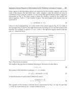
5.1 Initial Boundary Value Problem (IBVP)
Initial boundary value problem is formulated as per initial conditions and boundary
conditions. For the outer wall with uniform heat flux, heat conduction equation is written
with boundary conditions as (Dehra 2007d):
2
x
T
o
∂
∂
2
2
y
T
o
∂
∂
2
+
q
o

k
o
+ 0 in 0 x< t
o
< 0y< H<

(14)
Solar Energy Absorbers

121
x
T
o
∂
∂
⎛
⎜
⎝
⎞
⎟
⎠
−
α Sh
a
T
o
T
a
−
(

)
−
k
o
at x 0

(15)
x
T
o
∂
∂
h
o
T
o
T
f
−
(
)
hr T
o
T
i
−
(
)
+
k

o
at x t
o

(16)
For the inner wall with insulation, heat conduction equation with boundary conditions is:
2
x
T
i
∂
∂
2
2
y
T
i
∂
∂
2
+ 0 in L t
o
+ x< Lt
o
+ t
i
+< 0y< H<

(17)
x

T
i
∂
∂
h
s
T
i
T
s
−
(
)
k
i
0 at x L t
o
+ t
i
+

(18)
x
T
i
∂
∂
⎛
⎜
⎝

⎞
⎟
⎠
−
h
i
T
i
T
f
−
(
)
hr T
i
T
o
−
(
)
+
k
i
at x L t
o
+

(19)
Heat transport equation for air with its boundary value as:
θ y()

y
T
f
y()
∂
∂
⎡
⎢
⎣
⎤
⎥
⎦
T
f
y()+
T
o
y() T
i
y()+
2
⎡
⎢
⎣
⎤
⎥
⎦
− 0 in 0 y< H<

(20)

T
f
y() T
f
k() at y k
1
2
+
⎛
⎜
⎝
⎞
⎟
⎠
H
n
⋅ k0n1−()

(21)
In Eq. 21, k varies from 0 to (n-1), where n is number of nodes in y-ordinate. θ(y) =θ is
constant within the control volume at steady flow conditions, defined by following expression:
θ
v ρ Lc
p
h
c
W

(22)
5.2 Semi-analytical method

The partial differential equations are solved by applying initial conditions and lumped
parameter assumption to get the analytical solution. The temperatures of outer wall, inner
wall and air are obtained as:
T
o
h
a
T
a
h
o
T
f
+ hr T
i
+αS+
h
o
hr+ h
a
+
for
x
T
o
∂
∂
⎛
⎜
⎝

⎞
⎟
⎠
x0=
x
T
o
∂
∂
⎛
⎜
⎝
⎞
⎟
⎠
xt
o
=

(23)
T
i
h
s
T
s
⋅
h
i
T

f
⋅
+
h
r
T
o
⋅
+
h
i
hr+ h
s
+
for
x
T
i
∂
∂
⎛
⎜
⎝
⎞
⎟
⎠
xt
o
L+=
x

T
i
∂
∂
⎛
⎜
⎝
⎞
⎟
⎠
xt
o
L+ t
i
+=

(24)
Solar Collectors and Panels, Theory and Applications

122
T
f
T
o
T
i
+
2
T
f

k()⋅
T
o
T
i
+
2
−
⎡
⎢
⎣
⎤
⎥
⎦
e
2−
Δ
y
θ
⋅
⋅+

(25)
Where, ∆y=H/n is discretisation height of the control volume. Equation (6) is applicable
with in the control volume and it predicts particular solution for each ∆y from the values of
T
f
(k) at previous air node. The exponential solution of Equation (6) is semi-analytical in
nature because of its applicability for the nodes with in the physical domain of Fig. 1(b).
The numerical solutions are obtained by creation of additional heat exchange paths in the

computational grid. The additional heat exchange paths are created by incorporating
conduction heat flow along height of walls of thermosyphon and integrated radiation heat
exchange between composite surface nodes of outer and inner walls of thermosyphon
(Dehra, 2004). The numerical analysis involves (i) construction of nodal networks; (ii) energy
balance on the surface nodes located at solid-air edges of the walls; (iii) energy balance on
control volume for air passage; and (iv) computer solution of system of algebraic equations.
The energy balance equations for the N nodes involves formulation of (U
N,N
)-matrix with
conductance terms and heat source elements (Q
1,N
). Conductance terms describe entropy
flux over the discretised area (in W/K units) at the node. Inverse of U-matrix is multiplied
with heat source matrix to give temperature solution of the thermal network. In writing
nodal equations in matrix form, sign notation is adopted for automatic formulation of U-
matrix with unknown temperatures and heat source elements. Sum of all incoming heat
source elements and U-matrix conductance terms multiplied with temperature difference
with respect to the unknown temperatures at other nodes are equal to zero. The energy
balance is written in equation form for any general node (m,n) as per sign notation:
1
N
n
U
mn,
ΔT
mn,
×
()
∑
= 1

N
n
Q
mn,
∑
=
+ 0

(26)
Where U
m,n
is the conductance at node (m,n), ∆T
m,n
is the difference between unknown
temperature at the node (m,n) and unknown temperature at surrounding heat exchange
node. Q
N
is heat source term at the node (m,n). The detail of numerical method is provided in
(Dehra, 2004) and is omitted here by presenting its numerical solution procedure (Dehra, 2008a):
Step 1. Thermal properties are used to initialise the numerical solution. The conductance
values are calculated as per constitutive relations for conduction, convection,
radiation and heat transport.
Step 2. The corrected iterated value of the mass flow rate as depicted in Table 2 is obtained
from the numerical solution and is used for obtaining thermal capacity conductance
values.
Step 3. The heat transfer coefficients are calculated using temperatures obtained from the
analytical solution. The values of convective heat transfer coefficients obtained from
semi-analytical solution are also used in obtaining the numerical solution.
Step 4. The effect of integrated radiation heat exchange between surface nodes of outer and
inner wall is considered with radiosity-irradiation method assuming enclosure

analysis (Dehra, 2004). The radiation heat exchange factors are calculated for each
node using script factor matrix of size (20 X 20). Using radiation heat exchange factors
radiation conductance values are calculated, which also form matrix (20 X 20).
Solar Energy Absorbers

123
Step 5. Once conjugate heat exchange conductance values for 30 nodes are calculated, U-
matrix of size (30 X 30) is formulated. The U-matrix is formulated by obtaining off-
diagonal and diagonal entries as per constitutive relations and sign convention. The
inverse of U-matrix (30 X 30) is multiplied with heat source element matrix (1 X 30),
to obtain temperatures at 30 nodes (30 X 1) as per Equation (26).

18
19
20
21
22
23
24
25
26
27
28
29
0.15 0.45 0.75 1.05 1.35 1.65 1.95 2.25 2.55 2.85
Hei ght (m)
Temperature (
o
C)
Temperature of Outer Wall-Numerical Solution

Temperature of Outer Wall-Se mi-analytical Solution

(a)
6
8
10
12
14
16
18
20
22
24
0.15 0.45 0.75 1.05 1.35 1.65 1.95 2.25 2.55 2.85
Height (m)
Temperature (
o
C)
Te mperature of Inner Wall-Numerical Solution
Temperature of Inner Wall-Semi-analytical solution

(b)
-4
-2
0
2
4
6
8
10

12
14
16
18
20
0.15 0.45 0.75 1.05 1.35 1.65 1.95 2.25 2.55 2.85
Height (m)
Temperature (
o
C)
Temperature of Air-Numerical Solution
Temperature of Air-Se mi-analytical solution

(c)
Fig. 3. Comparison of temperature profiles from semi-analytical and numerical solutions
with height of solar thermosyphon for (a) outer wall; (b) inner wall; and (c) air
Solar Collectors and Panels, Theory and Applications

124
Figure 3 has compared the results obtained from traditional analytial model and numerical
model. A matrix solution procedure is adopted for solving energy balance nodal equations at
surface and air nodes. The improved numerical method has considered the effect of thermal
storage by incorporating conduction heat flow factors in y-direction for outer and inner walls
of thermosyphon. The heat conduction and radiation heat exchange between surface nodes
has improved the accuracy of a traditional analytical solution for predicting buoyancy-induced
mass flow rate through a solar thermosyphon. The conduction and convection conductance
terms are based on discretisation height ∆y, thermal capacity conductance (mc
p
) is based on
air-gap length ∆x, whilst integrated radiation conductance terms are based on both height ∆y

and width ∆x of the grid. The constitutive relations for obtaining conductance terms for
conductance (U’s) matrix are calculated over discretised control areas in y-z plane for
conduction heat flow, radiation and convection heat exchange. Whilst, heat transport
conductance terms are calculated from mass flow rate crossing the control volume in x-z plane
assuming no leakage or infiltration sources in the thermosyphon.
6. Photovoltaic duct wall
In an effort to enhance overall efficiency of PV module power generation system, a novel solar
energy utilization technique for co-generation of electric and thermal power is analyzed with a
photovoltaic duct wall system. A full scale experimental facility for a photovoltaic duct wall
was installed at Concordia University, Montréal, Concordia (Dehra, 2004). The photovoltaic
duct wall was comprised of a pair of glass coated PV modules, ventilated air passage and
polystyrene filled plywood board. In this case duct wall with air ventilation acts as cooling
channel for PV modules by reducing surface temperature of solar cells in PV modules and
slightly increases its efficiency for electric power generation. With air as fluid medium,
assessment of the potential use of photovoltaic duct wall to be used as a source of co-
generation of electric and thermal power can be performed by thermal analysis of material
properties of photovoltaic duct wall system (PV module, air and plywood board). The thermal
analysis of a photovoltaic duct wall has been performed through experimental and numerical
investigations. The measurement data collected from the experimental setup was for solar
intensities, currents, voltages, air velocities and temperatures of air and composite surfaces.
The measured temperatures were obtained as a function of height of photovoltaic duct wall.
The heat transfer rate from a photovoltaic duct wall is a measure of heat storage and thermal
storage capacities of its various components. The steady state heat transfer rate has been
predicted by performing two dimensional energy and mass balances on discretised section of
photovoltaic duct wall, to get solutions of one dimensional heat conduction and heat transport
equations. The assumptions of steady state heat transfer and lumped heat capacity are
validated by comparing heat losses along all major dimensions. The non-consideration of
transient analysis has been justified by comparing thermal losses along all major dimensions.
6.1 Experimental setup
The photovoltaic duct wall was installed on south facing façade of prefabricated outdoor

room. The outdoor room was setup at Concordia University, Montréal, Québec, Concordia
for conducting practical investigations (Dehra 2004, Dehra 2007a, Dehra 2009). The
photovoltaic duct wall was vertically inclined at 10° East of South on the horizontal plane.
The test section of photovoltaic duct wall was assembled in components with two
commercially available PV modules, air passage with air-gap width of 90 mm, plywood board
Solar Energy Absorbers

125
filled with polystyrene as insulation panel, side walls made up of Plexiglas and all parts
connected with wooden frames. The photovoltaic duct wall section was constructed with two
glass coated PV modules each of dimensions: (989 mm X 453 mm). The PV modules were
having glass coating of 3 mm attached on their exterior and interior sides. The plywood board
was assembled with 7 mm thick plywood board enclosure filled with 26 mm polystyrene. The
overall thickness of plywood board with polystyrene was 40 mm. The exterior dampers were
made of wood covered with an aluminium sheet. The heating, ventilating and air-conditioning
(HVAC) requirements were met in the outdoor room by a baseboard heater, an induced-draft
type exhaust fan and a split window air conditioner (Dehra, 2004). The heating was
supplemented by conditioning from the fresh air entering from the inlet damper through
photovoltaic duct wall. However, during the mild season of autumn for the duration of
conducting experimental runs, neither baseboard heater was used nor air-conditioning unit
was used for auxiliary heating or cooling inside the pre-fabricated outdoor room.

Air Inlet
Air Outlet
Air Velocity
Sensor
Damper D1
(Open)
Damper D3
(Closed)

Damper D2 (Open)
PV Module 2
Insulation Panel
PV Module 1
Thermocouples

Fig. 4. Schematic of the Experimental Setup
The pair of PV modules used for conducting experimental investigations was connected in
series for generation of electric power with a rheostat of maximum varying resistance up to 50
Ω. T-type thermocouples were used for obtaining thermal measurements from the test section
of photovoltaic module. As is illustrated in Fig. 4, three thermocouple sensors were placed at
the top, middle and bottom locations in the PV module, air-passage and insulation panel of
plywood board filled with polystyrene were used to measure local temperatures. Two
thermocouples were used to measure the inside test room air temperature and ambient air
temperature. The hybrid air ventilation created for the PV module test section was by natural
wind, or through buoyancy effect in the absence of wind (Dehra, 2004). The fan pressure was
used to achieve higher air velocities by operation of the exhaust fan fixed on opposite wall
with respect to wall of the test section (Dehra, 2004). The slight negative pressure was induced
for drawing low air velocities in absence of wind-induced pressure from the inlet damper into
the test section through the test room (Dehra, 2004). Air velocity sensor was placed
perpendicular to the walls of the PV module test section to record axial air velocities near its
outlet. The thermocouple outputs, currents, voltages, solar irradiation and air velocity signals
were connected to a data logger and a computer for data storage. The measurements collected
Solar Collectors and Panels, Theory and Applications

126
from the sensors were recorded as a function of air velocities or mass flow rate from the test
section with use of fan pressure. The experimental data from the data acquisition system was
collected and stored every two minutes in the computer (Dehra, 2004).
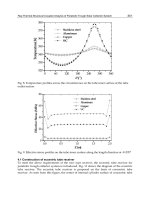
6.2 Temperature plots

The measurements collected from the sensors were recorded as a function of air velocities
through the PV module test section (Dehra, 2004): (i) Hybrid ventilation without use of fan
pressure; and (ii) Hybrid ventilation with use of fan pressure. The temperature measurements
were obtained from the PV module test section as a function of air velocities. The temperatures
were obtained for glass coated PV module, air passage and insulating panel in the wooden
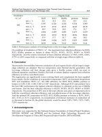
frame. The set of sample measurements obtained from outdoor experiments is presented in
Table 2. The temperature plots for PV module, insulating panel and air for different hybrid
ventilation conditions are illustrated in Figs. 5 and 6. The temperature plots are obtained
against the height of PV module test section for the data provided in Tables 2 to 4. The
variation of mean temperatures of PV module, insulating panel and air with approximately
steady solar noon irradiation with varying mass flow rates for the case of fan-induced hybrid
ventilation and buoyancy-induced hybrid ventilation are plotted in Figs. 7 to 9.


Run No.
S
(W m
-2
)
E
p

(W)
T
o

(° C)
T
s

(° C)
V
(m s
-1
)
Fan-induced hybrid ventilation
1 716.1 30.7 15.2 22.4 0.68
2 716.1 30.7 13.4 22.4 0.53
Buoyancy-induced hybrid ventilation
3 697.5 28.9 13.2 25.1 0.13
4 697.5 28.8 13.3 24.9 0.17
Run No.
T
p
(b)
(° C)
T
p
(m)
(° C)
T
p
(t)
(° C)
T
b
(b)
(° C)
T
b

(m)
(° C)
T
b
(t)
(° C)
T
a
(b)
(° C)
T
a
(m)
(° C)
T
a
(t)
(° C)
Fan-induced hybrid ventilation
1 35.4 33.8 36.8 20.6 24.7 29.1 18.8 21.7 19.4
2 35.9 34.6 37.9 20.9 25.0 29.5 19.3 22.5 19.9
Buoyancy-induced hybrid ventilation
3 40.8 44.9 46.8 27.9 34.8 38.0 21.3 29.5 29.8
4 39.9 45.0 46.8 28.4 35.0 38.3 21.7 28.3 29.8
Distance as per locations
shown in Fig. 4
T
p
(b)
(° C)

T
p
(m)
(° C)
T
p
(t)
(° C)
T
b
(b)
(° C)
T
b
(m)
(° C)
y (cm) 15 55 94 15 55
z (cm) 60 60 60 60 60
x (mm) 6.2 6.2 6.2 96.2 96.2
Distance as per locations
shown in Fig. 4
T
b
(t)
(° C)
T
a
(b)
(° C)
T

a
(m)
(° C)
T
a
(t)
(° C)
Air velocity
sensor
y (cm) 94 15 55 94 99
z (cm) 60 60 60 60 60
x (mm) 96.2 51.2 51.2 51.2 51.2
Note: x is horizontal; y is vertical; z is adjacent 3
rd
axis of x-y plane
Table 2. Outdoor measurements obtained from the experimental setup
Solar Energy Absorbers

127
Fan-induced hybrid ventilation
Run No. 2
32
33
34
35
36
37
38
39
40

0 0.2 0.4 0.6 0.8 1
Height of PV Module Test Section (m)
Temperature (
o
C)
PV Module Temperature

Fig. 5.(a) Temperature plot of PV module for fan-induced hybrid ventilation with height of
PV module test section
Fan-induced hybrid ventilation
Run No. 2
20
21
22
23
24
25
26
27
28
29
30
00.20.40.60.81
Height of PV Module Test Section (m)
Temperature (
o
C)
Insulating Panel Temperature

Fig. 5.(b) Temperature plot of insulating panel for fan-induced hybrid ventilation with

height of PV module test section
Fan-induced hybrid ventilation
Run No. 2
18
19
20
21
22
23
0 0.2 0.4 0.6 0.8 1
Height of PV Module Test Section (m)
Temperature (
o
C)
Air Temperature

Fig. 5.(c) Temperature plot of air for fan-induced hybrid ventilation with height of PV
module test section
Solar Collectors and Panels, Theory and Applications

128

Buoyancy-induced hybrid ventilation
Run No. 4
38
40
42
44
46
48

0 0.2 0.4 0.6 0.8 1
Height of PV Module Test Section (m)
Temperature (
o
C)
PV Module Temperature

Fig. 6.(a) Temperature plot of PV module for buoyancy-induced hybrid ventilation with
height of PV module test section
Buoyancy-induced hybrid ventilation
Run No. 4
27.5
29
30.5
32
33.5
35
36.5
38
39.5
0 0.2 0.4 0.6 0.8 1
Height of PV Module Test Section (m)
Temperature (
o
C)
Insulating Panel Temperature

Fig. 6.(b) Temperature plot of insulating panel for buoyancy-induced hybrid ventilation with
height of PV module test section
Buoyancy-induced hybrid air ventilation

Run No. 4
19
21
23
25
27
29
31
0 0.2 0.4 0.6 0.8 1
Height of PV Module Test Section (m)
Temperature (
o
C)
A
ir Temperature

Fig. 6.(c) Temperature plot of air for buoyancy-induced hybrid ventilation with height of PV
module test section
Solar Energy Absorbers

129
10
15
20
25
30
35
40
10:33:36 11:02:24 11:31:12 12:00:00 12:28:48
Time (Hrs.)

Temperature (
o
C)
704
708
712
716
720
724
Solar Irradiation
(Watts per sq.m.)
PV Module Temperature Insulating Panel Temperature
Air Temperature at Outlet Room Air Temperature
Outdoor Air Temperature Solar Irradiation

Fig. 7. Variation of mean temperatures of PV module, air and insulating panel with solar
irradiation under fan-induced hybrid ventilation
10
15
20
25
30
35
40
45
50
11:00:00 11:14:24 11:28:48 11:43:12 11:57:36 12:12:00 12:26:24
Time
Temperature (
o

C)
675
680
685
690
695
700
705
710
Solar Irradiation
(Watts per sq. m)
PV Module Temperature Outdoor Air Temperature
Insulating Panel Temperature Outlet Air Temperature
Room Air Temperature Solar Irradiation

Fig. 8.(a) Variation of mean temperatures of PV module, air and insulating panel with solar
irradiation under buoyancy-induced hybrid ventilation
0
2
4
6
8
10
12
10:58:00 11:12:24 11:26:48 11:41:12 11:55:36 12:10:00 12:24:24
Time (Hrs.)
Temp. Diff. (
o
C)
0

0.01
0.02
0.03
0.04
0.05
0.06
0.07
Mass Flow Rate
(kg/s)
PV Module Temperature Difference
Insulating Panel Temperature Difference
Air Temperature Difference
Mass Flow Rate

Fig. 8.(b) Temperature difference for PV module, insulating panel and air with height of PV
module test section for under fan-induced hybrid ventilation
Solar Collectors and Panels, Theory and Applications

130
0
2
4
6
8
10
12
14
16
11:00:00 11:14:24 11:28:48 11:43:12 11:57:36 12:12:00 12:26:24
Time

Temp. Diff. (
o
C)
0
0.005
0.01
0.015
0.02
0.025
0.03
Mass flow rate (kg/s)
PV Module Temperature Difference
Air Temperature Difference
Insulating Panel Temperature Difference
Massflow rate

Fig. 9. Temperature difference for PV module, insulating panel and air with height of PV
module test section under buoyancy-induced hybrid ventilation
6.3 Sensible heat storage capacity
The glass coated PV module test section with wooden frame was composed of non-
homogeneous materials having different densities, specific heats and thicknesses (2007 a).
The pair of glass coated PV module was having three layers of material viz., a flat sheet of
solar cells, with glass face sheets on its exterior and interior sides. The surface temperature
of PV module was assumed to be uniformly distributed in the three layers. The heat
capacity of the wooden frame and sealing material was having negligible effect on the
temperature of PV module, air or insulating panel because wood was used as construction
material and moreover the magnitude of the heat capacity of wood framing material was
not proportional to the face area of glass coated PV modules. Table 3 has presented sensible
heat capacities of glass coating, solar cells, air and polystyrene filled plywood board. For the
critical case of buoyancy-induced hybrid ventilation of Run no. 4 in Table 2, it was observed

that the difference of temperatures recorded by the top and bottom sensors for PV module,
air and insulating panel were 6.9 °C, 8.1 °C and 9.9 °C respectively. The temperature
differences were used for obtaining sensible heat storage capacities of various components
in y-ordinate. The heat storage capacities calculated were 59.6 kJ, 0.755 kJ and 510.7 kJ for

Component
ρ
n

(kg m
-3
)
C
n

(J Kg
-1
K
-1
)
d
n

(m)X10
-3
d
n
ρ
n
C

n

(J m
-2
K
-1
)
H
pv-T
(J K
-1
)
Glass coating 3000 500 3 4500 4171.5
PV module 2330 677 0.2 315.48 292.45
Glass coating 3000 500 3 4500 4171.5
Sub-total - - - - 8635.5
Air 1.1174 1000 90 100.56 93.22
Plywood 550 1750 7 6737.5 6245.66
Polystyrene 1050 1200 26 32760 30368.5
Plywood 550 1750 7 6737.5 6245.66
Sub-total - - - - 42953.0
Total - - - - 51588.5
Note: Heat capacities were calculated for face area of PV module test section of 0.927 m
2
.
Table 3. Sensible Heat Storage Capacities
Solar Energy Absorbers

131
PV module, air and insulating panel respectively. The values of heat capacities predicted

were negligible in comparison with the total daily solar irradiation on PV modules on the
day of conducting outdoor experiments. The values were estimated by assuming the
constant surface properties and ideal still air at the instance of collection of measurements.
Similar value of heat storage capacity in x-ordinate was obtained by assuming same
proportionate temperature difference along thicknesses in x-ordinate. It was found to be nil
in comparison with the value of heat capacity obtained for y-ordinate.
6.4 Thermal time constant
Thermal time constant is the time required for the outlet air temperature from the PV
module test section to attain 63.2 percent of the total difference in value attained in air
temperature following a step change in temperature of outdoor air crossing the inlet
opening (Dehra 2007 a). The data was selected observing a step change in the ambient air
temperature. The selected data was in steady state before and after the time-interval during
the unsteady state response of the outlet air temperature with the step change in ambient air
temperature. Thermal time constant under buoyancy-induced hybrid air ventilation was
estimated between 8-10 minutes in comparison to 2 minutes estimated under fan-induced
hybrid air ventilation. Therefore duration of time interval for obtaining measurements from
the data logger was selected for a minimum of two minutes to record any subtle
temperature changes. The graphs of outdoor and outlet air temperatures were plotted
against the time-interval of measured data for the cases of buoyancy and fan-induced hybrid
ventilation are illustrated in Fig. 10(a) and 10(b).
Thermal time constants of the PV module test section were function of ambient air
temperatures and air velocities and were therefore approximately calculated under
conditions of buoyancy-induced and fan-induced hybrid air ventilation.
6.5 Thermal storage capacity
Thermal storage capacities of various components of PV module test section are obtained
from their thermal conductivities. Time constant (T=ρ
d
C
pd
d

d
/h
d
) for each component is

12.3
11.7
10.2
38.1
36.2
34.7
10
10.5
11
11.5
12
12.5
13
13.5
14
10:01 10:03 10:05 10:07 10:09 10:11 10:13 10:15 10:17 10:19
Time
Outdoor Air Temperature (°C)
34
34.5
35
35.5
36
36.5
37

37.5
38
38.5
Outlet Air Temperature (°C)
Outdoor Air Temperature Outlet Air Temperature

Fig. 10.(a) Changes in outlet air temperature from PV module test section with a step change
in outdoor air temperature under buoyancy-induced hybrid ventilation
Solar Collectors and Panels, Theory and Applications

132
16.7
15.4
16.6
17.4
15.4
17.0
15.7
24.1
23.8
24.3
24.6
25.0
24.5
21.6
15
15.5
16
16.5
17

17.5
12:07 12:09 12:12 12:15 12:18
Time
Outdoor Air Temperature (°C)
18
19
20
21
22
23
24
25
26
Outlet Air Temperature (°C)
Outdoor Air Temperature Outlet Air Temperature

Fig. 10.(b) Changes in outlet air temperature from PV module test section with a step change
in outdoor air temperature under fan-induced hybrid ventilation
calculated in units of time from their heat capacities and film coefficients (Wm
-2
K
-1
).
Thermal storage capacity of PV module test section along its height is 15.9 KJ. Thermal
storage capacity in x-direction is negligible in comparison with the thermal storage capacity
in y-direction. Therefore temperature measurements were also felt necessary along the
height of PV module system to consider pattern of heat flow and heat transport. The
thermal storage capacities of components of PV module test section are presented in Table 4.

Component

k
d

(W m
-1
K
-1
)
d
n
ρ
n
C
n

(J m
-2
K
-1
)
H
d

(Wm
-2
K
-1
)
T
(sec)

PV module 0.91 9315.48 10 932
Air 0.02624 100.56 10.0 10
Plywood 0.0835 6737.5 10.0 674
Polystyrene 0.02821 32760 1.0 32760
Plywood 0.0835 6737.5 10.0 674
Component
ΔT
V

(K)
ΔT
H

(K)
Q
V

(KJ)
Q
H

(J)
PV module 6.9 0.04 5.8 0.2
Air 8.1 0.75 0.0 0.0
Plywood 9.9 0.40 0.55 0.16
Polystyrene 9.9 0.40 9.0 9.6
Plywood 9.9 0.40 0.55 0.16
Total - - 15.9 10.12
Table 4. Thermal Storage Capacities
Notes to the Table 4:

i) Equivalent thermal conductivity of glass coated PV module was calculated to be 0.91
Wm
-1
K
-1
; ii) temperature differences along y-direction i.e. along height of PV module test
section (0.993 m) were obtained from Table 2 for Run No. 4 in the case of buoyancy-induced
hybrid ventilation.
Solar Energy Absorbers

133
7. Conclusion
Solar energy absorbers use their selective properties for utilisation of solar energy. The
theory, analysis and methodology for selective design of solar energy absorbers is
presented. The radiation properties, sources of radiation, diffraction and measurement of
radiation are presented. The environmental health is discussed by presenting physiology of
solar radiation effects on the skin surface and mechanism of entropy generation by solar
energy absorbers. The supporting examples of solar thermosyphon and photovoltaic duct
wall are presented. The heat and body temperature control for human environmental health
is involved by presenting the physiology and metabolism of heat loss from the human body
surface. The modeling and experimental results for solar thermosyphon and photovoltaic
duct wall are elaborated for illustrating the cases of solar energy absorbers as solar collectors
and panels.
8. Acknowledgements
The Author (Guru of the Sikhs Dr. Himanshu Dehra) is a Doctor of Public Health Medicine
in Noise Behaviour. The sovereign King Guru Shri Shri Shri 1008 Dr. Himanshu Dehra
(Emperor of Earth, Wind, Sky and Lord of Moon) is grateful to his thirty two Queens for
their worships and allegiances for his everlasting Kingdom and is a capital industrialist of
enterprises:
I. Quality Tools & Measurement Systems (QTMS)

II. Quality Guard & Protection Systems (QGPS)
III. Quality Detection & Prevention Systems (QDPS)
IV. Quality Defence & Security Systems (QDSS)
V. Quality Arms & Ammunition Systems (QAAS)
VI. Gati Transportation Systems (GTS)
VII. Mati Logistics Systems (MLS)
VIII. Indrani Corporation (IC)
IX. Indrani Securities & Holdings (ISH)
X. Indrani Investments & Finances (IIF)
XI. Indrani Projects & Controls (IPC)
XII. Indrani Laws & Books (ILB)
XIII. Indrani Routes & Travels (IRT)
XIV. Indrani Herbs & Medicines (IHM)
XV. Indrani Designs & Furnishings (IDF)
XVI. Indrani Flags & Decorations (IFD)
XVII. Indrani Languages & Communications (ILC)
XVIII. Indrani Resources & Employees (IRE)
XIX. Indrani Commands & Forces (ICF)
XX. Indrani Events & Plans (IEP)
XXI. Indrani Agencies & Societies (IAS)
XXII. Indrani Religions & Worships (IRW)
XXIII. Indrani Forests & Timbers (IFT)
XXIV. Indrani Productions & Films (IPF)
XXV. Indrani Maps & Atlases (IMA)
XXVI. Indrani Reports & Presses (IRP)
Solar Collectors and Panels, Theory and Applications

134
XXVII. Indrani Crops & Animals (ICA)
XXVIII. Indrani Palaces & Monuments (IPM)

XXIX. Indrani Foods & Dairies (IFD)
XXX. Indrani Farms & Lands (IFL)
XXXI. Indrani Empires & States (IES)
XXXII. Indrani Marks & Trades (IMT)
9. References
Dehra, H. (2004). A Numerical and Experimental Study for Generation of Electric and
Thermal Power with Photovoltaic Modules Embedded in Building Façade,
submitted/unpublished Ph.D. thesis, Department of Building, Civil and
Environmental Engineering, Concordia University, Montréal, Québec, August
2004.
Dehra, H. (2006). A 1-D/2-D Model for an Exterior HVAC Rectangular Duct with a Steady
Solar Heat Flux Generation, orally presented at the proceedings of the Second
International Green Energy Conference, Oshawa, Ontario, June 25-29 2006, 1240-
1251, 0978123603.
Dehra, H. (2007a). The Effect of Heat and Thermal Storage Capacities of Photovoltaic Duct
Wall on Co-Generation of Electric and Thermal Power, in the proceedings of
American Institute of Chemical Engineers - AIChE 2007 Spring Meeting, Houston,
Texas, USA, April 22-26, 2007, Session 36a.
Dehra, H. (2007b). On Solar Building Energy Devices, 18th IASTED International Conference
on Modelling and Simulation, Montréal, Québec, May 30-June 1, 2007, 96-101,
9780889866645.
Dehra, H. (2007c). A Unified Theory for Stresses and Oscillations, Canadian Acoustics,
(September 2007), Vol. 35, 3, 132-133, 07116659.
Dehra, H. (2007d). Mathematical Analysis of a Solar Thermosyphon, International
conference on Advances in Energy Research, Department of Energy Science and
Engineering, Indian Institute of Technology, Bombay, December 2007, Macmillan,
USA, 023063432X.
Dehra, H. (2008a). The Entropy Matrix Generated Exergy Model for a Photovoltaic Heat
Exchanger under Critical Operating Conditions, International Journal of Exergy,
Vol. 5, Issue 2, 2008, 132-149, 17428297.

Dehra, H. (2008b). The Noise Scales and their Units, Canadian Acoustics, 36, 3, (September
2008) 78-79, 07116659.
Dehra, H. (2009). A Two Dimensional Thermal Network Model for a Photovoltaic Solar
Wall, Solar. Energy, Vol. 83, Issue 11, (November 2009) 1933-1942, 0038092X.
7
Space Power System –
Motivation, Review and Vision
Harijono Djojodihardjo
Aerospace Engineering Department
Faculty of Engineering, Universiti Putra Malaysia
43400 UPM SERDANG, Selangor, Malaysia
Department of Industrial Engineering
Faculty of Engineering, Universitas Al-Azhar Indonesia
Jalan Sisingamangaraja, Jakarta 121010, Indonesia
1. Introduction
The world’s population growth is exhausting the world’s limited supply of non-renewable
energy sources, and along with it, introducing significant anthropogenic environment and
climate change. Although the economic and business inertia trend to cling to the lure of non-
renewable energy resources, it is imperative that in the foreseeable future extensive
renewable or green energy sources should be progressively utilized to replace the non-
renewable ones and to sustain reasonable living standard for the entire world’s population.
The world’s dream of world’s socio-economic and technological equity and networking is
still far from being a reality, and many of the pioneering technology breakthrough for the
benefits of humanities, to some extend, contribute to their widening gap. Then it will be
timely and appropriate that a new vision for world’s “green” energy be shared by and
contributable to a fair distribution of world’s population, presently still grouped into
countries with unbalanced capacity distribution. In particular, judging from the large
population distribution and growth in developing countries compared to the developed
ones, the need and growth for energy resources will also be more or less similar.
Mankind success in space exploration has opened up their vision of the uniqueness of the

world we live in and the need for conserving our environment (Djojodihardjo, 2009;
Djojodihardjo & Varatharajoo, 2009), as illustrated in Figure 1. Such vision which has
inspired mankind to develop technological capabilities in atmospheric and space flight as
well as exploring new fromtiers beyond the earth’s atmosphere has been profoundly
articulated as far back as in 400 BC by Socrates in the well known verse: "Man must rise
above the Earth to the top of the atmosphere and beyond for only thus will he fully
understand the world in which he lives."
Mankind has acquired further wisdom and intelligence to observe, identify and respond to
the challenges posed by the observed global climate change from advances in space science,
technology and exploration, and its close relationship to sustainable life on earth and
mankind dramatically rising demand of energy. Such state of affairs is summarized in
Figure 1. With the appreciable climate change that has been observed and of great concern