Advanced Microwave and Millimeter Wave Technologies Devices, Circuits and Systems Part 13 pdf
Bạn đang xem bản rút gọn của tài liệu. Xem và tải ngay bản đầy đủ của tài liệu tại đây (1.57 MB, 40 trang )
AdvancedMicrowaveandMillimeterWave
Technologies:SemiconductorDevices,CircuitsandSystems472
2. Scalar and Vector Analyses of Bessel Beams (Yu & Dou, 2008a; Yu & Dou,
2008b)
2.1 Scalar analysis
In free space, the scalar field is governed by the following wave equation
2
2
2 2
1
( , ) ( , ) 0E r t E r t
c t
(1)
where
2
is the Laplacian operator, c is the velocity of light in free space, r
is the position
vector. Assuming that the angular frequency is
, the field ( , )E r t
can be written as
( , ) ( )exp( )E r t E r i t
(2)
Substituting (2) into (1), we have the homogeneous Helmholtz wave equation
2 2
( ) ( ) 0E r k E r
(3)
where
2
0 0
k
, is the wave number in free space. Applying the method of separation of
variables in cylindrical coordinates, we can derive the following solution from (3)
0
( , ) ( )exp( )exp( ( ))
n z
E r t E J k in i k z t
(4)
where
0
E
is a constant,
n
J
is the nth -order Bessel function of the first kind,
2 2
x
y
, cos
x
, siny
,
2 2 2
z
k k k
, k
and
z
k are the radial and longitudinal
wave numbers, respectively. Thus the time-average intensity of (4) can be given by
2
0
( , , 0) ( , , 0) | ( ) |
n
I z I z E J k
(5)
It can be seen from (5) that the intensity distribution always keeps unchanged in any plane
normal to the z-axis. This is the characteristic of the so-called nondiffracting Bessel beams.
When 0n , (4) represents the zero-order Bessel beams (i.e.
0
J
beams) presented by Durnin
in 1987 for the first time (Durnin, 1987). The central spot of a
0
J
beam is always bright, as
shown in Figs. 1(a) and 1(b). The size of the central spot is determined by
k
, and
when
k k
, it reaches the minimum possible diameter of about 3 4
, but when 0k
, (4)
reduces to a plane wave. The intensity profile of a
0
J
beam decays at a rate proportional
to
1
( )k
, so it is not square integrable (Durnin, 1987). However, its phase pattern is bright-
dark interphase concentric fringes, as shown in Fig. 1(c). An ideal Bessel beam extends
infinitely in the radial direction and contains infinite energy, and therefore a physically
generated Bessel beam is only an approximation to the ideal. Experimentally, the generation
of an approximate
0
J
beam is reported firstly by Durnin and co-workers (Durnin et al.,
1987). The geometrical estimate of the maximum propagation rang of a
0
J
beam is given by
2 1 2
max
[( ) 1]Z R k k
(6)
where
R
is the radius of the aperture in which the
0
J
beam is formed. We can see from (6)
that when R , then
max
Z , provided that k k
is a fixed value.
But for
0n , (4) denotes the high-order Bessel beams (i.e.
n
J
beams, n is an integer). The
intensity distribution of all the higher-order Bessel beams has zero on axis surrounded by
concentric rings. For example, when 3n , the
3
J
beam has a dark central spot and its first
bright ring appears at
4.201 k
, as illustrated in Figs. 2(a) and 2(b). However, the phase
pattern of the
n
J
beam is much different from that of the
0
J
beam. It has 2n arc sections
distributed evenly from the innermost to the outermost ring, as shown in Fig. 2(c).
(a) (b) (c)
Fig. 1. A
0
J
beam. (a) One-dimensional (1-D) intensity distribution. (b) 2-D intensity
distribution plotted in a gray-level representation. (c) Phase distribution (
0t
, 0z ). The
relevant parameters are incident wavelength of
3mm
, and aperture radius of 50
R
mm ,
1
0.962k mm
.
(a) (b) (c)
Fig. 2. A
3
J
beam. (a) 1-D intensity distribution. (b) 2-D intensity distribution. (c) Phase
distribution (
0t
, 0z
). The relevant parameters are the same as in Fig. 1,
except
1
0.638k mm
.
2.2 Vector analysis
2.2.1 TM and TE modes Bessel beams
In order to discover more characteristics of Bessel beams, the vector analyses should be
performed. By using the Hertzian vector potentials of electric and magnetic types
e
,
m
,
respectively, the fields are expressed as
2
e
e e e
E k
,
0 0
e
e
H i
(7)
0 0
m
m
E i
,
2
m
m m m
H k
(8)
where
e
and
m
are the solutions to vector Helmholtz wave equation. In a source-free
region, they satisfy the homogeneous vector Helmholtz equation, respectively. When the
choice of
e
e
z
and
m
m
z
, they are reduced to scalar Helmholtz equation
Pseudo-BesselBeamsinMillimeterandSub-millimeterRange 473
2. Scalar and Vector Analyses of Bessel Beams (Yu & Dou, 2008a; Yu & Dou,
2008b)
2.1 Scalar analysis
In free space, the scalar field is governed by the following wave equation
2
2
2 2
1
( , ) ( , ) 0E r t E r t
c t
(1)
where
2
is the Laplacian operator, c is the velocity of light in free space, r
is the position
vector. Assuming that the angular frequency is
, the field ( , )E r t
can be written as
( , ) ( )exp( )E r t E r i t
(2)
Substituting (2) into (1), we have the homogeneous Helmholtz wave equation
2 2
( ) ( ) 0E r k E r
(3)
where
2
0 0
k
, is the wave number in free space. Applying the method of separation of
variables in cylindrical coordinates, we can derive the following solution from (3)
0
( , ) ( )exp( )exp( ( ))
n z
E r t E J k in i k z t
(4)
where
0
E
is a constant,
n
J
is the nth -order Bessel function of the first kind,
2 2
x
y
, cos
x
, siny
,
2 2 2
z
k k k
, k
and
z
k are the radial and longitudinal
wave numbers, respectively. Thus the time-average intensity of (4) can be given by
2
0
( , , 0) ( , , 0) | ( ) |
n
I z I z E J k
(5)
It can be seen from (5) that the intensity distribution always keeps unchanged in any plane
normal to the z-axis. This is the characteristic of the so-called nondiffracting Bessel beams.
When 0n , (4) represents the zero-order Bessel beams (i.e.
0
J
beams) presented by Durnin
in 1987 for the first time (Durnin, 1987). The central spot of a
0
J
beam is always bright, as
shown in Figs. 1(a) and 1(b). The size of the central spot is determined by
k
, and
when
k k
, it reaches the minimum possible diameter of about 3 4
, but when 0k
, (4)
reduces to a plane wave. The intensity profile of a
0
J
beam decays at a rate proportional
to
1
( )k
, so it is not square integrable (Durnin, 1987). However, its phase pattern is bright-
dark interphase concentric fringes, as shown in Fig. 1(c). An ideal Bessel beam extends
infinitely in the radial direction and contains infinite energy, and therefore a physically
generated Bessel beam is only an approximation to the ideal. Experimentally, the generation
of an approximate
0
J
beam is reported firstly by Durnin and co-workers (Durnin et al.,
1987). The geometrical estimate of the maximum propagation rang of a
0
J
beam is given by
2 1 2
max
[( ) 1]Z R k k
(6)
where
R
is the radius of the aperture in which the
0
J
beam is formed. We can see from (6)
that when R , then
max
Z , provided that k k
is a fixed value.
But for
0n , (4) denotes the high-order Bessel beams (i.e.
n
J
beams, n is an integer). The
intensity distribution of all the higher-order Bessel beams has zero on axis surrounded by
concentric rings. For example, when 3n
, the
3
J
beam has a dark central spot and its first
bright ring appears at
4.201 k
, as illustrated in Figs. 2(a) and 2(b). However, the phase
pattern of the
n
J
beam is much different from that of the
0
J
beam. It has 2n arc sections
distributed evenly from the innermost to the outermost ring, as shown in Fig. 2(c).
(a) (b) (c)
Fig. 1. A
0
J
beam. (a) One-dimensional (1-D) intensity distribution. (b) 2-D intensity
distribution plotted in a gray-level representation. (c) Phase distribution (
0t
, 0z ). The
relevant parameters are incident wavelength of
3mm
, and aperture radius of 50
R
mm ,
1
0.962k mm
.
(a) (b) (c)
Fig. 2. A
3
J
beam. (a) 1-D intensity distribution. (b) 2-D intensity distribution. (c) Phase
distribution (
0t , 0z ). The relevant parameters are the same as in Fig. 1,
except
1
0.638k mm
.
2.2 Vector analysis
2.2.1 TM and TE modes Bessel beams
In order to discover more characteristics of Bessel beams, the vector analyses should be
performed. By using the Hertzian vector potentials of electric and magnetic types
e
,
m
,
respectively, the fields are expressed as
2
e
e e e
E k
,
0 0
e
e
H i
(7)
0 0
m
m
E i
,
2
m
m m m
H k
(8)
where
e
and
m
are the solutions to vector Helmholtz wave equation. In a source-free
region, they satisfy the homogeneous vector Helmholtz equation, respectively. When the
choice of
e
e
z
and
m
m
z
, they are reduced to scalar Helmholtz equation
AdvancedMicrowaveandMillimeterWave
Technologies:SemiconductorDevices,CircuitsandSystems474
2 2
0
e e
k ,
2 2
0
m m
k (9)
From (3) and (4), we have deduced that the
e
and
m
can take the form of
( )exp( )exp( ( ))
n z
J
k in i k z t
. Thus,
e
and
m
can be written in the form
( )exp( )exp[ ( )]
e
e e n z
z P J k in i k z t z
(10a)
( )exp( )exp[ ( )]
m
m m n z
z P J k in i k z t z
(10b)
where
e
P
and
m
P
are the electric and magnetic dipole moment, respectively. By substituting
(10) into (7) and (8) respectively, we finally obtain the TM and TE modes Bessel beams.
n
TM mode:
n
TE mode:
'
2
'
( )exp( )exp[ ( )]
( )exp( )exp[ ( )]
( )exp( )exp[ ( )]
( )exp( )exp[ ( )]
( )exp( )exp[ ( )]
e e z n z
e e z n z
ze e n z
e e n z
e e n z
E iP k k J k in i k z t
n
E Pk J k in i k z t
E P k J k in i k z t
n
H P J k in i k z t
H iP k J k in i k z t
H
0
ze
(11a)
'
'
2
( )exp( )exp[ ( )]
( )exp( )exp[ ( )]
0
( )exp( )exp[ ( )]
( )exp( )exp[ ( )]
( )exp( )exp[ (
m m n z
m m n z
zm
m m z n z
m m z n z
zm m n z
n
E P J k in i k z t
E iP k J k in i k z t
E
H iP k k J k in i k z t
n
H P k J k in i k z t
H P k J k in i k
)]z t
(11b)
From (11), their instant field vectors and intensity distributions for the TM or TE modes
Bessel beams can be easily obtained. Two examples for
0
TM and
0
TE modes Bessel beams are
illustrated in Figs. 3 and 4, respectively. From (11a), we can see that the transverse electric
field component of the
0
TM mode is only a radial part and thus it is radially polarized. This
can also be seen from Fig. 3(a). Similarly, the
0
TE mode is only an azimuthal component of
the electric field and thus is azimuthally polarized. Its field vectors at
0t are shown in Fig.
4(a).
2.2.2 Polarization States
To analyze the polarization states of Bessel beams, (11) in cylindrical coordinates are
transformed into rectangular coordinates. Applying the relationships:
cos sinx
,
and
sin cosy
, we have the following representations for the electric fields.
'
'
2
[ ( )cos ( )sin ]
exp( )exp[ ( )]
[ ( )sin ( )cos ]
exp( )exp[ ( )]
( )exp( )exp[ ( )]
xe n n
e z z
ye n n
e z z
ze e n z
n
E ik J k J k
Pk in i k z t
n
E ik J k J k
Pk in i k z t
E P k J k in i k z t
(12a)
'
'
[ ( ) cos ( )sin ]
exp( )exp[ ( )]
[ ( )sin ( )cos ]
exp( )exp[ ( )]
0
xm n n
m z
ym n n
m z
zm
n
E J k ik J k
P in i k z t
n
E J k ik J k
P in i k z t
E
(12b)
(a) (b)
(c) (d)
Fig. 3.
0
TM mode Bessel beam. (a) Instant vector diagram for the transverse component of
the electric field (
0t
, 0z
). (b) The transverse electric field intensity (
2 2
| | | |
e e
I E E
).
(c) The longitudinal electric field intensity (
2
| |
z ze
I E ) and (d) the total electric filed intensity
(
z
I I I
). The color bars illustrate the relative intensity. The relevant parameters
are
3mm
,
1
2.004k mm
,
1
0.608
z
k mm
, and 10
R
mm
.
Pseudo-BesselBeamsinMillimeterandSub-millimeterRange 475
2 2
0
e e
k
,
2 2
0
m m
k (9)
From (3) and (4), we have deduced that the
e
and
m
can take the form of
( )exp( )exp( ( ))
n z
J
k in i k z t
. Thus,
e
and
m
can be written in the form
( )exp( )exp[ ( )]
e
e e n z
z P J k in i k z t z
(10a)
( )exp( )exp[ ( )]
m
m m n z
z P J k in i k z t z
(10b)
where
e
P
and
m
P
are the electric and magnetic dipole moment, respectively. By substituting
(10) into (7) and (8) respectively, we finally obtain the TM and TE modes Bessel beams.
n
TM mode:
n
TE mode:
'
2
'
( )exp( )exp[ ( )]
( )exp( )exp[ ( )]
( )exp( )exp[ ( )]
( )exp( )exp[ ( )]
( )exp( )exp[ ( )]
e e z n z
e e z n z
ze e n z
e e n z
e e n z
E iP k k J k in i k z t
n
E Pk J k in i k z t
E P k J k in i k z t
n
H P J k in i k z t
H iP k J k in i k z t
H
0
ze
(11a)
'
'
2
( )exp( )exp[ ( )]
( )exp( )exp[ ( )]
0
( )exp( )exp[ ( )]
( )exp( )exp[ ( )]
( )exp( )exp[ (
m m n z
m m n z
zm
m m z n z
m m z n z
zm m n z
n
E P J k in i k z t
E iP k J k in i k z t
E
H iP k k J k in i k z t
n
H P k J k in i k z t
H P k J k in i k
)]z t
(11b)
From (11), their instant field vectors and intensity distributions for the TM or TE modes
Bessel beams can be easily obtained. Two examples for
0
TM and
0
TE modes Bessel beams are
illustrated in Figs. 3 and 4, respectively. From (11a), we can see that the transverse electric
field component of the
0
TM mode is only a radial part and thus it is radially polarized. This
can also be seen from Fig. 3(a). Similarly, the
0
TE mode is only an azimuthal component of
the electric field and thus is azimuthally polarized. Its field vectors at
0t
are shown in Fig.
4(a).
2.2.2 Polarization States
To analyze the polarization states of Bessel beams, (11) in cylindrical coordinates are
transformed into rectangular coordinates. Applying the relationships:
cos sinx
,
and
sin cosy
, we have the following representations for the electric fields.
'
'
2
[ ( )cos ( )sin ]
exp( )exp[ ( )]
[ ( )sin ( )cos ]
exp( )exp[ ( )]
( )exp( )exp[ ( )]
xe n n
e z z
ye n n
e z z
ze e n z
n
E ik J k J k
Pk in i k z t
n
E ik J k J k
Pk in i k z t
E P k J k in i k z t
(12a)
'
'
[ ( ) cos ( )sin ]
exp( )exp[ ( )]
[ ( )sin ( )cos ]
exp( )exp[ ( )]
0
xm n n
m z
ym n n
m z
zm
n
E J k ik J k
P in i k z t
n
E J k ik J k
P in i k z t
E
(12b)
(a) (b)
(c) (d)
Fig. 3.
0
TM mode Bessel beam. (a) Instant vector diagram for the transverse component of
the electric field (
0t , 0z ). (b) The transverse electric field intensity (
2 2
| | | |
e e
I E E
).
(c) The longitudinal electric field intensity (
2
| |
z ze
I E ) and (d) the total electric filed intensity
(
z
I I I
). The color bars illustrate the relative intensity. The relevant parameters
are
3mm
,
1
2.004k mm
,
1
0.608
z
k mm
, and 10
R
mm
.
AdvancedMicrowaveandMillimeterWave
Technologies:SemiconductorDevices,CircuitsandSystems476
(a) (b)
Fig. 4.
0
TE
mode Bessel beam. (a) Instant vector diagram for the transverse component of the
electric field (
0t , 0z ). (b) The transverse electric field intensity. The relevant parameters
are the same as in Fig. 3, except
1
1.503k mm
, and
1
1.459
z
k mm
.
The total electric fields of
x
E
and
y
E are given by, respectively
1 2
x
xe xm
E
A E A E ,
1 2y ye ym
E A E A E (13)
where
1
A
and
2
A
are the proportional coefficients. Let 1
e
P , then
m
P i
. Substituting
(12) into (13), we can deduce the following representations:
1
exp( )exp( )exp[ ( )]
x xA z
E E i in i k z t
,
2
exp( )exp( )exp[ ( )]
y yA z
E E i in i k z t
(14)
where
2 2
1 2
( sin ) ( cos )
xA
E B B
,
2 2
1 2
( cos ) ( sin )
yA
E B B
,
'
1
1 2
( ) ( )
z
n n
A nk
B J k A kk J k
,
'
2 1 2
( ) ( )
z n n
nk
B Ak k J k A J k
,
2
1
1
cos
arctan( )
sin
B
B
,
2
2
1
sin
arctan( )
cos
B
B
.
The polarization states of Bessel beams are discussed as follows:
Case 1)
2 1
K
, where 0,1,2 K is an integer. The Bessel beam is linearly polarized.
To satisfy this case and assume that 0n , it is demanded from (14) that
1
0A and
2
0A ,
or
1
0A and
2
0A . Under these conditions, we can acquire the zero-order Bessel beam with
linear polarization, as shown schematically in Figs. 5 and 6.
Case 2)
2 1
2
and
x
A yA
E E . The Bessel beam is left-hand circularly polarized. To
satisfy these requirements, the demand of
1 2
z
A
A k k can be derived from (14). The left-
hand circularly polarized Bessel beam is illustrated in Fig. 7.
Case 3)
2 1
2
and
x
A yA
E E . The Bessel beam become right-hand circularly
polarized. Similarly, the demand of
1 2
z
A
A k k is needed. Fig. 8 shows the right-hand
circularly polarized Bessel beam.
Case 4) In other cases, the Bessel beam is elliptically polarized.
(a) (b) (c)
Fig. 5. Linearly polarized Bessel beam. (a)-(c) Vector diagrams of the transverse component
of the electric field at three different instants:
t 0
, t 0.5T
, t T
,
2T
, respectively.
The parameters used in Fig. 5 are 0.25k k
, 0n ,
1
0A
, and
2
0A
.
(a) (b) (c)
Fig. 6. Linearly polarized Bessel beam. (a)-(c) Vector diagrams of the transverse component
of the electric field at three different instants: t 0
, t 0.5T
, t T
, respectively. The
parameters used in Fig. 6 are the same as in Fig. 5, except
1
0A
, and
2
0A
.
(a) (b) (c)
Fig. 7. Left-hand circularly polarized Bessel beam. (a)-(c) Vector diagrams of the transverse
component of the electric field at three different instants:
t 0
, t 0.125T
, t 0.25T ,
respectively. The relevant parameters are
0.4k k
, and
1 2
z
A
A k k .
Pseudo-BesselBeamsinMillimeterandSub-millimeterRange 477
(a) (b)
Fig. 4.
0
TE
mode Bessel beam. (a) Instant vector diagram for the transverse component of the
electric field (
0t , 0z
). (b) The transverse electric field intensity. The relevant parameters
are the same as in Fig. 3, except
1
1.503k mm
, and
1
1.459
z
k mm
.
The total electric fields of
x
E
and
y
E are given by, respectively
1 2
x
xe xm
E
A E A E ,
1 2y ye ym
E A E A E
(13)
where
1
A
and
2
A
are the proportional coefficients. Let 1
e
P
, then
m
P i
. Substituting
(12) into (13), we can deduce the following representations:
1
exp( )exp( )exp[ ( )]
x xA z
E E i in i k z t
,
2
exp( )exp( )exp[ ( )]
y yA z
E E i in i k z t
(14)
where
2 2
1 2
( sin ) ( cos )
xA
E B B
,
2 2
1 2
( cos ) ( sin )
yA
E B B
,
'
1
1 2
( ) ( )
z
n n
A nk
B J k A kk J k
,
'
2 1 2
( ) ( )
z n n
nk
B Ak k J k A J k
,
2
1
1
cos
arctan( )
sin
B
B
,
2
2
1
sin
arctan( )
cos
B
B
.
The polarization states of Bessel beams are discussed as follows:
Case 1)
2 1
K
, where 0,1,2 K
is an integer. The Bessel beam is linearly polarized.
To satisfy this case and assume that 0n
, it is demanded from (14) that
1
0A
and
2
0A ,
or
1
0A and
2
0A . Under these conditions, we can acquire the zero-order Bessel beam with
linear polarization, as shown schematically in Figs. 5 and 6.
Case 2)
2 1
2
and
x
A yA
E E
. The Bessel beam is left-hand circularly polarized. To
satisfy these requirements, the demand of
1 2
z
A
A k k
can be derived from (14). The left-
hand circularly polarized Bessel beam is illustrated in Fig. 7.
Case 3)
2 1
2
and
x
A yA
E E
. The Bessel beam become right-hand circularly
polarized. Similarly, the demand of
1 2
z
A
A k k
is needed. Fig. 8 shows the right-hand
circularly polarized Bessel beam.
Case 4) In other cases, the Bessel beam is elliptically polarized.
(a) (b) (c)
Fig. 5. Linearly polarized Bessel beam. (a)-(c) Vector diagrams of the transverse component
of the electric field at three different instants: t 0 , t 0.5T , t T ,
2T
, respectively.
The parameters used in Fig. 5 are 0.25k k
, 0n ,
1
0A , and
2
0A .
(a) (b) (c)
Fig. 6. Linearly polarized Bessel beam. (a)-(c) Vector diagrams of the transverse component
of the electric field at three different instants:
t 0 , t 0.5T , t T , respectively. The
parameters used in Fig. 6 are the same as in Fig. 5, except
1
0A , and
2
0A .
(a) (b) (c)
Fig. 7. Left-hand circularly polarized Bessel beam. (a)-(c) Vector diagrams of the transverse
component of the electric field at three different instants:
t 0 , t 0.125T , t 0.25T ,
respectively. The relevant parameters are
0.4k k
, and
1 2
z
A
A k k .
AdvancedMicrowaveandMillimeterWave
Technologies:SemiconductorDevices,CircuitsandSystems478
(a) (b) (c)
Fig. 8. Right-hand circularly polarized Bessel beam. (a)-(c) Vector diagrams of the transverse
component of the electric field at three different instants:
t 0 , t 0.125T , t 0.25T ,
respectively. The relevant parameters are
0.4k k
, and
1 2
z
A
A k k .
2.2.3 Energy Density and Poynting Vector
Using the above equations (11), the total time-average electromagnetic energy density for
the transverse modes, TE or TM, is calculated to be
2 2 2 2 2 2 ' 2
1 1 1
| | | | {( ) ( )[( ) ( ) ]}
4 4 4
n
n z n
nJ
w E H k J k k k J
(15)
And the time-average Poynting vector power density is given by
*
2 ' 2 2
1
Re( ) [( ) ( ) ] ( )
2
n
z n n
nJ n
S E H k k J z k J
(16)
From (15) or (16), it can immediately be seen that neither
w nor S
depends on the
propagation distance
z
. This means the time-average energy density does not change along
the
z axis, and our solutions clearly represent nondiffracting Bessel beams. In addition, from
(16), we note that
S
has the longitudinal and transverse components, which determine the
flow of energy along the
z
axis and perpendicular to the z-axis, respectively. However, when
n=0, corresponding to
0
TM or
0
TE mode,
S
is directed strictly along the z-axis and is
proportional to
2
1
J
.
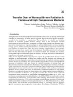
3. Generation of pseudo-Bessel Beams by BOEs (Yu & Dou, 2008c; Yu & Dou,
2008d)
In optics, lots of methods for creating pseudo-Bessel Beams have been suggensted, such as
narrow annular slit (Durnin et al., 1987), computer-generated holograms (CGHs) (Turunen
et al., 1988), Fabry-Perot cavity (Cox & Dibble, 1992), axicon (Scott & McArdle, 1992), optical
refracting systems (Thewes et al., 1991), diffractive phase elements (DPEs) (Cong et al., 1998)
and so on. However, at millimeter and sub-millimeter wavebands, only two methods of
production Bessel beams have been proposed currently, i.e., axicon (Monk et al., 1999) and
computer-generated amplitude holograms (Salo et al., 2001; Meltaus et al., 2003). Although
the method of using axicon is very simple, only a zero-order Bessel beam can be generated.
The other method relying on holograms can produce various types of diffraction-free beams,
but their diffraction efficiencies are only around 45% (Arlt & Dholakia, 2000) owing to using
amplitude holograms. In order to overcome these limitations mentioned above, in our work,
binary optical elements (BOEs) are employed and designed for producing pseudo-Bessel
Beams in millimeter and sub-millimeter range for the first time. The suitable design tool is to
combine a genetic algorithm (GA) for global optimization with a two-dimensional finite-
difference time-domain (2-D FDTD) method for rigours eletromagnetic computation.
3.1 Description of the design tool
3.1.1 FDTD method computational model
The electric field distribution of the
nth -order Bessel beam in the cylindrical coordinates
system is rewritten as:
0
( , , ) ( ) exp( )exp( )
n z
E
z E J k in ik z
(17)
All Bessel beams are circularly symmetric, thus our calculations are concerned only with
radically symmetric system. The feature sizes of BOEs are on the order of or less than a
millimeter wavelength, the methods of full wave analysis are needed to calculate the
diffractive fields of BOEs. The 2-D FDTD method (Yee, 1966) is employed to compute the
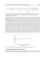
field diffracted by the BOE in our work. The Computational model of the FDTD method is
shown schematically in Fig. 9, in which the BOE is used to convert an incident Gaussian-
profile beam on the input plane into a Bessel-profile beam on the output plane.
1
z is the
distance between the input plane and the BOE, and
2
z is the distance between the BOE and
the output plane; the aperture radius of the BOE, which is represented by
R
, is the same as
that of the input and output planes;
1
n and
2
n represent the refractive indices of the free space
and the BOE, respectively; and
z is the symmetric axis and the magnetic wall is set on it to
save the required memory and computing time.
When a Gaussian beam is normally incident from the input plane onto the left side of the
BOE, its wave front is modulated by the BOE, and a desired Bessel beam is obtained on the
output plane. It is worthy to point out that our design goal is to acquire a desired Bessel
beam in the near field (i.e. the output plane). If one wants to obtain a desired field in the far
field, an additional method, like angular-spectrum propagation method (Feng et al.,2003),
should be employed to determine the far field.
Fig. 9. Schematic diagram of 2-D FDTD computational model
3.1.2 Genetic Algorithm (GA)
To fabricate conveniently in technics, the DOE, with circular symmetry and aperture
radius
R
, should be divided into concentric rings with identical width
but different
Pseudo-BesselBeamsinMillimeterandSub-millimeterRange 479
(a) (b) (c)
Fig. 8. Right-hand circularly polarized Bessel beam. (a)-(c) Vector diagrams of the transverse
component of the electric field at three different instants:
t 0
, t 0.125T
, t 0.25T ,
respectively. The relevant parameters are
0.4k k
, and
1 2
z
A
A k k
.
2.2.3 Energy Density and Poynting Vector
Using the above equations (11), the total time-average electromagnetic energy density for
the transverse modes, TE or TM, is calculated to be
2 2 2 2 2 2 ' 2
1 1 1
| | | | {( ) ( )[( ) ( ) ]}
4 4 4
n
n z n
nJ
w E H k J k k k J
(15)
And the time-average Poynting vector power density is given by
*
2 ' 2 2
1
Re( ) [( ) ( ) ] ( )
2
n
z n n
nJ n
S E H k k J z k J
(16)
From (15) or (16), it can immediately be seen that neither
w nor S
depends on the
propagation distance
z
. This means the time-average energy density does not change along
the
z axis, and our solutions clearly represent nondiffracting Bessel beams. In addition, from
(16), we note that
S
has the longitudinal and transverse components, which determine the
flow of energy along the
z
axis and perpendicular to the z-axis, respectively. However, when
n=0, corresponding to
0
TM or
0
TE mode,
S
is directed strictly along the z-axis and is
proportional to
2
1
J
.
3. Generation of pseudo-Bessel Beams by BOEs (Yu & Dou, 2008c; Yu & Dou,
2008d)
In optics, lots of methods for creating pseudo-Bessel Beams have been suggensted, such as
narrow annular slit (Durnin et al., 1987), computer-generated holograms (CGHs) (Turunen
et al., 1988), Fabry-Perot cavity (Cox & Dibble, 1992), axicon (Scott & McArdle, 1992), optical
refracting systems (Thewes et al., 1991), diffractive phase elements (DPEs) (Cong et al., 1998)
and so on. However, at millimeter and sub-millimeter wavebands, only two methods of
production Bessel beams have been proposed currently, i.e., axicon (Monk et al., 1999) and
computer-generated amplitude holograms (Salo et al., 2001; Meltaus et al., 2003). Although
the method of using axicon is very simple, only a zero-order Bessel beam can be generated.
The other method relying on holograms can produce various types of diffraction-free beams,
but their diffraction efficiencies are only around 45% (Arlt & Dholakia, 2000) owing to using
amplitude holograms. In order to overcome these limitations mentioned above, in our work,
binary optical elements (BOEs) are employed and designed for producing pseudo-Bessel
Beams in millimeter and sub-millimeter range for the first time. The suitable design tool is to
combine a genetic algorithm (GA) for global optimization with a two-dimensional finite-
difference time-domain (2-D FDTD) method for rigours eletromagnetic computation.
3.1 Description of the design tool
3.1.1 FDTD method computational model
The electric field distribution of the
nth -order Bessel beam in the cylindrical coordinates
system is rewritten as:
0
( , , ) ( ) exp( )exp( )
n z
E
z E J k in ik z
(17)
All Bessel beams are circularly symmetric, thus our calculations are concerned only with
radically symmetric system. The feature sizes of BOEs are on the order of or less than a
millimeter wavelength, the methods of full wave analysis are needed to calculate the
diffractive fields of BOEs. The 2-D FDTD method (Yee, 1966) is employed to compute the
field diffracted by the BOE in our work. The Computational model of the FDTD method is
shown schematically in Fig. 9, in which the BOE is used to convert an incident Gaussian-
profile beam on the input plane into a Bessel-profile beam on the output plane.
1
z is the
distance between the input plane and the BOE, and
2
z is the distance between the BOE and
the output plane; the aperture radius of the BOE, which is represented by
R
, is the same as
that of the input and output planes;
1
n and
2
n represent the refractive indices of the free space
and the BOE, respectively; and
z is the symmetric axis and the magnetic wall is set on it to
save the required memory and computing time.
When a Gaussian beam is normally incident from the input plane onto the left side of the
BOE, its wave front is modulated by the BOE, and a desired Bessel beam is obtained on the
output plane. It is worthy to point out that our design goal is to acquire a desired Bessel
beam in the near field (i.e. the output plane). If one wants to obtain a desired field in the far
field, an additional method, like angular-spectrum propagation method (Feng et al.,2003),
should be employed to determine the far field.
Fig. 9. Schematic diagram of 2-D FDTD computational model
3.1.2 Genetic Algorithm (GA)
To fabricate conveniently in technics, the DOE, with circular symmetry and aperture
radius
R
, should be divided into concentric rings with identical width
but different
AdvancedMicrowaveandMillimeterWave
Technologies:SemiconductorDevices,CircuitsandSystems480
depth
x
, as shown in Fig. 10. The width
equals
R
K ,
K
is a prescribed positive integer.
The maximal depth of a ring is
max 2
( 1)x n
, in which
2
n
is the refractive index of the
BOE. In BOEs design, the depth
x
of each ring can take only a discrete value. Provided that
the maximal depth of a ring is quantified into
M
-level, in general case, 2
a
M
, where
a
is a
integer, the minimal depth of a ring is
max
x
x M . Therefore, the depth
x
of each ring can
take only one of the values in the set of
,2 , ,
x
x M x . Thus, the different combination of
the depth
x
of each ring, i.e.,
1
K
k
k
X
x
, where
,2 , ,
k
x
x x M x , represents the
different BOE profile. To obtain the BOE profile which satisfies the design requirement,the
different combination
X
should be calculated, and the optimum combination is gained
finally. In fact, this is a combinatorial optimization problem (COP). The GA (Haupt, 1995;
Weile & Michielssen, 1997) is adopted for optimizing the BOE profile. It operates on the
chromosome, each of which is composed of genes associated with a parameter to be
optimized. For instance, in our case, a chromosome corresponds to a set
X
which describes
the BOE profile, and a gene corresponds to the depth
x
of a ring.
The first step of the GA is to generate an initial population, whose chromosomes are made
by random selection of discrete values for the genes. Next, a fitness function, which
describes the different between the desired field
d
E and the calculated field
c
E obtained by
using 2-D FDTD method, will be evaluated for each chromosome. In our study, the fitness
function is simply defined as:
2
1
(| | | |)
U
c d
u u
u
fitness E E
(18)
in which
c
u
E and
d
u
E are the calculated field and the desired field at the uth sample ring of the
output plane, respectively. Then, based on the fitness of each chromosome, the next
generation is created by the reproduction process involved crossover, mutation, and
selection. Last, the GA process is terminated after a prespecified number of
generations
max
Gen . The flow chart of the GA procedure is shown in Fig. 11.
Fig. 10. Division of the BOE profile into the rings with identical width
but different
depths
x
Fig. 11. The flow chart of the GA procedure
3.2 Numerical simulation results
In order to evaluate the quality of the designed BOE, we introduce the efficiency
and the
root mean square (
R
MS ) describing the BOE profile error (Feng et al.,2003), which are
defined as, respectively.
2
1
2
1
| |
| |
U
c c
u u
u
V
i i
v v
v
E S
E S
(19)
1 2
2 2 2
1
1
(| | | | )
1
U
c d
u u
u
RMS E E
U
(20)
where
i
v
S and
c
u
S are the areas of the vth and uth sample ring of the input and output planes,
respectively;
i
v
E is the incident field at the vth sample ring of the input plane, and
c
u
E and
d
u
E are the calculated field and the desired field at theuth sample ring of the output
plane. To demonstrate the utility of the design method, we present three examples herein in
which an incident Gaussian beam is converted into a zero-order, a first order and a second
order Bessel beam respectively. The same parameters in three examples are as follows: an
incident Gaussian beam waist of
0
4w
1
1.0n
,
2
1.45n
,
1
2z
,
2
6z
,
18
, 8R
, 144
K
, 8M
,U V K
. From three cases, it is clearly seen that the
fields diffracted by the designed BOE’s on the output plane agree well with the desired
electric field intensity distributions.
Pseudo-BesselBeamsinMillimeterandSub-millimeterRange 481
depth
x
, as shown in Fig. 10. The width
equals
R
K ,
K
is a prescribed positive integer.
The maximal depth of a ring is
max 2
( 1)x n
, in which
2
n
is the refractive index of the
BOE. In BOEs design, the depth
x
of each ring can take only a discrete value. Provided that
the maximal depth of a ring is quantified into
M
-level, in general case, 2
a
M
, where
a
is a
integer, the minimal depth of a ring is
max
x
x M . Therefore, the depth
x
of each ring can
take only one of the values in the set of
,2 , ,
x
x M x
. Thus, the different combination of
the depth
x
of each ring, i.e.,
1
K
k
k
X
x
, where
,2 , ,
k
x
x x M x
, represents the
different BOE profile. To obtain the BOE profile which satisfies the design requirement,the
different combination
X
should be calculated, and the optimum combination is gained
finally. In fact, this is a combinatorial optimization problem (COP). The GA (Haupt, 1995;
Weile & Michielssen, 1997) is adopted for optimizing the BOE profile. It operates on the
chromosome, each of which is composed of genes associated with a parameter to be
optimized. For instance, in our case, a chromosome corresponds to a set
X
which describes
the BOE profile, and a gene corresponds to the depth
x
of a ring.
The first step of the GA is to generate an initial population, whose chromosomes are made
by random selection of discrete values for the genes. Next, a fitness function, which
describes the different between the desired field
d
E and the calculated field
c
E obtained by
using 2-D FDTD method, will be evaluated for each chromosome. In our study, the fitness
function is simply defined as:
2
1
(| | | |)
U
c d
u u
u
fitness E E
(18)
in which
c
u
E and
d
u
E are the calculated field and the desired field at the uth sample ring of the
output plane, respectively. Then, based on the fitness of each chromosome, the next
generation is created by the reproduction process involved crossover, mutation, and
selection. Last, the GA process is terminated after a prespecified number of
generations
max
Gen . The flow chart of the GA procedure is shown in Fig. 11.
Fig. 10. Division of the BOE profile into the rings with identical width
but different
depths
x
Fig. 11. The flow chart of the GA procedure
3.2 Numerical simulation results
In order to evaluate the quality of the designed BOE, we introduce the efficiency
and the
root mean square (
R
MS ) describing the BOE profile error (Feng et al.,2003), which are
defined as, respectively.
2
1
2
1
| |
| |
U
c c
u u
u
V
i i
v v
v
E S
E S
(19)
1 2
2 2 2
1
1
(| | | | )
1
U
c d
u u
u
RMS E E
U
(20)
where
i
v
S and
c
u
S are the areas of the vth and uth sample ring of the input and output planes,
respectively;
i
v
E is the incident field at the vth sample ring of the input plane, and
c
u
E and
d
u
E are the calculated field and the desired field at theuth sample ring of the output
plane. To demonstrate the utility of the design method, we present three examples herein in
which an incident Gaussian beam is converted into a zero-order, a first order and a second
order Bessel beam respectively. The same parameters in three examples are as follows: an
incident Gaussian beam waist of
0
4w
1
1.0n
,
2
1.45n
,
1
2z
,
2
6z
,
18
, 8R
, 144
K
, 8M ,U V K . From three cases, it is clearly seen that the
fields diffracted by the designed BOE’s on the output plane agree well with the desired
electric field intensity distributions.
AdvancedMicrowaveandMillimeterWave
Technologies:SemiconductorDevices,CircuitsandSystems482
(a) (b)
Pseudo-BesselBeamsinMillimeterandSub-millimeterRange 483
(a) (b)
(c) (d)
Fig. 12. Generation of a
0
J
beam on the output plane. 3mm
,
1
0.7635k mm
,
94.494%
and 5.562%RMS . (a) Part of the optimized BOE profile. (b) The desired and the designed
transverse intensity distribution on the output plane. (c) The 2-D transverse intensity
distribution plotted in a gray-level representation, and (d) the 3-D transverse intensity
distribution.
(a) (b)
(c) (d)
Fig. 13. Production of a
1
J
beam on the output plane. 3mm
,
1
0.6911k mm
, 96.283%
and 2.806%RMS . (a) Part of the optimized BOE profile. (b) The desired and the designed
transverse intensity distribution on the output plane. (c) The 2-D transverse intensity
distribution, and (d) the 3-D transverse intensity distribution.
(a) (b)
(c) (d)
Fig. 14. Creation of a
2
J
Bessel beam on the output plane. 0.333mm
,
1
5.6406k mm
,
97.263%
and 1.845%RMS . (a) Part of the optimized BOE profile. (b) The desired and
the designed transverse intensity distribution on the output plane. (c) The 2-D transverse
intensity distribution, and (d) the 3-D transverse intensity distribution.
4. Production of approximate Bessel beams using binary axicons (Yu & Dou,
2009)
Currently, numerous ways for generating pseudo-Bessel beams have been proposed, among
which using axicon is the most popular method, owing to its simplicity of configuration and
easy realization. However, at millemter and sub-millimter wavebands, classical cone axicons
are usually bulk ones and therefore have many disadvantages, like heavy weight, large
volume and thus increased absorption loss in the material. These limitations together make
them extremely difficult in miniaturizing and integrating in millemter and sub-millimter
quasi-optical systems. To overcome these problems, binary axicons, based on binary optical
ideas, are introduced in our study and designed for producing pseudo-Bessel beams at sub-
millimter wavelengths. The designed binary axicons are more convenient to fabricate than
holographic axicons (Meltaus et al., 2003; Courtial et al., 2006) and, become thinner and less
lossy in the material than classical cone axicons (Monk et al., 1999; Trappe et al., 2005; Arlt &
Dholakia, 2000). In order to analyze binary axicons accurately when illuminated by a plan
wave in sub-millimter range, the rigorous electromagnetic analysis method, that is, a 2-D
FDTD method for determining electromagnetic fields in the near region in conjunction with
Stratton-Chu formulas for obtaining electromagnetic fields in the far region, is adopted in
our work. Using this combinatorial method, the properties of approximate Bessel beams
generated by the designed binary axicons are analyzed.
AdvancedMicrowaveandMillimeterWave
Technologies:SemiconductorDevices,CircuitsandSystems484
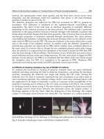
4.1 Binary axicon design
A classical cone axicon, introduced firstly by McLeod in 1954 (McLeod, 1954), is usually a
bulk one, as illustrated in Fig. 15(a), in which
D is the aperture diameter and
is the prism
angle. Based on binary optical ideas, the profile of a binary axicon, whose performance
required is equivalent to that of a bulk one, can be easily formed. Assuming straight-ray
propagation through the bulk axicon, the relation between the phase retardation
( )
and
the surface height
( )h
is given as (Feng et al., 2003)
2 1
( ) ( ) [( ) ]h n n k
(21)
where
k is the free space wave number,
1
n and
2
n are the refractive indexes of the air and the
axicon, respectively. To generate the continuous profile of the binary axicon, the equivalent
transformation can be used by (Hirayama et al., 1996)
2 1
( ) [ ( )mod 2 ] [( ) ]h n n k
(22)
The continuous profile of the binary axicon produced by (22) is shown in Fig. 15(c). For the
multilevel axicon, the profile is quantized into equal height step
. The quantized height is
given by
( ) int[ ( ) ]
q
h h
(23)
where
max
,h M
max 2 1
( )h n n
and
M
is the number of levels. Eq. (23) generates the
multilevel profiles of the binary axicon. The schematic diagram of the 4-level binary axicon
is illustrated in Fig. 15 (d). It is known that the larger the number of levels is, the higher the
diffraction efficiency is, however, the higher the difficulty of manufacture becomes.
Therefore, the compromise between the diffraction efficiency and the difficulty of
manufacture should be considered when determining the number of levels. In our work the
selection of the 32-level binary axicon is made. From Figs. 15(c) and 15(d), we can see easily
that the designed binary axicon is not only more compact than the classical cone axicon, but
also simpler to fabricate than the holographic axicon.
Fig. 15. The design process of a binary axicon. (a) A bulk axicon. (b) An axicon removed the
unwanted material (red part). (c) An equivalent binary axicon with continuous profile. (d)
An equivalent binary axicon quantized into four levels.
4.2 Rigorous electromagnetic analysis method
Because of rotational symmetry of the binary axicon, a 2-D FDTD method is applied to
evaluate the electromagnetic fields diffracted by the binary axicon in the near region. The
computational model of the 2-D FDTD method is shown schematically in Fig. 16, in which
the binary axicon is utilized to convert an incident beam into a pseudo-Bessel beam. To
stimulate the entire 2-D FDTD grid, a total-scattered field approach is applied to introduce a
normally incident plane wave. In this approach the connecting boundary serves to connect
the total and the scattered field regions, and is the location at which the incident field is
introduced. Because of the limitation of computational time and memory, the computational
range of the 2-D FDTD method is truncated by using perfectly matched layer (PML)
absorbing boundary conditions (ABCs) in the near region. Therefore, in order to accurately
determine the electromagnetic fields in the far region, Stratton-Chu integral formulas are
applied and given by (Stratton, 1941)
0 0 0
0 0 0
, , , '
, , , '
L
L
E r i n H r G r r n E r G r r n E r G r r dL
H r i n E r G r r n H r G r r n H r G r r dL
(24)
where ( , )r z
and ' ( ', ')r z
denote an arbitrary observation point in the far region and an
source point on the output boundary of the 2-D FDTD model, respectively; unit vector
n
is
the outer normal of the closed curve,
L
, of the output boundary;
(2)
0 0
, ( ) 4G r r iH k r r
, is the 2-D scalar Green’s function in free space,
(2)
0
H is the zero-
order Hankel function of the second kind and
k is the wave number in free space;
is the
angular frequency;
and
are the permittivity and permeability, respectively.
In short, our electromagnetic analysis method is to join the 2-D FDTD method for
computing the fields diffracted by the binary axicon in the near region with the Stratton-
Chu integral formulas for obtaining its diffractive fields in the far region. It can be
implemented by the following procedure: First, we carry out the 2-D FDTD computation
and obtain the near fields,
E r
and
H r
, on the output boundary. Then, these fields can
be regarded as secondary sources and substituted into (24) to calculate the fields,
E r
and
H r
, at arbitrary observation point in the far region. Note that the integral herein
is over the closed curve,
L
, of the output boundary.
Fig. 16. Schematic diagram of 2-D FDTD computational model, where the 8-level binary
axicon is embedded into FDTD grid.
4.3 Demonstration of equivalence
To demonstrate the equivalent performance between the bulk axicon and the designed
binary axicon, Fig. 17 shows the on-axis intensity distributions for both the bulk axicon and
the 32-level binary axicon. In this case both axicons, with the same aperture
Pseudo-BesselBeamsinMillimeterandSub-millimeterRange 485
4.1 Binary axicon design
A classical cone axicon, introduced firstly by McLeod in 1954 (McLeod, 1954), is usually a
bulk one, as illustrated in Fig. 15(a), in which
D is the aperture diameter and
is the prism
angle. Based on binary optical ideas, the profile of a binary axicon, whose performance
required is equivalent to that of a bulk one, can be easily formed. Assuming straight-ray
propagation through the bulk axicon, the relation between the phase retardation
( )
and
the surface height
( )h
is given as (Feng et al., 2003)
2 1
( ) ( ) [( ) ]h n n k
(21)
where
k is the free space wave number,
1
n and
2
n are the refractive indexes of the air and the
axicon, respectively. To generate the continuous profile of the binary axicon, the equivalent
transformation can be used by (Hirayama et al., 1996)
2 1
( ) [ ( )mod 2 ] [( ) ]h n n k
(22)
The continuous profile of the binary axicon produced by (22) is shown in Fig. 15(c). For the
multilevel axicon, the profile is quantized into equal height step
. The quantized height is
given by
( ) int[ ( ) ]
q
h h
(23)
where
max
,h M
max 2 1
( )h n n
and
M
is the number of levels. Eq. (23) generates the
multilevel profiles of the binary axicon. The schematic diagram of the 4-level binary axicon
is illustrated in Fig. 15 (d). It is known that the larger the number of levels is, the higher the
diffraction efficiency is, however, the higher the difficulty of manufacture becomes.
Therefore, the compromise between the diffraction efficiency and the difficulty of
manufacture should be considered when determining the number of levels. In our work the
selection of the 32-level binary axicon is made. From Figs. 15(c) and 15(d), we can see easily
that the designed binary axicon is not only more compact than the classical cone axicon, but
also simpler to fabricate than the holographic axicon.
Fig. 15. The design process of a binary axicon. (a) A bulk axicon. (b) An axicon removed the
unwanted material (red part). (c) An equivalent binary axicon with continuous profile. (d)
An equivalent binary axicon quantized into four levels.
4.2 Rigorous electromagnetic analysis method
Because of rotational symmetry of the binary axicon, a 2-D FDTD method is applied to
evaluate the electromagnetic fields diffracted by the binary axicon in the near region. The
computational model of the 2-D FDTD method is shown schematically in Fig. 16, in which
the binary axicon is utilized to convert an incident beam into a pseudo-Bessel beam. To
stimulate the entire 2-D FDTD grid, a total-scattered field approach is applied to introduce a
normally incident plane wave. In this approach the connecting boundary serves to connect
the total and the scattered field regions, and is the location at which the incident field is
introduced. Because of the limitation of computational time and memory, the computational
range of the 2-D FDTD method is truncated by using perfectly matched layer (PML)
absorbing boundary conditions (ABCs) in the near region. Therefore, in order to accurately
determine the electromagnetic fields in the far region, Stratton-Chu integral formulas are
applied and given by (Stratton, 1941)
0 0 0
0 0 0
, , , '
, , , '
L
L
E r i n H r G r r n E r G r r n E r G r r dL
H r i n E r G r r n H r G r r n H r G r r dL
(24)
where ( , )r z
and ' ( ', ')r z
denote an arbitrary observation point in the far region and an
source point on the output boundary of the 2-D FDTD model, respectively; unit vector
n
is
the outer normal of the closed curve,
L
, of the output boundary;
(2)
0 0
, ( ) 4G r r iH k r r
, is the 2-D scalar Green’s function in free space,
(2)
0
H is the zero-
order Hankel function of the second kind and
k is the wave number in free space;
is the
angular frequency;
and
are the permittivity and permeability, respectively.
In short, our electromagnetic analysis method is to join the 2-D FDTD method for
computing the fields diffracted by the binary axicon in the near region with the Stratton-
Chu integral formulas for obtaining its diffractive fields in the far region. It can be
implemented by the following procedure: First, we carry out the 2-D FDTD computation
and obtain the near fields,
E r
and
H r
, on the output boundary. Then, these fields can
be regarded as secondary sources and substituted into (24) to calculate the fields,
E r
and
H r
, at arbitrary observation point in the far region. Note that the integral herein
is over the closed curve,
L
, of the output boundary.
Fig. 16. Schematic diagram of 2-D FDTD computational model, where the 8-level binary
axicon is embedded into FDTD grid.
4.3 Demonstration of equivalence
To demonstrate the equivalent performance between the bulk axicon and the designed
binary axicon, Fig. 17 shows the on-axis intensity distributions for both the bulk axicon and
the 32-level binary axicon. In this case both axicons, with the same aperture
AdvancedMicrowaveandMillimeterWave
Technologies:SemiconductorDevices,CircuitsandSystems486
diameter
40D
and prism angle
0
10
, are normally illuminated by a plane wave of unit
amplitude. Other parameters used in Fig. 17 are as follows: an incident wavelength
is
0.32mm
(
0.94THzf
), the refractive indexes of the axicon and the air are
2
1.4491n
(Teflon) and
1
1.0n , respectively. Two distributions exhibit some differences in the near
region (
75z
). The reason is that the binary axicon suffers more from edge diffraction and
truncation effects (Trappe et al., 2005). The effects can also be seen from Fig. 18(b), which has
more burr than Fig. 18(a) in the near region. However, two curves show a good agreement
in the region ( 75z
), where the propagating beam can be best approximated by the Bessel
beam in terms of its intensity profile. Thus, the performance of the designed binary axicon is
equivalent to that of the bulk one. In order to further demonstrate the equivalent effect
between two axicons, we extend our 2-D FDTD calculated region to 200
along z-axis, and
display their electric-field amplitudes in a pseudo-color representation in Fig. 18. It can also
be seen that the designed binary axicon has the same performance as the bulk one.
Fig. 17. The axial intensity distributions for the designed binary axicon and the bulk one.
Fig. 18. Electric-field amplitude patterns plotted in a pseudo-color representation. (a) For the
bulk axicon. (b) For our designed binary axicon.
4.4 Properties of pseudo-Bessel beam
In order to study the properties of a pseudo-Bessel beam, the other 32-level binary axicon
having aperture diameter 44D
and prism angle
0
12
, are examined. Other parameters
used in this example are the same as in Fig .17. When this axicon is normally illuminated by
a plane wave of unit amplitude, its axial and transverse intensity distributions at three
representative values of
z :
max
0.8z Z
,
max
Z
and
max
1.2
Z
are shown in Figs. 19(a)-19(d),
respectively. It can be seen clearly from Fig. 19(a) that the on-axis intensity increases with
oscillating, and reaches its maximum axial intensity then decreases quickly, as the
propagation distance z increases. The maximum value of on-axis intensity in Fig. 19(a)
is
10.297 , located at
max
125.4Z
. As shown in Fig. 19(a), if
max
L
is defined as the maximum
propagation distance of a pseudo-Bessel beam, we can obtain
max
230L
. In addition,
according to geometrical optics (Trappe et al., 2005), a limited diffraction range
227L
is
estimated by:
L= D (2 tan )
and
1
sin( ) sinn
. We discover two results almost coincide.
From Figs. 19(b)-19(d) we can observe that their transverse intensity distributions are
approximations to Bessel function of the first kind. The radii of their central spot are only
about 3.5
. This indicates that the transverse intensity distribution of pseudo-Bessel beam is
highly localized. It is also interesting to point out that the radius size of
3.5
is very close to
the value of
3.4
, which is determined roughly from the first zero of the Bessel function
(
2.4048 (2 sin )
) (Trappe et al., 2005).
(a) (b)
(c) (d)
Fig. 19. The axial and transverse intensity distributions for the designed binary axicon. (a)
The on-axis intensity versus propagation distance
z . (b) The transverse intensity distribution
at
max
0.8z Z plane. (c)
max
1.0z Z
. (d)
max
1.2z Z
.
5. Propagation characteristic (Yu & Dou, 2008e)
The most interesting and attractive characteristic of Bessel beam is diffraction-free
propagation distance. In optics, the comparisons of maximum propagation distance had
been done between apertured Bessel and Gaussian beams by Durnin (Durnin, 1987; Durnin
et al., 1988) and Sprangle (Sprangle & Hafizi, 1991), respectively. However, the completely
Pseudo-BesselBeamsinMillimeterandSub-millimeterRange 487
diameter
40D
and prism angle
0
10
, are normally illuminated by a plane wave of unit
amplitude. Other parameters used in Fig. 17 are as follows: an incident wavelength
is
0.32mm
(
0.94THzf
), the refractive indexes of the axicon and the air are
2
1.4491n
(Teflon) and
1
1.0n , respectively. Two distributions exhibit some differences in the near
region (
75z
). The reason is that the binary axicon suffers more from edge diffraction and
truncation effects (Trappe et al., 2005). The effects can also be seen from Fig. 18(b), which has
more burr than Fig. 18(a) in the near region. However, two curves show a good agreement
in the region ( 75z
), where the propagating beam can be best approximated by the Bessel
beam in terms of its intensity profile. Thus, the performance of the designed binary axicon is
equivalent to that of the bulk one. In order to further demonstrate the equivalent effect
between two axicons, we extend our 2-D FDTD calculated region to 200
along z-axis, and
display their electric-field amplitudes in a pseudo-color representation in Fig. 18. It can also
be seen that the designed binary axicon has the same performance as the bulk one.
Fig. 17. The axial intensity distributions for the designed binary axicon and the bulk one.
Fig. 18. Electric-field amplitude patterns plotted in a pseudo-color representation. (a) For the
bulk axicon. (b) For our designed binary axicon.
4.4 Properties of pseudo-Bessel beam
In order to study the properties of a pseudo-Bessel beam, the other 32-level binary axicon
having aperture diameter 44D
and prism angle
0
12
, are examined. Other parameters
used in this example are the same as in Fig .17. When this axicon is normally illuminated by
a plane wave of unit amplitude, its axial and transverse intensity distributions at three
representative values of
z :
max
0.8z Z ,
max
Z
and
max
1.2
Z
are shown in Figs. 19(a)-19(d),
respectively. It can be seen clearly from Fig. 19(a) that the on-axis intensity increases with
oscillating, and reaches its maximum axial intensity then decreases quickly, as the
propagation distance z increases. The maximum value of on-axis intensity in Fig. 19(a)
is
10.297 , located at
max
125.4Z
. As shown in Fig. 19(a), if
max
L
is defined as the maximum
propagation distance of a pseudo-Bessel beam, we can obtain
max
230L
. In addition,
according to geometrical optics (Trappe et al., 2005), a limited diffraction range
227L
is
estimated by:
L= D (2 tan )
and
1
sin( ) sinn
. We discover two results almost coincide.
From Figs. 19(b)-19(d) we can observe that their transverse intensity distributions are
approximations to Bessel function of the first kind. The radii of their central spot are only
about 3.5
. This indicates that the transverse intensity distribution of pseudo-Bessel beam is
highly localized. It is also interesting to point out that the radius size of
3.5
is very close to
the value of
3.4
, which is determined roughly from the first zero of the Bessel function
(
2.4048 (2 sin )
) (Trappe et al., 2005).
(a) (b)
(c) (d)
Fig. 19. The axial and transverse intensity distributions for the designed binary axicon. (a)
The on-axis intensity versus propagation distance
z . (b) The transverse intensity distribution
at
max
0.8z Z plane. (c)
max
1.0z Z . (d)
max
1.2z Z .
5. Propagation characteristic (Yu & Dou, 2008e)
The most interesting and attractive characteristic of Bessel beam is diffraction-free
propagation distance. In optics, the comparisons of maximum propagation distance had
been done between apertured Bessel and Gaussian beams by Durnin (Durnin, 1987; Durnin
et al., 1988) and Sprangle (Sprangle & Hafizi, 1991), respectively. However, the completely
AdvancedMicrowaveandMillimeterWave
Technologies:SemiconductorDevices,CircuitsandSystems488
contrary conclusions were derived by them, owing to the difference between their contrast
criteria. Because Bessel beams have many potential applications at millimeter and sub-
millimeter wavebands, therefore, it is necessary and significant that the comparison is
carried out at these bands. A new comparison criterion in the spectrum of millimeter and
sub-millimeter range has been proposed by us. Under this criterion, the numerical results
obtained by using Stratton-Chu formulas instead of Fresnel-Kirchhoff diffraction integral
formula are presented; and a new conclusion is drawn.
5.1 Reviews of comparisons of Durnin and Sprangle
In this Subsection, the comparisons done by Durnin and Sprangle respectively are reviewed
at first. Because of the circular symmetries of Bessel and Gaussian beams, thus our
calculations are concerned only with circularly symmetric system. Let
( ',0)
and ( , )z
be the
coordinates of a pair of points on the incident and receive planes, respectively. In optics, it is
well known that scalar diffraction theory yields excellent results when the wavelength is
small compared with the size of the aperture and the propagation angles are not too steep
(Durnin, 1987). In the Fresnel approximation the amplitude
( , )
A
z
at a distance z can be
obtained from Fresnel-Kirchhoff diffraction integral formula (Jiang et al., 1995)
2 2
0
0
' '
( , ) exp( )( ) ( ',0) ( ) exp( ) 'd '
2 2
R
ik k k ik
A z ikz A J
z iz z z
(25)
where
2 2
x
y
,
2 2
' ' '
x
y
,
R
is the aperture radius of incident plane, and
0
2 2
0
( ') Bessel beam
( ',0)
exp( ' ) Gaussian beam
J k
A
w
(26)
for all
'
R
, and zero for all '
R
, where
k
is the radial wave number and
0
w
is the waist
radius of Gaussian beam. When 0
in (25), the axial intensity distribution (0, )
A
I z can be
given by
2
2
2
2
0
'
(0, ) (0, ) ( ',0) exp( ) 'd '
2
R
A
k ik
I z A z A
z z
(27)
According to Durnin’s comparison criterion (Durnin, 1987; Durnin et al., 1988) :
0 0
w
, that
is, on the incident plane (
' 0z ), the central spot radius
0
of zero-order Bessel beam
(i.e.
0
J
beam) is equal to the waist radius
0
w of Gaussian beam, as displayed in Fig. 20(a),
where
0 0
100w um
,
0
2.405k
, 2
R
mm , 0.6328um
, we calculate
the
(0, )
A
I z versus z curves by using (27), which are shown in Fig. 20(b). It can be seen clearly
from Fig. 20(b) that the Bessel beam propagates farther than the Gaussian beam.
However, according to Sprangle’s comparison criterion (Sprangle & Hafizi, 1991):
0
w R ,
and a
0
J
beam has at least one side-lobe on the incident plane, as illustrated in Fig. 21(a), we
can obtain the results given in Fig. 21(b). The converse conclusion that the Bessel beam
propagates no farther than the Gaussian beam can be easily drawn from Fig. 21(b).
(a) (b)
Fig. 20. The comparison of Durnin. (a) Intensity distributions for a
0
J
beam (—) and a
Gaussian beam ( ) on the incident plane where the beams are assumed to be formed. (b)
Axial intensities
(0, )
A
I z versus propagation distance z .
(a) (b)
Fig. 21. The comparison of Sprangle. (a) Intensity distributions for a
0
J
beam and a Gaussian
beam on the incident plane. (b) Axial intensities
(0, )
A
I z versus propagation distance z .
The reason why the converse conclusions were obtained by Durnin and Sprangle
respectively was that the criteria taken by them were very different. This fact can be seen
from Fig. 20(a) and Fig. 21(a). Moreover, the key problem of their criteria is not objective and
fair. Under Durnin’s criterion, the utilization ration of aperture for the Gaussian beam is
very low. In fact, we should not utilize so large aperture to eradiate a Gaussian beam with
so small waist radius. However, under Sprangle’s criterion, the powers carried by two
beams on the incident plane are not equal. Therefore, we propose a new comparison
criterion at millimeter wavelengths, which is discussed in the next Subsection.
5.2 Our comparison criterion and results
At millimeter wave bands, it is known that Fresnel-Kirchhoff diffraction integral formula
based on scalar theory is not suitable for calculating the diffractive field. The Stratton-Chu
formulas are one of the most powerful tools for the analysis of electromagnetic radiation
problems. So, they can be credibly used to determine the diffractive field, and rewritten as
(Stratton, 1941)
0 0 0
0 0 0
, , ,
, , ,
S
S
E r i n H r G r r n E r G r r n E r G r r dS
H r i n E r G r r n H r G r r n H r G r r dS
(28)
Pseudo-BesselBeamsinMillimeterandSub-millimeterRange 489
contrary conclusions were derived by them, owing to the difference between their contrast
criteria. Because Bessel beams have many potential applications at millimeter and sub-
millimeter wavebands, therefore, it is necessary and significant that the comparison is
carried out at these bands. A new comparison criterion in the spectrum of millimeter and
sub-millimeter range has been proposed by us. Under this criterion, the numerical results
obtained by using Stratton-Chu formulas instead of Fresnel-Kirchhoff diffraction integral
formula are presented; and a new conclusion is drawn.
5.1 Reviews of comparisons of Durnin and Sprangle
In this Subsection, the comparisons done by Durnin and Sprangle respectively are reviewed
at first. Because of the circular symmetries of Bessel and Gaussian beams, thus our
calculations are concerned only with circularly symmetric system. Let
( ',0)
and ( , )z
be the
coordinates of a pair of points on the incident and receive planes, respectively. In optics, it is
well known that scalar diffraction theory yields excellent results when the wavelength is
small compared with the size of the aperture and the propagation angles are not too steep
(Durnin, 1987). In the Fresnel approximation the amplitude
( , )
A
z
at a distance z can be
obtained from Fresnel-Kirchhoff diffraction integral formula (Jiang et al., 1995)
2 2
0
0
' '
( , ) exp( )( ) ( ',0) ( ) exp( ) 'd '
2 2
R
ik k k ik
A z ikz A J
z iz z z
(25)
where
2 2
x
y
,
2 2
' ' '
x
y
,
R
is the aperture radius of incident plane, and
0
2 2
0
( ') Bessel beam
( ',0)
exp( ' ) Gaussian beam
J k
A
w
(26)
for all
'
R
, and zero for all '
R
, where
k
is the radial wave number and
0
w
is the waist
radius of Gaussian beam. When 0
in (25), the axial intensity distribution (0, )
A
I z can be
given by
2
2
2
2
0
'
(0, ) (0, ) ( ',0) exp( ) 'd '
2
R
A
k ik
I z A z A
z z
(27)
According to Durnin’s comparison criterion (Durnin, 1987; Durnin et al., 1988) :
0 0
w
, that
is, on the incident plane (
' 0z
), the central spot radius
0
of zero-order Bessel beam
(i.e.
0
J
beam) is equal to the waist radius
0
w of Gaussian beam, as displayed in Fig. 20(a),
where
0 0
100w um
,
0
2.405k
, 2
R
mm
, 0.6328um
, we calculate
the
(0, )
A
I z versus z curves by using (27), which are shown in Fig. 20(b). It can be seen clearly
from Fig. 20(b) that the Bessel beam propagates farther than the Gaussian beam.
However, according to Sprangle’s comparison criterion (Sprangle & Hafizi, 1991):
0
w R ,
and a
0
J
beam has at least one side-lobe on the incident plane, as illustrated in Fig. 21(a), we
can obtain the results given in Fig. 21(b). The converse conclusion that the Bessel beam
propagates no farther than the Gaussian beam can be easily drawn from Fig. 21(b).
(a) (b)
Fig. 20. The comparison of Durnin. (a) Intensity distributions for a
0
J
beam (—) and a
Gaussian beam ( ) on the incident plane where the beams are assumed to be formed. (b)
Axial intensities
(0, )
A
I z versus propagation distance z .
(a) (b)
Fig. 21. The comparison of Sprangle. (a) Intensity distributions for a
0
J
beam and a Gaussian
beam on the incident plane. (b) Axial intensities
(0, )
A
I z versus propagation distance z .
The reason why the converse conclusions were obtained by Durnin and Sprangle
respectively was that the criteria taken by them were very different. This fact can be seen
from Fig. 20(a) and Fig. 21(a). Moreover, the key problem of their criteria is not objective and
fair. Under Durnin’s criterion, the utilization ration of aperture for the Gaussian beam is
very low. In fact, we should not utilize so large aperture to eradiate a Gaussian beam with
so small waist radius. However, under Sprangle’s criterion, the powers carried by two
beams on the incident plane are not equal. Therefore, we propose a new comparison
criterion at millimeter wavelengths, which is discussed in the next Subsection.
5.2 Our comparison criterion and results
At millimeter wave bands, it is known that Fresnel-Kirchhoff diffraction integral formula
based on scalar theory is not suitable for calculating the diffractive field. The Stratton-Chu
formulas are one of the most powerful tools for the analysis of electromagnetic radiation
problems. So, they can be credibly used to determine the diffractive field, and rewritten as
(Stratton, 1941)
0 0 0
0 0 0
, , ,
, , ,
S
S
E r i n H r G r r n E r G r r n E r G r r dS
H r i n E r G r r n H r G r r n H r G r r dS
(28)
AdvancedMicrowaveandMillimeterWave
Technologies:SemiconductorDevices,CircuitsandSystems490
where
( , )r z
, ' ( ',0)r
,
0
, (4 )
ik r r
G r r e r r
, is the scalar Green’s function. Let
us assume that on the incident plane (
' 0z ) we have a
0
J
beam and a Gaussian beam,
polarized in the
x
direction and propagating in the z direction. They are expressed in the
following forms, respectively.
0 0
2 2 2 2
0 0
( ') ( '), ( ') ( ') Bessel beam
( ') exp( ' ), ( ') exp( ' ) Gaussian beam
E r xJ k H r y J k
E r x w H r y w
(29)
where
. When
0
in (28), the axial intensity distribution (0, )
A
I z can be obtained by
substituting (29) into (28)
2 2
(0, ) ( ) (0, )
A
I z E r E z
(30)
In addition, at a certain plane
f
z z , the transverse intensity distribution ( , )
T f
I z
can also
be calculated by
2 2
( , ) ( ) ( , )
T f f
I z E r E z
(31)
Now, we propose our contrast criterion: the same initial total power and central peak
intensity on the same initial aperture. In order to compare conveniently, we also defined the
propagation distance as the value of z-axis at which the axial intensity falls to
1 2 . Three
cases are presented herein, where the same parameters are
3mm
and 10R
. In the first
example, their intensity distributions for a
0
J
beam and a Gaussian beam on the initial
aperture are shown in Fig. 22(a). Using (30), we get the axial intensity distributions along z-
axis, as illustrated in Fig. 22(b). For the purpose of observing the propagation process, Figs.
22(c)-22(f) display the transverse intensity distributions at
10 , 20 ,30 ,40z
, respectively.
From this instance, A conclusion can be easily reach that the propagation distance of
the
0
J
beam is greater than that of the Gaussian beam, under the condition of the same initial
total power and central peak intensity on the same initial aperture. In order to further
confirm our conclusion, the other two examples are presented in Fig. 23 and Fig. 24.
Apparently, a similar conclusion can be drawn from Figs. 23 and 24.
From Figs. 22(b), 23(b) and 24(b), we can also observe that the axial intensity distributions of
Bessel beams oscillate more acutely than those of Gaussian beams. This is because the initial
field distributions of Bessel beams near the edges of the aperture are much larger than those
of Gaussian beams, and as a result, Bessel beam will suffer more diffraction on the sharp
edges of the aperture than Gaussian beams.
(a) (b)
(c) (d)
(e) (f)
Fig. 22. The first case. (a) Intensity distributions for an apertured Bessel beam (—) and an
apertured Gaussian beam ( ) on the incident plane. (b) Axial intensities
(0, )
A
I z versus
propagation distance
z . (c)-(f) Transverse intensity distributions at
10 , 20 ,30 ,40z
,
respectively.
(a) (b)
Fig. 23. The second case. (a) Initial Intensity distributions on the incident plane. (b) Axial
intensities
(0, )
A
I z versus propagation distance z .
(a) (b)
Fig. 24. The last case. (a) Intensity intensity distributions on the apture. (b) Their
propagation distance.
Pseudo-BesselBeamsinMillimeterandSub-millimeterRange 491
where
( , )r z
, ' ( ',0)r
,
0
, (4 )
ik r r
G r r e r r
, is the scalar Green’s function. Let
us assume that on the incident plane (
' 0z
) we have a
0
J
beam and a Gaussian beam,
polarized in the
x
direction and propagating in the z direction. They are expressed in the
following forms, respectively.
0 0
2 2 2 2
0 0
( ') ( '), ( ') ( ') Bessel beam
( ') exp( ' ), ( ') exp( ' ) Gaussian beam
E r xJ k H r y J k
E r x w H r y w
(29)
where
. When
0
in (28), the axial intensity distribution (0, )
A
I z can be obtained by
substituting (29) into (28)
2 2
(0, ) ( ) (0, )
A
I z E r E z
(30)
In addition, at a certain plane
f
z z
, the transverse intensity distribution ( , )
T f
I z
can also
be calculated by
2 2
( , ) ( ) ( , )
T f f
I z E r E z
(31)
Now, we propose our contrast criterion: the same initial total power and central peak
intensity on the same initial aperture. In order to compare conveniently, we also defined the
propagation distance as the value of z-axis at which the axial intensity falls to
1 2 . Three
cases are presented herein, where the same parameters are
3mm
and 10R
. In the first
example, their intensity distributions for a
0
J
beam and a Gaussian beam on the initial
aperture are shown in Fig. 22(a). Using (30), we get the axial intensity distributions along z-
axis, as illustrated in Fig. 22(b). For the purpose of observing the propagation process, Figs.
22(c)-22(f) display the transverse intensity distributions at
10 , 20 ,30 ,40z
, respectively.
From this instance, A conclusion can be easily reach that the propagation distance of
the
0
J
beam is greater than that of the Gaussian beam, under the condition of the same initial
total power and central peak intensity on the same initial aperture. In order to further
confirm our conclusion, the other two examples are presented in Fig. 23 and Fig. 24.
Apparently, a similar conclusion can be drawn from Figs. 23 and 24.
From Figs. 22(b), 23(b) and 24(b), we can also observe that the axial intensity distributions of
Bessel beams oscillate more acutely than those of Gaussian beams. This is because the initial
field distributions of Bessel beams near the edges of the aperture are much larger than those
of Gaussian beams, and as a result, Bessel beam will suffer more diffraction on the sharp
edges of the aperture than Gaussian beams.
(a) (b)
(c) (d)
(e) (f)
Fig. 22. The first case. (a) Intensity distributions for an apertured Bessel beam (—) and an
apertured Gaussian beam ( ) on the incident plane. (b) Axial intensities (0, )
A
I z versus
propagation distance
z . (c)-(f) Transverse intensity distributions at
10 , 20 ,30 ,40z
,
respectively.
(a) (b)
Fig. 23. The second case. (a) Initial Intensity distributions on the incident plane. (b) Axial
intensities
(0, )
A
I z versus propagation distance z .
(a) (b)
Fig. 24. The last case. (a) Intensity intensity distributions on the apture. (b) Their
propagation distance.
AdvancedMicrowaveandMillimeterWave
Technologies:SemiconductorDevices,CircuitsandSystems492
6. Applications and Conclusions
The novel properties of the diffraction-free Bessel beams have many significant applications
(Bouchal, 2003). In optics, due to the propagation invariance and extremely narrow intensity
profile, Bessel beams are applicable in metrology for scanning optical systems. These beams
are also suitable for large-scale straightness and measurements (Wang et al., 2003), since
they can stand the atmospheric turbulence more than other beams. The imaging
applications of the diffraction-free Bessel beams are also presented in (Li & Aruga, 1999),
and it has been demonstrated that the imaging produced by Bessel beams can provide a
longer focal depth when compared with Gaussian beams. Bessel beams can also be applied
to optical interconnection and promotion of free electron laser gain (Li et al., 2006). An
increasing attention is devoted to the applications of Bessel beams in nonlinear optics. The
third-harmonic generation using Bessel beams was proposed by Tewari and co-workers
(Tewari et al., 1996). In addition, Cerenkov second-harmonic generation by nondiffracting
Bessel beams in bulk optical crystals was also suggested in (Pandit & Payne, 1997). The
application of Bessel beams to increase the Z-scan sensitivity in measurement was
demonstrated in (Hughes & Burzler, 1997). The radially polarized Bessel beams were
applicable to accelerate the particles of the electron beam (Tidwell et al., 1992). Recently,
Bessel beams are used to manipulate micrometer-sized particles. Using the self-
reconstruction property of Bessel beam, it is possible to manipulate tiny particles
simultaneously in multiple planes (Hegner, 2002; Garces-Chavez et al., 2002). We believe
that Bessel beams are prospective for improving the resolution of images in millimeter wave
imaging system (Monk, 1999). These beams may also be useful for measurements and
power transmission at millimeter and sub-millimeter wavebands.
In optical region of the spectrum, diffraction-free Bessel beams have attracted much interest
over the years and have been widely investigated. However, in the millimeter and sub-
millimeter wave regions, exploratory work devoted to this field is much less. So, a great deal
of contribution should be made to this field in the future.
7. Acknowledgments
This work is supported by NSFC under grant 60621002, the Natural Science Foundation of
Fujian Province of China (No.A0610027) and the Key Project of Quanzhou City Science and
Technology Program (No.2008G13).
8. References
Arlt, J. & Dholakia, K. (2000). Generation of high-order Bessel beams by use of an axicon.
Opt. Commun., Vol. 177, pp. 297-301
Bouchal, Z.; Wagner, J. & Chlup, M. (1998). Self-reconstruction of a distorted nondiffracting
beam. Opt. Commun., Vol. 151, No. 4-6, pp. 207–211
Bouchal, Z. (2003). Nondiffracting optical beams: physical properties, experiments, and
applications. Czech. J. phys., Vol. 53, No. 7, pp. 537-624
Cox, A. J. & Dibble, D. C. (1992). Nondiffracting beam from a spatially filtered Fabry-Perot
resonator. J. Opt. Soc. Am. A, Vol. 9, No. 2, pp. 282–286
Cong, W. X.; Chen, N. X. & Gu, B. Y. (1998). Generation of nondiffracting beams by
diffractive phase elements. J. Opt. Soc. Am. A, Vol. 15, No. 9, pp. 2362–2364
Courtial, J.; Whyte, G.; Bouchal, Z.; et al. (2006). Iterative algorithms for holographic shaping
of non-diffracting and self-imaging light beams. Opt. Express, Vol. 14, No. 6, pp.
2108–2116
Durnin, J. (1987). Exact solutions for nondiffracting beams. I. The scalar theory. J. Opt. Soc.
Am. A, Vol. 4, No. 4, pp. 651–654
Durnin, J.; Miceli J. J., Jr. & Eberly, J. H. (1987). Diffraction-free beams. Phys. Rev. Lett., Vol.
58, No. 15, pp. 1499-1501
Feng, D.; Yan, Y. B.; Jin, G. F.; et al. (2003). Rigorous electromagnetic design of finite-
aperture diffractive optical elements by use of an iterative optimization algorithm.
J. Opt. Soc. Am. A, Vol. 20, No. 9, pp. 1739-1745
Garces-Chavez, V.; Mcgloin, D. & Melvill, E. H. (2002). Simultaneous micromanipulation in
multiple planes using a self-reconstructing light beam. Nature, Vol. 419, No. 6903,
pp. 145–147
Haupt, R. L. (1995). An introduction to genetic algorithms for electromagnetics. IEEE
Antennas Propag. Mag., Vol. 37, No. 2, pp. 7-15
Hirayama, K.; Glytsis, E. N. & Gaylord, T. K. (1996). Rigorous electromagnetic analysis of
diffractive cylindrical lenses. J. Opt. Soc. Am. A, Vol. 13, No. 11, pp. 2219–2231
Hughes, S. & Burzler, J. M. (1997). Theory of Z-scan measurements using Gaussian-Bessel
beams. Phys. Rev. A, Vol. 56, No. 2, pp. R1103–R1106
Hegner, M. (2002). Optics: The light fantastic. Nature, Vol. 419, No. 6903, pp. 125–127
Jiang, Z. P.; Lu, Q. S. & Liu, Z. J. (1995). Propagation of apertured Bessel beam. Appl. Opt.,
Vol. 34, No. 31, pp. 7183-7185
Li, S. W. & Aruga, T. (1999). Long focal depth imaging over a long range. J. Commun. Res.
Lab., Vol. 46, No. 3, pp. 309–310
Li, D.; Imasaki, K.; Miyamoto, S.; et al. (2006). Conceptual design of Bessel beam cavity for
free-electron laser. Int. J. Infrared Millim. Waves, Vol. 27, No. 2, pp. 165-171
McLeod, J. H. (1954). The axicon: a new type of optical element. J. Opt. Soc. Am, Vol. 44, No.
8, pp. 592–597
MacDonald, R. P.; Boothroyd, S. A.; Okamoto, T.; et al. (1996). Interboard optical data
distribution by Bessel beam shadowing. Opt. Commun., Vol. 122, No. 4-6, pp. 169–77
Miceli J. J., Jr. & Eberly, J. H. (1988). Comparison of Bessel and Gaussian beams. Opt. Lett.,
Vol. 13, No. 2, pp. 79-80
Monk, S.; Arlt, J.; Robertson, D. A.; et al. (1999). Generation of Bessel beams at millimetre-
wave frequencies by use of an axicon. Opt. Commun., Vol. 170, pp. 213-215
Meltaus, J.; Salo, J.; Noponen, E.; et al. (2003). Millimeter-wave beam shaping using
holograms. IEEE Trans. Microwave Theory Tech., Vol. 51, No. 4, pp.1274-1279
Mahon, R. J.; Lanigan, W.; Murphy, J. A.; et al. (2005). Novel techniques for millimeter wave
imaging systems operating at 100GHz. Proc. SPIE. Int. Soc. Opt. Eng., Vol. 5789, pp.
93-100
McGloin, D. & Dholakia, K. (2005). Bessel beams: diffraction in a new light.
Contemp. Phys.,
Vol. 46, No. 1, pp. 15–28
Pandit M. K. & Payne, F. P. (1997). Cerenkov second-harmonic generation by nondiffracting
Bessel beams in bulk optical crystals. Opt. Quantum Electron., Vol. 29, No. 1, pp. 35–
51
Pseudo-BesselBeamsinMillimeterandSub-millimeterRange 493
6. Applications and Conclusions
The novel properties of the diffraction-free Bessel beams have many significant applications
(Bouchal, 2003). In optics, due to the propagation invariance and extremely narrow intensity
profile, Bessel beams are applicable in metrology for scanning optical systems. These beams
are also suitable for large-scale straightness and measurements (Wang et al., 2003), since
they can stand the atmospheric turbulence more than other beams. The imaging
applications of the diffraction-free Bessel beams are also presented in (Li & Aruga, 1999),
and it has been demonstrated that the imaging produced by Bessel beams can provide a
longer focal depth when compared with Gaussian beams. Bessel beams can also be applied
to optical interconnection and promotion of free electron laser gain (Li et al., 2006). An
increasing attention is devoted to the applications of Bessel beams in nonlinear optics. The
third-harmonic generation using Bessel beams was proposed by Tewari and co-workers
(Tewari et al., 1996). In addition, Cerenkov second-harmonic generation by nondiffracting
Bessel beams in bulk optical crystals was also suggested in (Pandit & Payne, 1997). The
application of Bessel beams to increase the Z-scan sensitivity in measurement was
demonstrated in (Hughes & Burzler, 1997). The radially polarized Bessel beams were
applicable to accelerate the particles of the electron beam (Tidwell et al., 1992). Recently,
Bessel beams are used to manipulate micrometer-sized particles. Using the self-
reconstruction property of Bessel beam, it is possible to manipulate tiny particles
simultaneously in multiple planes (Hegner, 2002; Garces-Chavez et al., 2002). We believe
that Bessel beams are prospective for improving the resolution of images in millimeter wave
imaging system (Monk, 1999). These beams may also be useful for measurements and
power transmission at millimeter and sub-millimeter wavebands.
In optical region of the spectrum, diffraction-free Bessel beams have attracted much interest
over the years and have been widely investigated. However, in the millimeter and sub-
millimeter wave regions, exploratory work devoted to this field is much less. So, a great deal
of contribution should be made to this field in the future.
7. Acknowledgments
This work is supported by NSFC under grant 60621002, the Natural Science Foundation of
Fujian Province of China (No.A0610027) and the Key Project of Quanzhou City Science and
Technology Program (No.2008G13).
8. References
Arlt, J. & Dholakia, K. (2000). Generation of high-order Bessel beams by use of an axicon.
Opt. Commun., Vol. 177, pp. 297-301
Bouchal, Z.; Wagner, J. & Chlup, M. (1998). Self-reconstruction of a distorted nondiffracting
beam. Opt. Commun., Vol. 151, No. 4-6, pp. 207–211
Bouchal, Z. (2003). Nondiffracting optical beams: physical properties, experiments, and
applications. Czech. J. phys., Vol. 53, No. 7, pp. 537-624
Cox, A. J. & Dibble, D. C. (1992). Nondiffracting beam from a spatially filtered Fabry-Perot
resonator. J. Opt. Soc. Am. A, Vol. 9, No. 2, pp. 282–286
Cong, W. X.; Chen, N. X. & Gu, B. Y. (1998). Generation of nondiffracting beams by
diffractive phase elements. J. Opt. Soc. Am. A, Vol. 15, No. 9, pp. 2362–2364
Courtial, J.; Whyte, G.; Bouchal, Z.; et al. (2006). Iterative algorithms for holographic shaping
of non-diffracting and self-imaging light beams. Opt. Express, Vol. 14, No. 6, pp.
2108–2116
Durnin, J. (1987). Exact solutions for nondiffracting beams. I. The scalar theory. J. Opt. Soc.
Am. A, Vol. 4, No. 4, pp. 651–654
Durnin, J.; Miceli J. J., Jr. & Eberly, J. H. (1987). Diffraction-free beams. Phys. Rev. Lett., Vol.
58, No. 15, pp. 1499-1501
Feng, D.; Yan, Y. B.; Jin, G. F.; et al. (2003). Rigorous electromagnetic design of finite-
aperture diffractive optical elements by use of an iterative optimization algorithm.
J. Opt. Soc. Am. A, Vol. 20, No. 9, pp. 1739-1745
Garces-Chavez, V.; Mcgloin, D. & Melvill, E. H. (2002). Simultaneous micromanipulation in
multiple planes using a self-reconstructing light beam. Nature, Vol. 419, No. 6903,
pp. 145–147
Haupt, R. L. (1995). An introduction to genetic algorithms for electromagnetics. IEEE
Antennas Propag. Mag., Vol. 37, No. 2, pp. 7-15
Hirayama, K.; Glytsis, E. N. & Gaylord, T. K. (1996). Rigorous electromagnetic analysis of
diffractive cylindrical lenses. J. Opt. Soc. Am. A, Vol. 13, No. 11, pp. 2219–2231
Hughes, S. & Burzler, J. M. (1997). Theory of Z-scan measurements using Gaussian-Bessel
beams. Phys. Rev. A, Vol. 56, No. 2, pp. R1103–R1106
Hegner, M. (2002). Optics: The light fantastic. Nature, Vol. 419, No. 6903, pp. 125–127
Jiang, Z. P.; Lu, Q. S. & Liu, Z. J. (1995). Propagation of apertured Bessel beam. Appl. Opt.,
Vol. 34, No. 31, pp. 7183-7185
Li, S. W. & Aruga, T. (1999). Long focal depth imaging over a long range. J. Commun. Res.
Lab., Vol. 46, No. 3, pp. 309–310
Li, D.; Imasaki, K.; Miyamoto, S.; et al. (2006). Conceptual design of Bessel beam cavity for
free-electron laser. Int. J. Infrared Millim. Waves, Vol. 27, No. 2, pp. 165-171
McLeod, J. H. (1954). The axicon: a new type of optical element. J. Opt. Soc. Am, Vol. 44, No.
8, pp. 592–597
MacDonald, R. P.; Boothroyd, S. A.; Okamoto, T.; et al. (1996). Interboard optical data
distribution by Bessel beam shadowing. Opt. Commun., Vol. 122, No. 4-6, pp. 169–77
Miceli J. J., Jr. & Eberly, J. H. (1988). Comparison of Bessel and Gaussian beams. Opt. Lett.,
Vol. 13, No. 2, pp. 79-80
Monk, S.; Arlt, J.; Robertson, D. A.; et al. (1999). Generation of Bessel beams at millimetre-
wave frequencies by use of an axicon. Opt. Commun., Vol. 170, pp. 213-215
Meltaus, J.; Salo, J.; Noponen, E.; et al. (2003). Millimeter-wave beam shaping using
holograms. IEEE Trans. Microwave Theory Tech., Vol. 51, No. 4, pp.1274-1279
Mahon, R. J.; Lanigan, W.; Murphy, J. A.; et al. (2005). Novel techniques for millimeter wave
imaging systems operating at 100GHz. Proc. SPIE. Int. Soc. Opt. Eng., Vol. 5789, pp.
93-100
McGloin, D. & Dholakia, K. (2005). Bessel beams: diffraction in a new light.
Contemp. Phys.,
Vol. 46, No. 1, pp. 15–28
Pandit M. K. & Payne, F. P. (1997). Cerenkov second-harmonic generation by nondiffracting
Bessel beams in bulk optical crystals. Opt. Quantum Electron., Vol. 29, No. 1, pp. 35–
51
AdvancedMicrowaveandMillimeterWave
Technologies:SemiconductorDevices,CircuitsandSystems494
Stratton, J. A. (1941). Electromagnetic Theory. McGraw-Hill, NewYork
Sprangle P. & Hafizi, B. (1991). Comment on nondiffracting beams. Phys. Rev. Lett., Vol. 66,
No. 6, pp. 837
Scott, G. & McArdle, N. (1992). Efficient generation of nearly diffraction-free beams using an
axicon. Opt. Eng, Vol. 31, No. 12, pp. 2640-2643
Salo, J.; Meltaus, J.; Noponen, E.; et al. (2001). Millimetre-wave Bessel beams using computer
holograms. Electron. Lett., Vol. 37, No. 13, pp. 834–835
Tidwell, S. C.; Ford, D. H. & Kimura, W. D. (1992). Transporting and focusing radially
polarized laser beams. Opt. Eng., Vol. 31, No. 7, pp. 1527–1531
Tewari, S. P.; Huang, H. & Boyd, R. W. (1996). Theory of third-harmonic generation using
Bessel beams, and self-phase-matching. Phys. Rev. A, Vol. 54, No. 3, pp. 2314–2325
Turunen, J.; Vasara, A. & Friberg, A. T. (1988). Holographic generation of diffraction-free
beams. Appl. Opt., Vol. 27, No. 19, pp. 3959–3962
Thewes, K.; Karim, M. A. & Awwal, A. A. S. (1991). Diffraction free beam generation using
refracting systems. Opt. Laser Technol., Vol. 23, No. 2, pp. 105–108
Trappe, N.; Mahon, R.; Lanigan, W.; et al. (2005). The quasi-optical analysis of Bessel beams
in the far infrared. Infrared Phys. Technol., Vol. 46, pp. 233–247
Weile, D. S. & Michielssen, E. (1997). Genetic algorithm optimization applied to
electromagnetics: A review. IEEE Trans. Antennas Propag., Vol. 45, No. 3, pp. 343-
353
Wang, K.; Zeng, L. & Yin, Ch. (2003). Influence of the incident wave-front on intensity
distribution of the nondiffracting beam used in large-scale measurement. Opt.
Commun., Vol. 216, No. 1–3, pp. 99–103
Yee, K. S. (1966). Numerical solution of initial boundary value problems involving Maxwell
equations in isotropic media. IEEE Trans. Antennas Propag., Vol. AP-14, No. 3, pp.
302-307
Yu, Y. Z. & Dou, W. B. (2008a). Scalar and vectorial properties of diffraction-free Bessel
beams. 2008 Asia Pacific Microwave Conference, APMC2008, Hongkong & Macau,
China.
Yu, Y. Z. & Dou, W. B. (2008b). Vector analyses of nondiffracting Bessel beams. Progress In
Electromagnetics Research Letters, Vol. 5, pp. 57–71
Yu, Y. Z. & Dou, W. B. (2008c). Generation of Bessel beams at mm- and submm-wave bands
using binary optical elements. 2008 Global Symp. on Millimeter Waves Proc., Nanjing,
China, pp. 115–118.
Yu, Y. Z. & Dou, W. B. (2008d). Generation of Bessel beams at mm- and sub mm-
wavelengths by binary optical elements. Int. J. Infrared Milli. Waves, Vol. 29, No. 7,
pp. 693–703
Yu, Y. Z. & Dou, W. B. (2008e). Comparison of propagation of apertured Bessel and
Gaussian beams. 2008 Int. Conf. Commun. Technol. Proc., Hangzhou, China, pp. 217–
220
Yu, Y. Z. & Dou, W. B. (2009). Generation of pseudo-Bessel beams at THz frequencies by use
of binary axicons. Opt. Express, Vol. 17, No. 2, pp. 888-893
ReceiverFront-EndArchitectures–AnalysisandEvaluation 495
ReceiverFront-EndArchitectures–AnalysisandEvaluation
PedroCruz,HugoGomesandNunoCarvalho
X
Receiver Front-End
Architectures – Analysis and Evaluation
Pedro Cruz
#
, Hugo Gomes
#
* & Nuno Carvalho
#
#
Universidade de Aveiro (Instituto de Telecomunicações)
Aveiro, Portugal
*Instituto Politécnico de Leiria (ESTG)
Leiria, Portugal
1. Introduction
In today's world, the exponential growth from communications between people/companies
in different places (at same time), the increasing requirement to measure and control all
processes, the analysis in real time, the mandatory requirement to provide of information
and entertainment data to electronic devices that must be increasingly smaller and more
complex, requires a continuous and nonstop searching for new technologies with greater
capacity, lower cost, reduced size and improved reliability.
The communications systems based on radio-frequency (RF) transmission are one of the
greatest examples of this challenging demand. These systems, present in almost all
equipment used in daily life as mobile phones, notebooks, wireless sensors, among other,
require an increasing versatility and ability to storage of data, huge transmission rates of
information and size reduction.
All this need for more sophisticated equipment, along with a greater number of services
available in a single equipment (preferably portable), besides the drastic size reductions
from the electronic components, requires a constant search for new architectures and new
materials in order to maximize the features offered.
One of the most important parts from a RF system device is this receiver architecture. In
receivers, the entry block has a key role in performance and reliability of the system. Any
unresolved issue caused by this block, generates enormous problems in the following blocks
of the receiver’s architecture. For this reason, considering the constant increase of services
available for the same frequency bands, associated with the growing number of users for
each service, the entry receiver architecture must be capable to resolve issues such as
blocking problems, peak-to-average power ratio (PAPR) problems, among others. In other
hand, must be capable to offer good selectivity, sensitivity, lower energy consumption for a
small price.
This chapter is organized in the following way. Firstly, a general review about the most
common receiving architectures is done, emphasizing its main advantages and drawbacks.
Moreover, some enhancements to these architectures are also presented and its principal
benefits are explained, such as Hartley and Weaver configurations. This section ends with
25