Advances in Haptics Part 9 docx

Bạn đang xem bản rút gọn của tài liệu. Xem và tải ngay bản đầy đủ của tài liệu tại đây (3.94 MB, 40 trang )

AdvancesinHaptics312

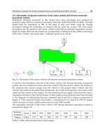
Fig. 12. A burr-tool receiving force-feedback from a polygonized pelvis model where the
force (direction and strength) is displayed with a blue line

At present, users are unable to distinguish between most different types of material textures
while using the voxel-only approach to collision detection. This is largely due to the discrete
nature of voxels promoting a “blocky” surface contact with the spherical burr. This issue
could be partially addressed by increasing the voxel density used to represent and object
volume. However, this solution becomes resource demanding past a certain point. The
collision detection method that exploits the mesh feels much smoother when passing over
flat and rounded surfaces with the burr; however different material haptic surface textures
have not yet been convincingly implemented.

6. Discussion
Both the Dynamic Ball Pivoting Algorithm and Haptic system need to mature into more
robust versions of their current selves before their inherent potential can truly shine through.
Also, while basing the haptic class’ force equation on Hooke’s law is convenient, it is also
inaccurate. A more involved and realistic model would be to use a material’s full stress-
strain curve0 to dictate the amount of force required to remove volume from the model.
However, such a change would require a means to measure to amount of force the user is
exerting on the haptic device.
A question that has come up before is: why we bother with the anchor-based method for
finding the force direction when we could use the nearest colliding voxel or use the
summation of the direction vectors of all voxels colliding with the burr-head instead? The
reason for this is that the nearest-voxel or voxel-summation methods have shown to
perform erratically whenever the burr-head is placed in a tight corner or inside a pit. On the
other hand, the anchor-based method has shown to perform as expected in both these
situations as well as on normal surface curvatures.

7. Conclusion and Future Work
This new system adds a sense of touch to the process of removing volume from voxelized
objects and is built on top of William et al.’s graphical carving simulator. Two components
operate in unison in order to make this work: an OpenSceneGraph thread and a haptic
thread. The former is responsible for clearing voxels queued for removal, redrawing the
scene and providing the haptic thread with a subset of the object data; the voxels and
triangles most likely to be relevant during collision detection are cached here. The latter
deals with issuances of both the direction and magnitude of force as well as evaluating
which sections of volume should be removed from the object.
There are certainly a great many directions where the haptic portion of the system can be
improved and extended in the future. One area that would improve the program’s use
would be to have a more modular approach to the cutting tools. Tools other than a burr
with a spherical head are likely to be useful to surgeons. The head may instead be an
ellipsoid, conical or cylindrical. The cutting tool could also be something non-motorized
such a scalpel which would require the distinction between cutting surfaces and non-cutting
surfaces to be made.
At the moment, models have a global ultimate strength value meaning that all the voxel will
have the same stiffness. In many cases, such as our target example; operating on human
bone, this is unrealistic as their exteriors are made of dense cortical bone while their interior
is composed of much softer bone marrow. Assigning each voxel its own density value is our
next step. This will also allow us to examine a voxel removal strategy whereby the act of
“cutting” an object will incrementally reduce the voxels density and voxels finding
themselves with a density of zero are considered wholly “cut”. The same idea can be
extended to the mesh-based collision detection. The hope is that this will allow a user to feel
a more progressive entry into an object while it is being cut.

8. References
[1] Williams J, Telles O’Neill G, Lee WS. Interactive 3d haptic carving using combined
voxels and mesh. Haptic Audio visual Environments and Games, 2008. HAVE
2008; pp 108-113, DOI: 10.1109/HAVE.2008.4685308

[2] Kim L, Park SH. Haptic interaction and volume modeling techniques for realistic dental
simulation. The visual Computer: International Journal of Computer Graphics.
Volume 22, Issue 2, 2006; pp 90-98, DOI: 10.1007/s00371-006-0369-8
[3] Yau HT, Tsou LS, Tsai MJ. Octree-based Virtual Dental Training System with a Haptic
Device. Computer-Aided Design & Applications. Volume 3, 2006; pp 415-424
[4] Agus M, Giachetti A, Gobbetti E, Zanetti G, Zorcolo A. Real-time haptic and visual
simulation of bone dissection. Presence: Teleoperators and Virtual Environments;
special issue: IEEE virtual reality 2002 conference; Volume 12, Issue 1, 2003; pp 110-
122
[5] Agus M, Giachetti A, Gobbetti E, Zanetti G, Zorcolo A. Adaptive techniques for real-time
haptic and visual simulation of bone dissection. Virtual Reality, 2003. Proceedings.
IEEE; pp 102-109, DOI: 10.1109/VR.2003.1191127
[6] Bernardini F, Mittleman J, Rushmeir H, Silva C, Taubin. The ball-pivoting algorithm for
surface reconstruction. Visualization and Computer Graphics, Volume 5, Issue 4,
1999; pp 349-359, DOI: 10.1109/2945.817351
Haptic-Based3DCarvingSimulator 313

Fig. 12. A burr-tool receiving force-feedback from a polygonized pelvis model where the
force (direction and strength) is displayed with a blue line

At present, users are unable to distinguish between most different types of material textures
while using the voxel-only approach to collision detection. This is largely due to the discrete
nature of voxels promoting a “blocky” surface contact with the spherical burr. This issue
could be partially addressed by increasing the voxel density used to represent and object
volume. However, this solution becomes resource demanding past a certain point. The
collision detection method that exploits the mesh feels much smoother when passing over
flat and rounded surfaces with the burr; however different material haptic surface textures
have not yet been convincingly implemented.

6. Discussion

Both the Dynamic Ball Pivoting Algorithm and Haptic system need to mature into more
robust versions of their current selves before their inherent potential can truly shine through.
Also, while basing the haptic class’ force equation on Hooke’s law is convenient, it is also
inaccurate. A more involved and realistic model would be to use a material’s full stress-
strain curve0 to dictate the amount of force required to remove volume from the model.
However, such a change would require a means to measure to amount of force the user is
exerting on the haptic device.
A question that has come up before is: why we bother with the anchor-based method for
finding the force direction when we could use the nearest colliding voxel or use the
summation of the direction vectors of all voxels colliding with the burr-head instead? The
reason for this is that the nearest-voxel or voxel-summation methods have shown to
perform erratically whenever the burr-head is placed in a tight corner or inside a pit. On the
other hand, the anchor-based method has shown to perform as expected in both these
situations as well as on normal surface curvatures.

7. Conclusion and Future Work
This new system adds a sense of touch to the process of removing volume from voxelized
objects and is built on top of William et al.’s graphical carving simulator. Two components
operate in unison in order to make this work: an OpenSceneGraph thread and a haptic
thread. The former is responsible for clearing voxels queued for removal, redrawing the
scene and providing the haptic thread with a subset of the object data; the voxels and
triangles most likely to be relevant during collision detection are cached here. The latter
deals with issuances of both the direction and magnitude of force as well as evaluating
which sections of volume should be removed from the object.
There are certainly a great many directions where the haptic portion of the system can be
improved and extended in the future. One area that would improve the program’s use
would be to have a more modular approach to the cutting tools. Tools other than a burr
with a spherical head are likely to be useful to surgeons. The head may instead be an
ellipsoid, conical or cylindrical. The cutting tool could also be something non-motorized
such a scalpel which would require the distinction between cutting surfaces and non-cutting

surfaces to be made.
At the moment, models have a global ultimate strength value meaning that all the voxel will
have the same stiffness. In many cases, such as our target example; operating on human
bone, this is unrealistic as their exteriors are made of dense cortical bone while their interior
is composed of much softer bone marrow. Assigning each voxel its own density value is our
next step. This will also allow us to examine a voxel removal strategy whereby the act of
“cutting” an object will incrementally reduce the voxels density and voxels finding
themselves with a density of zero are considered wholly “cut”. The same idea can be
extended to the mesh-based collision detection. The hope is that this will allow a user to feel
a more progressive entry into an object while it is being cut.

8. References
[1] Williams J, Telles O’Neill G, Lee WS. Interactive 3d haptic carving using combined
voxels and mesh. Haptic Audio visual Environments and Games, 2008. HAVE
2008; pp 108-113, DOI: 10.1109/HAVE.2008.4685308
[2] Kim L, Park SH. Haptic interaction and volume modeling techniques for realistic dental
simulation. The visual Computer: International Journal of Computer Graphics.
Volume 22, Issue 2, 2006; pp 90-98, DOI: 10.1007/s00371-006-0369-8
[3] Yau HT, Tsou LS, Tsai MJ. Octree-based Virtual Dental Training System with a Haptic
Device. Computer-Aided Design & Applications. Volume 3, 2006; pp 415-424
[4] Agus M, Giachetti A, Gobbetti E, Zanetti G, Zorcolo A. Real-time haptic and visual
simulation of bone dissection. Presence: Teleoperators and Virtual Environments;
special issue: IEEE virtual reality 2002 conference; Volume 12, Issue 1, 2003; pp 110-
122
[5] Agus M, Giachetti A, Gobbetti E, Zanetti G, Zorcolo A. Adaptive techniques for real-time
haptic and visual simulation of bone dissection. Virtual Reality, 2003. Proceedings.
IEEE; pp 102-109, DOI: 10.1109/VR.2003.1191127
[6] Bernardini F, Mittleman J, Rushmeir H, Silva C, Taubin. The ball-pivoting algorithm for
surface reconstruction. Visualization and Computer Graphics, Volume 5, Issue 4,
1999; pp 349-359, DOI: 10.1109/2945.817351

AdvancesinHaptics314
[7] Akenine-Möller T. Fast 3D triangle-box overlap testing. International Conference on
Computer Graphics and Interactive Techniques. ACM SIGGRAPH 2005
[8] Halliday, Resnick, Walker. Data from Table 13-1. Fundamentals of Physics, 5E, Extended,
Wiley, 1997
[9] Tensile Properties. NDT Resource Center; 2005. Available:
EducationResources/CommunityCollege/Materials/Mechanical/Tensile.htm
(Accessed: Tuesday, April-15-08)
ManipulationofDynamicallyDeformableObjectusingImpulse-BasedApproach 315
Manipulation of Dynamically Deformable Object using Impulse-Based
Approach
KazuyoshiTagawa,KoichiHirotaandMichitakaHirose
0
Manipulation of Dynamically Deformable
Object using Impulse-Based Approach
Kazuyoshi Tagawa
Ritsumeikan University
Japan
Koichi Hirota
University of Tokyo
Japan
Michitaka Hirose
University of Tokyo
Japan
1. Introduction
Recent advancement of network and communication technologies has raised expectations for
transmission of multi-sensory information and multi-modal communication. Transmission of
haptic sensation has been a topic of research in tele-robotics for a long period. However, as
commercial haptic device prevails, and as internet spreads world-wide, it became possible to
exchange haptic information for more general communication in our daily life.

Although a variety of information is transmitted through haptic sensation, the feeling of a soft
object is one that is difﬁcult to transmit through other sensations. This is because the feeling
of softness is represented only by integrating both the sense of deformation by somatic sen-
sation and intensity force by haptic sensation. Feeling of softness is apt to be considered as
static information that represents static relationship between deformation and force. Our pre-
vious study on implementing a static deformation model suggested that the dynamic aspect
of deformation has an important effect on the reality of interactions.
A static model can not represent behavior of an object while the user is not interacting with the
object. For example, it is unnatural that an object model immediately returns to its original
shape just after user releases hand or ﬁnger. Also, resonant vibration of object during the
interaction is often perceived through haptic sensation. These differences of dynamic model
from static model are considered to become more recognizable to user as more freedom of
interaction is given.
In this chapter, an outline of our approach to implement a deformable model that is capable of
representing dynamic response of deformation is presented. Supplemental idea that realizes
non-grounded motion of the deformable model is also stated; manipulation of deformable
object becomes possible by this idea. In the next section, a survey of background research is
16
AdvancesinHaptics316
stated and positioning and purpose of our research is clariﬁed. Formulation of IRDM and non-
grounded object motion is discussed in section 3 and 4 respectively. Experimental results and
evaluation of the proposed approach is stated in section 5. Finally, advantages and problems
of the approach are discussed, and conclusion is given in section 7.
2. Related Works
2.1 Presentation of force
Presentation of the sensation of force in a virtual environment has been studied since the early
stages of researches in virtual reality, and investigation has been made in both hardware and
software aspects by G.Burdea (1996). Model and simulation that is used to compute force is
one important part of software research, and computation of this sort is collectively called
Haptic Rendering by K.Salisbury et al. (1995). Representation of deformable object has been a

topic of research, because interaction with deformable objects is a quite common experience.
2.2 Motion and manipulation
The free motion of an object is computed simply by solving equations regarding the motion
of the object. Computation of motion becomes difﬁcult in cases when constraints on motion
are applied by contact with other objects or user’s body. A taxonomy of methodology that
deals with the constraints has been presented by J.E.Colgate et al. (1995). Typically there are
two approaches: one is an approach that solves equation of motion with constraint condition,
and another is an approach that introduces penalty force. In computer graphics, the former
approach has been presented by D.Baraff (1989), and advantage of the latter approach has
been discussed by B.Mirtich & J.Canny (1995).
In haptic rendering, one of major applications of computation of motion is presentation of
behavior of object while it is manipulated. Object manipulation by the user frequently causes
complicated constraint conditions, and it is usually difﬁcult to solve equations of motion with
these constraints. Hence, the approach of penalty force is preferred in hatic rendering re-
searches; Borst & Indugula (2005); K.Hirota & M.Hirose (2003); S.Hasegawa & M.Sato (2004);
T.Yoshikawa et al. (1995).
2.3 Deformation model
2.3.1 Model-based approach
Visual representation of deformation has been a major topic in computer graphics. In the
early stages, there was research on geometric deformation including Free Form Deformation
(FFD) by T.W.Sederberg & S.R.Parry (1986). Nature of this approach that it is not based on
physics-based model cause advantage and disadvantage. The nature provides more freedom
in deformation including unrealistic deformation. On the other hand, notion of deforming
force is not supported by the approach, and interaction force can not be deﬁned.
Finite element method (FEM) and boundary element method (BEM) has been used in the
ﬁeld of computational dynamics, and there is research that introduces these methods to im-
prove reality in computer graphics, such as Terzopoulos et al. (1987). These methods provide
the means to implement precise models strictly based on dynamics of continuum. However,
generally it is difﬁcult to perform real-time simulation using models of practical complexity;
although computation cost is drastically reduced by using static linear model by James & Pai

(1999); K.Hirota & T.Kaneko (2001), as stated in section 1, the approximation also reduce real-
ity of deformation. There are studies that accelerate the computation by both using advanced
hardware such as GPU by Goeddeke et al. (2005) and improvement of the model structure.
Some other models such as sprig-mass network model (or, Kelvin model ) and particle model
are other candidates. Sprig-mass network is a model that approximates elasticity by using the
network of spring. There is research that has applied this model to represent breakage in com-
puter graphics by Norton et al. (1991), and also employed for haptic rendering. This model
is preferably solved using an explicit method that apparently attains higher update rate of
computation. However, it should be noted that deformation on each update cycle is not nec-
essarily a precise solution of the model. This problem of solving method deteriorates reality
of dynamic deformation. The particle model is considered to have similar problem of compu-
tation, however, the model is advantageous in that it is capable of representing plasticity and
relatively large deformation of object which FEM model has difﬁculty of handling.
2.3.2 Record reproduction-based approach
One approach to solve the problem of computation cost is generating the response of objects
based on measured or precomputed patterns of deformation rather than simulating it in real
time. This idea has already been applied to presentation of high-frequency vibration of surface
that is caused by collision with other object.
Wellman & Howe (1995) carried out pioneering research of this approach. In their research,
the vibration of a real object that is caused by tapping was measured and approximately rep-
resented by ﬁtting decaying sinusoidal wave, and the vibration wave was retrieved in virtual
tapping operation. It was proved that this feedback of vibration is helpful to for users to
discriminate materials.
Okamura et al. (1998) expanded this approach to other types of interaction including stroking
textures and puncture; their approach is called reality-based modeling. Also, in their successive
research in Okamura et al. (2000), they proposed an approach to optimizing parameters of
vibration based on psychological evaluation on reality.
A similar research has been carried out by Kuchenbecker et al. (2005), where transient force at
the beginning of contact is precomputed and then retrieved in interaction.
Above researches were focusing on improving realty of the sensation of contact and not deal-

ing with macro deformation. On the other hand, in application that requires a realistic repre-
sentation of deformation, approaches to measuring characteristics of deformable objects based
on measurement are investigated.
Pai et al. (2001) proposed an approach to constructing virtual object model based on measure-
ment on real object; regarding deformation model, stiffness matrix for linear elastic model is
estimated based on force-deformation relationship while interacting with the real object. Also,
real-time presentation of deformation is realized using an accelerated computation method for
linear elastic model by James & Pai (1999).
It is generally accepted notion that the update rate of approximately 1kHz is required for
usual haptic rendering, and at lowest several hundred hertz even in case of presenting a low
stiffness object. One of solution for the problem is employing pre-recording or pre-computing
approach.
James & Fatahalian (2003) have proposed an approach that uses precomputed trajectory of
object state in state space; state transition sequences at a given initial state and force con-
ditions are pre-computed, and there transition sequences are reproduced when these initial
conditions are satisﬁed. In the research, however, little discussion has been made regarding
increase in interaction patterns; it is not clear if this approach is applicable to realize arbitrary
interaction with deformable objects.
ManipulationofDynamicallyDeformableObjectusingImpulse-BasedApproach 317
stated and positioning and purpose of our research is clariﬁed. Formulation of IRDM and non-
grounded object motion is discussed in section 3 and 4 respectively. Experimental results and
evaluation of the proposed approach is stated in section 5. Finally, advantages and problems
of the approach are discussed, and conclusion is given in section 7.
2. Related Works
2.1 Presentation of force
Presentation of the sensation of force in a virtual environment has been studied since the early
stages of researches in virtual reality, and investigation has been made in both hardware and
software aspects by G.Burdea (1996). Model and simulation that is used to compute force is
one important part of software research, and computation of this sort is collectively called
Haptic Rendering by K.Salisbury et al. (1995). Representation of deformable object has been a

ing with macro deformation. On the other hand, in application that requires a realistic repre-
sentation of deformation, approaches to measuring characteristics of deformable objects based
on measurement are investigated.
Pai et al. (2001) proposed an approach to constructing virtual object model based on measure-
ment on real object; regarding deformation model, stiffness matrix for linear elastic model is
estimated based on force-deformation relationship while interacting with the real object. Also,
real-time presentation of deformation is realized using an accelerated computation method for
linear elastic model by James & Pai (1999).
It is generally accepted notion that the update rate of approximately 1kHz is required for
usual haptic rendering, and at lowest several hundred hertz even in case of presenting a low
stiffness object. One of solution for the problem is employing pre-recording or pre-computing
approach.
James & Fatahalian (2003) have proposed an approach that uses precomputed trajectory of
object state in state space; state transition sequences at a given initial state and force con-
ditions are pre-computed, and there transition sequences are reproduced when these initial
conditions are satisﬁed. In the research, however, little discussion has been made regarding
increase in interaction patterns; it is not clear if this approach is applicable to realize arbitrary
interaction with deformable objects.
AdvancesinHaptics318
In this chapter, as a novel approach that accommodates large DoF of interaction, impulse re-
sponse deformation model (IRDM) is presented. IRDM is based on the idea of deﬁning the
relationship between input force and output deformation using impulse response; by assum-
ing linear time-invariant model and precomputing impulse response of the system, resulting
deformation is computed by convolution of input force and the impulse response.
2.4 Separate computation of deformation and motion
Use of a ﬂoating coordinate system is a common approach to deﬁne movable objects in vir-
tual environments; scene graph is considered as a generic expansion of this approach, and
it has been employed to various graphic and haptic rendering systems such as GHOST SDK
Programmer’s Guide (2002); Rohlf & Helman (1994).
In this chapter, a supplemental idea that realizes non-grounded motion of the deformable

model is also presented. A ﬂoating coordinate system is introduced to our approach, and
motion and deformation is simulated by motion equation and IRDM, respectively.
3. Impulse response deformation model (IRDM)
In this section, details of impulse response deformation model (IRDM) is discussed.
The idea of the IRDM is based on the premise that the model is linear, which means that the
inﬂuences caused by impulse forces on different degrees of freedom or at different times are
independent of each other, and the resulting deformation is computed as the sum total of the
inﬂuences. The linearity regarding degree of freedom is a frequently employed assumption.
For example, a linear elastic model is based on this idea. Also, the approach to compute the
response of the system by the convolution of impulse response and input signals is commonly
used. This approach implicitly premises temporal linearity.
Although, in a precise sense, real material is not thought to have exact linearity, in most appli-
cations, this assumption will provide more merit in reducing computational cost than the de-
merit of increasing inaccuracy. In a case where the assumption is not employed, the response
of the object for the entire combination of the object status (i.e. position in phase space) and
interaction status (i.e. boundary condition) must be deﬁned. If these statuses are discretely
described, the number of combinations of the discrete status is thought to explode even in
models of relatively small complexity.
3.1 1 DoF model
Let us think of a continuous system with one force input and one displacement output. The
impulse response of the system is deﬁned as temporal sequence of deformation after the im-
pulse force was inputted into the system. If the system is linear, then the resulting displace-
ment u
(t) in response to arbitrary force input sequence f (t) is obtained using the impulse
response of the system r
(t) as follows:
u
(t) =

∞

0
r(s) f (t −s)d s. (1)
When f
(t) is a Dirac delta function, resulting u(t) becomes identical with r(t).
In the case of the discrete system, the formula is transformed as follows:
u
[t]
=
T−1
∑
s=0
r
[s]
f
[t−s]
, (2)
where the variable inside bracket is the index of discretized time step. Also, in the formula,
the length of time sequence of impulse response has been limited to ﬁnite time step T.
Generally, in case of interaction with a deformable object, the interaction point indicated by the
haptic device causes boundary condition that ﬁxes displacement on the point, and interaction
force on the point unknown and left to be solved.
In the equation above, f
[t]
is unknown and u
[t]
is given, hence f
[t]
is obtained by:
u
[t]

= r
[0]
f
[t]
+
˜
u
[t]
, (3)
where
˜
u
[t]
represents current (i.e. at time step t) displacement that has been caused by past
sequence of force, which is deﬁned by:
˜
u
[t]
=
T−1
∑
s=1
r
[s]
f
[t−s]
. (4)
In practical computation of interaction, all past sequence of force is known, and value of
˜
u

[t]
is computable. By solving Equation 3 for f
[t]
, the interaction force is obtained.
3.2 Multiple DoF model
Let us suppose a system with n DoF. In the discussion below, force inputs and displacement
outputs are noted using n
× 1 vecors F
[t]
and U
[t]
. Also, impulse response of the system is
represented by n
× n matrix R
[s]
. Similarly to 1 DoF model, the input-output relationship is
formulated by:
U
[t]
=
T−1
∑
s=0
R
[s]
F
[t−s]
= R
[0]
F

[t]
+
˜
U
[t]
, (5)
where
˜
U
[t]
=
T−1
∑
s=1
R
[s]
F
[t−s]
. (6)
In usual haptic interaction, it is a peculiar case that ﬁxed boundary condition is applied to all
DoF of the model; in most cases, the number of haptic interaction points are limited to a small
number, hence the DoF with a ﬁxed boundary condition is also limited to similar number.
Interaction forces on these ﬁxed DoFs become unknown, and also displacements on other
DoFs are unknown.
The difference of boundary conditions is more clearly represented by transforming Equation
6 as follow:

U
[t]
o

U
[t]
c

=

R
[0]
oo
R
[0]
oc
R
[0]
co
R
[0]
cc

F
[t]
o
F
[t]
c

+

˜
U

[t]
o
˜
U
[t]
c

, (7)
where sufﬁx o and c indicate values on free and ﬁxed nodes, respectively. The equation is
solved for unknown values F
[t]
c
and U
[t]
o
as follows:
F
[t]
c
= (R
[0]
cc
)
−1
(U
[t]
c
−
˜
U

[t]
c
), (8)
U
[t]
o
= R
[0]
co
F
[t]
c
+
˜
U
[t]
o
. (9)
ManipulationofDynamicallyDeformableObjectusingImpulse-BasedApproach 319
In this chapter, as a novel approach that accommodates large DoF of interaction, impulse re-
sponse deformation model (IRDM) is presented. IRDM is based on the idea of deﬁning the
relationship between input force and output deformation using impulse response; by assum-
ing linear time-invariant model and precomputing impulse response of the system, resulting
deformation is computed by convolution of input force and the impulse response.
2.4 Separate computation of deformation and motion
Use of a ﬂoating coordinate system is a common approach to deﬁne movable objects in vir-
tual environments; scene graph is considered as a generic expansion of this approach, and
it has been employed to various graphic and haptic rendering systems such as GHOST SDK
Programmer’s Guide (2002); Rohlf & Helman (1994).
In this chapter, a supplemental idea that realizes non-grounded motion of the deformable

U
[t]
c

=

R
[0]
oo
R
[0]
oc
R
[0]
co
R
[0]
cc

F
[t]
o
F
[t]
c

+

˜
U

[t]
c
), (8)
U
[t]
o
= R
[0]
co
F
[t]
c
+
˜
U
[t]
o
. (9)
AdvancesinHaptics320
3.3 Interpolation of force on triangular patch
In the implementation of the algorithm that will be discussed in section 5, the proposed com-
putation method is adapted to models whose geometry is represented by triangular mesh.
Suppose the contact point p is found on a patch that has vertices p
1
, p
2
, and p
3
, and the in-
terface point is causing displacement u

p
. In our implementation, ﬁrstly, the reacting force in
the case when the displacement is caused on each of these vertex nodes. Such force is com-
puted using equation 8; we describe these forces as F
p
1
, F
p
2
, and F
p
3
. Next, by multiplying a
weighting factor to each of them, we determined the force applied to those nodes:
f
[t]
p
[t ]
1
= α
p
1
F
p
1
, f
[t]
p
[t ]
2

= α
p
2
F
p
2
, f
[t]
p
[t ]
3
= α
p
3
F
p
3
, (10)
where α
p
1
, α
p
2
, and α
p
3
are the area coordinates (or barycentric coordinate), and has relation-
ship as α
p

1
+ α
p
2
+ α
p
3
= 1. Using the result, the feedback force is computed as reaction of the
sum of the forces applied to the nodes:
F
p
= −( f
[t]
p
[t ]
1
+ f
[t]
p
[t ]
2
+ f
[t]
p
[t ]
3
). (11)
The result of this implementation when the interface point is interacting on a node is identical
with the result of equation 8. Also, the resulting feedback force is continuous on the boundary
of a triangular patch, or on edges and nodes.

Finally, the displacement on entire nodes of the model is computed by:
˜u
[t]
k
[t ]
=
T−1
∑
s=0
3
∑
i=1
R
[s]
p
[t −s]
i
k
[t ]
f
[t−s]
p
[t −s]
i
. (12)
3.4 Complexity of computation
Generally, computation of Equation 8 becomes easy if the number of ﬁxed DoF (i.e., DoF
with ﬁxed boundary condition) is small. In cases where DoF of a model is n and number of
ﬁxed DoF is n
c

, R
[0]
cc
becomes a n
c
× n
c
matrix. If the inverse of the matrix is computed using
simple Gauss elimination method, the order of the computation is O
(n
3
c
). On the other hand,
the order of computation cost of
˜
U
c
and
˜
U
o
are estimated to be O(n
2
c
· T) and O( n · n
c
· T)
respectively, considering that all of F
[t]
other than n

c
components is 0 for all past and present
time t.
Amount of memory that is required to store impulse response matrix is O
(n
2
· T), and O(n
c
·
T) to store past force boundary conditions.
4. Simulation of motion
Impulse response data of IRDM is obtained through simulation of deformation caused by
impulsive force. This process of precomputation causes problems in cases when the object is
not ﬁx on the ground. Interaction with non-grounded objects causes motion of the entire body
of the object that lasts for a long time, and representation of the motion of an entire body is
not suited for IRDM.
Let us think a method to deal with non-grounded deformable objects using IRDM. For exam-
ple, in a case where a deformable object is manipulated and pinched by the user, it becomes
unclear whether the displacement on the surface is derived from motion of object as a whole
or deformation of the object. It is impossible to represent the motion component that causes
permanent displacement using the IRDM model. Therefore, a computation method that sep-
arates these components apart and simulates motion and deformation is necessary.
In this section, a supplemental idea that realizes non-grounded motion of the deformable
model is presented.
As stated in section 3, the IRDM is based on the premise that the model is linear, however, in
a precise sense, motion and deformation of deformable object must be solved as a non-linear
coupled problem. For example, a spinning object is deformed by centrifugal force, the defor-
mation can cause change in an inertia moment, and the change affects the motion of rotation.
It is impossible to represent this non-linear coupled model using a linear model.
Fortunately, this non-linearity is not considered to be signiﬁcant in usual interaction using

hand, hence in our approach, it is assumed that motion and deformation can be separately
computed. Deformation and rigid motion of an object imposed by interaction force are com-
puted separately, and then the resulting behavior is obtained by adding then together. The
deformation and motion are simulated by using IRDM and solving equation of motion re-
spectively.
4.1 Separate simulation of motion and deformation
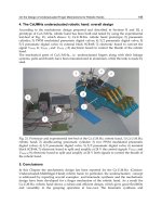
Our approach to integrate motion and deformation models is illustrated in Figure 1. In the
pre-computation process, as stated previously, the behavior of deformable objects in response
to impulsive forces is simulated using FEM program. Since the object is non-grounded or
ﬂoating in space, the impulsive force causes translational and rotational motion of the entire
body as well as deformation from its original shape. Our approach deals with the compo-
nents of motion and deformation separately. The component of deformation is represented by
IRDM; the component of motion is approximately retrieved by solving equations of motion,
hence there is no need of recording the component. In the interaction process, components
of motion and deformation are computed separately based on common interaction force and
then added together to obtain the resulting behavior.
Impulse
Response
Deformation
Model
Equation
of
Motion
original
deformed
and
moved
moved
deformed
Simulation

(Pre-Computation)
Presentation
(Reproduction)
Fig. 1. Integration of motion and deformation model
4.2 Process of pre-computation
As stated in section 4.1, objects motion consists of translation and rotation. Regarding trans-
lation, the motion of the center of gravity of the object is equal to the motion of point mass
that has identical mass with the object. Because of this equivalence, the translation of object is
obtained by computing the center of gravity at each time step.
ManipulationofDynamicallyDeformableObjectusingImpulse-BasedApproach 321
3.3 Interpolation of force on triangular patch
In the implementation of the algorithm that will be discussed in section 5, the proposed com-
putation method is adapted to models whose geometry is represented by triangular mesh.
Suppose the contact point p is found on a patch that has vertices p
1
, p
2
, and p
3
, and the in-
terface point is causing displacement u
p
. In our implementation, ﬁrstly, the reacting force in
the case when the displacement is caused on each of these vertex nodes. Such force is com-
puted using equation 8; we describe these forces as F
p
1
, F
p
2

, and F
p
3
. Next, by multiplying a
weighting factor to each of them, we determined the force applied to those nodes:
f
[t]
p
[t ]
1
= α
p
1
F
p
1
, f
[t]
p
[t ]
2
= α
p
2
F
p
2
, f
[t]
p

[t ]
3
= α
p
3
F
p
3
, (10)
where α
p
1
, α
p
2
, and α
p
3
are the area coordinates (or barycentric coordinate), and has relation-
ship as α
p
1
+ α
p
2
+ α
p
3
= 1. Using the result, the feedback force is computed as reaction of the
sum of the forces applied to the nodes:

F
p
= −( f
[t]
p
[t ]
1
+ f
[t]
p
[t ]
2
+ f
[t]
p
[t ]
3
). (11)
The result of this implementation when the interface point is interacting on a node is identical
with the result of equation 8. Also, the resulting feedback force is continuous on the boundary
of a triangular patch, or on edges and nodes.
Finally, the displacement on entire nodes of the model is computed by:
˜u
[t]
k
[t ]
=
T−1
∑
s=0

3
∑
i=1
R
[s]
p
[t −s]
i
k
[t ]
f
[t−s]
p
[t −s]
i
. (12)
3.4 Complexity of computation
Generally, computation of Equation 8 becomes easy if the number of ﬁxed DoF (i.e., DoF
with ﬁxed boundary condition) is small. In cases where DoF of a model is n and number of
ﬁxed DoF is n
c
, R
[0]
cc
becomes a n
c
× n
c
matrix. If the inverse of the matrix is computed using
simple Gauss elimination method, the order of the computation is O

(n
3
c
). On the other hand,
the order of computation cost of
˜
U
c
and
˜
U
o
are estimated to be O(n
2
c
· T) and O( n · n
c
· T)
respectively, considering that all of F
[t]
other than n
c
components is 0 for all past and present
time t.
Amount of memory that is required to store impulse response matrix is O
(n
2
· T), and O(n
c
·

T) to store past force boundary conditions.
4. Simulation of motion
Impulse response data of IRDM is obtained through simulation of deformation caused by
impulsive force. This process of precomputation causes problems in cases when the object is
not ﬁx on the ground. Interaction with non-grounded objects causes motion of the entire body
of the object that lasts for a long time, and representation of the motion of an entire body is
not suited for IRDM.
Let us think a method to deal with non-grounded deformable objects using IRDM. For exam-
ple, in a case where a deformable object is manipulated and pinched by the user, it becomes
unclear whether the displacement on the surface is derived from motion of object as a whole
or deformation of the object. It is impossible to represent the motion component that causes
permanent displacement using the IRDM model. Therefore, a computation method that sep-
arates these components apart and simulates motion and deformation is necessary.
In this section, a supplemental idea that realizes non-grounded motion of the deformable
model is presented.
As stated in section 3, the IRDM is based on the premise that the model is linear, however, in
a precise sense, motion and deformation of deformable object must be solved as a non-linear
coupled problem. For example, a spinning object is deformed by centrifugal force, the defor-
mation can cause change in an inertia moment, and the change affects the motion of rotation.
It is impossible to represent this non-linear coupled model using a linear model.
Fortunately, this non-linearity is not considered to be signiﬁcant in usual interaction using
hand, hence in our approach, it is assumed that motion and deformation can be separately
computed. Deformation and rigid motion of an object imposed by interaction force are com-
puted separately, and then the resulting behavior is obtained by adding then together. The
deformation and motion are simulated by using IRDM and solving equation of motion re-
spectively.
4.1 Separate simulation of motion and deformation
Our approach to integrate motion and deformation models is illustrated in Figure 1. In the
pre-computation process, as stated previously, the behavior of deformable objects in response
to impulsive forces is simulated using FEM program. Since the object is non-grounded or

ﬂoating in space, the impulsive force causes translational and rotational motion of the entire
body as well as deformation from its original shape. Our approach deals with the compo-
nents of motion and deformation separately. The component of deformation is represented by
IRDM; the component of motion is approximately retrieved by solving equations of motion,
hence there is no need of recording the component. In the interaction process, components
of motion and deformation are computed separately based on common interaction force and
then added together to obtain the resulting behavior.
Impulse
Response
Deformation
Model
Equation
of
Motion
original
deformed
and
moved
moved
deformed
Simulation
(Pre-Computation)
Presentation
(Reproduction)
Fig. 1. Integration of motion and deformation model
4.2 Process of pre-computation
As stated in section 4.1, objects motion consists of translation and rotation. Regarding trans-
lation, the motion of the center of gravity of the object is equal to the motion of point mass
that has identical mass with the object. Because of this equivalence, the translation of object is
obtained by computing the center of gravity at each time step.

AdvancesinHaptics322
Regarding the rotation of the object, an estimation algorithm based on geometric matching
was employed. The algorithm seeks rotation that minimizes the mean square error of node
positions when the deformed object is approximately represented by a non-deformed model.
The deformation component is obtained by subtracting the translational and rotational com-
ponent motion from the result of the simulation. By performing the process to all combina-
tions of DoF, the impulse response matrix R
[s]
is determined.
4.3 Process of presentation
As stated above, the deformation component and interaction force is computed using IRDM.
Then based on the interaction force, the component motion is computed by numerically solv-
ing initial-value problem of the motion equation (i.e., Newton’s and Euler’s equations):
m
dV
dt
=
∑
F
ext
(13)
ω
×(Iω) + I
dω
dt
=
∑
τ
ext
. (14)

where M is the mass of the entire body, I is inertia tensor, V and ω are velocity and angular
velocity of the rigid body respectively, and F
ext
and τ
ext
are external force and torque around
the center of gravity that are operated by the user. As stated above, in our approach, mutual
inﬂuence between rotation and deformation of the object is ignored. The computation cost of
IRDM is dominant in the total computation cost of this approach; hence the computational
advantage of IRDM is also inherited to this approach.
5. Experiment
This section describes experiments that evaluate feasibility and computation cost of deforma-
tion and interaction using IRDM.
5.1 Deformation
5.1.1 Pre-computation
Pre-computation is the process that computes impulse response data though deformation sim-
ulation; impulsive force is applied to each of all degrees of freedom and deformation response
on each of all degrees of freedom is recorded. Impulse response matrix R is obtained as a col-
lective of the data. Dynamic deformation of the model is simulated by using the FEM model
that consists of tetrahedral elements.
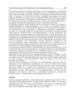
Three models of different complexity, as shown in Figure 2 were used for the evaluation: cat,
bunny, and cuboid; complexity of these models are summarized in Table 1. Fixed boundary
condition was applied to nodes on the bottom surface patches of the models; in order to ﬁx
the models to the ground. Height of the cat and bunny models is approximately 20cm, Height
and width of the cuboid model is 20cm and 10cm respectively. Physical parameters of all of
these models were deﬁned as: Young’s modulus E
= 2000N/m
2
, Poisson’s ratio ν = 0.49, and
density ρ

= 110kg/m
3
.
Impulse response was recorded for one second at a sampling rate of 500 Hz, hence each im-
pulse response wave in the impulse response matrix consists of 500 point sample values. Time
step of FEM simulation was changed accordingly to the velocity of object deformation from
0.1 to 2 ms. Computation time of FEM simulation that is required to obtain the entire impulse
response matrix for each model is shown in Table 1, where in house FEM routine by Pentium
4 3.0GHz processor was used.
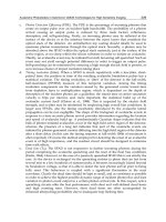
An example of impulse response of cuboid model is shown in Figure 3, where an impulsive
downward force has been applied on the node that is indicated by an arrow. Surface elastic
wave starts to diffuse from the node and propagate to entire body within approximately 16
ms.
(a) cat (b) bunny (c) cuboid
Fig. 2. Experimental models
cat bunny cuboid
free nodes (n) 359 826 1068
triangle patches 1796 3592 2178
entire nodes 690 1894 3312
tetrahedral elements 2421 8283 13310
pre-computation time (hr) 13.3 126.2 508.7
data size (GB) 4.3 22.8 38.2
Table 1. Complexity of models
5.1.2 Interaction
Experiments to evaluate interaction with models were carried out. Blockdiagram of the exper-
imental system is shown in Figure 4. The system consists of PC1 (CPU:Itanium2 1.4GHz
×4,
memory:32GB, OS:Linux) that is in charge of model computation, PC2 (CPU:Pentium3
500MHz
×2, OS:Windows) that serves as controller of two PHANToM devicesMassie (1996);

All computation related to the IRDM model is performed by PC1. Computation of force and
deformation are executed asynchronously using thread mechanism; these computations are
noted as force process and deformation process respectively in the rest of this paper.
In the force process, ﬁrstly interaction point information is received from the Ethernet inter-
face, next collision of the point with the surface of object model is detected, then interaction
force on the point is computed, history of interaction force is updated, and ﬁnally the interac-
tion force is output to the sent to PC2 through the Ethernet interface. Collision between the
interaction point and the object surface is computed using an algorithm that is similar to God-
Object MethodZilles & Salisbury (1995); this algorithm ﬁts with our implementation because
it eliminates ambiguity of the interaction point and provides unique displacement value. This
force process is repeatedly executed every 2 ms, or at a rate of 500 Hz.
Deformation process computes deformation of an object using the history of force computed
by the force process. As stated before, the impulse response matrix is a relatively large data
set, and the matrix must be held on the main memory while force and deformation processes
are executed. As suggested by Table 1, the data size of the cuboid model exceeds the size of
ManipulationofDynamicallyDeformableObjectusingImpulse-BasedApproach 323
Regarding the rotation of the object, an estimation algorithm based on geometric matching
was employed. The algorithm seeks rotation that minimizes the mean square error of node
positions when the deformed object is approximately represented by a non-deformed model.
The deformation component is obtained by subtracting the translational and rotational com-
ponent motion from the result of the simulation. By performing the process to all combina-
tions of DoF, the impulse response matrix R
[s]
is determined.
4.3 Process of presentation
As stated above, the deformation component and interaction force is computed using IRDM.
Then based on the interaction force, the component motion is computed by numerically solv-
ing initial-value problem of the motion equation (i.e., Newton’s and Euler’s equations):
m
dV

dt
=
∑
F
ext
(13)
ω
×(Iω) + I
dω
dt
=
∑
τ
ext
. (14)
where M is the mass of the entire body, I is inertia tensor, V and ω are velocity and angular
velocity of the rigid body respectively, and F
ext
and τ
ext
are external force and torque around
the center of gravity that are operated by the user. As stated above, in our approach, mutual
inﬂuence between rotation and deformation of the object is ignored. The computation cost of
IRDM is dominant in the total computation cost of this approach; hence the computational
advantage of IRDM is also inherited to this approach.
5. Experiment
This section describes experiments that evaluate feasibility and computation cost of deforma-
tion and interaction using IRDM.
5.1 Deformation
5.1.1 Pre-computation

Pre-computation is the process that computes impulse response data though deformation sim-
ulation; impulsive force is applied to each of all degrees of freedom and deformation response
on each of all degrees of freedom is recorded. Impulse response matrix R is obtained as a col-
lective of the data. Dynamic deformation of the model is simulated by using the FEM model
that consists of tetrahedral elements.
Three models of different complexity, as shown in Figure 2 were used for the evaluation: cat,
bunny, and cuboid; complexity of these models are summarized in Table 1. Fixed boundary
condition was applied to nodes on the bottom surface patches of the models; in order to ﬁx
the models to the ground. Height of the cat and bunny models is approximately 20cm, Height
and width of the cuboid model is 20cm and 10cm respectively. Physical parameters of all of
these models were deﬁned as: Young’s modulus E
= 2000N/m
2
, Poisson’s ratio ν = 0.49, and
density ρ
= 110kg/m
3
.
Impulse response was recorded for one second at a sampling rate of 500 Hz, hence each im-
pulse response wave in the impulse response matrix consists of 500 point sample values. Time
step of FEM simulation was changed accordingly to the velocity of object deformation from
0.1 to 2 ms. Computation time of FEM simulation that is required to obtain the entire impulse
response matrix for each model is shown in Table 1, where in house FEM routine by Pentium
4 3.0GHz processor was used.
An example of impulse response of cuboid model is shown in Figure 3, where an impulsive
downward force has been applied on the node that is indicated by an arrow. Surface elastic
wave starts to diffuse from the node and propagate to entire body within approximately 16
ms.
(a) cat (b) bunny (c) cuboid
Fig. 2. Experimental models

cat bunny cuboid
free nodes (n) 359 826 1068
triangle patches 1796 3592 2178
entire nodes 690 1894 3312
tetrahedral elements 2421 8283 13310
pre-computation time (hr) 13.3 126.2 508.7
data size (GB) 4.3 22.8 38.2
Table 1. Complexity of models
5.1.2 Interaction
Experiments to evaluate interaction with models were carried out. Blockdiagram of the exper-
imental system is shown in Figure 4. The system consists of PC1 (CPU:Itanium2 1.4GHz
×4,
memory:32GB, OS:Linux) that is in charge of model computation, PC2 (CPU:Pentium3
500MHz
×2, OS:Windows) that serves as controller of two PHANToM devicesMassie (1996);
All computation related to the IRDM model is performed by PC1. Computation of force and
deformation are executed asynchronously using thread mechanism; these computations are
noted as force process and deformation process respectively in the rest of this paper.
In the force process, ﬁrstly interaction point information is received from the Ethernet inter-
face, next collision of the point with the surface of object model is detected, then interaction
force on the point is computed, history of interaction force is updated, and ﬁnally the interac-
tion force is output to the sent to PC2 through the Ethernet interface. Collision between the
interaction point and the object surface is computed using an algorithm that is similar to God-
Object MethodZilles & Salisbury (1995); this algorithm ﬁts with our implementation because
it eliminates ambiguity of the interaction point and provides unique displacement value. This
force process is repeatedly executed every 2 ms, or at a rate of 500 Hz.
Deformation process computes deformation of an object using the history of force computed
by the force process. As stated before, the impulse response matrix is a relatively large data
set, and the matrix must be held on the main memory while force and deformation processes
are executed. As suggested by Table 1, the data size of the cuboid model exceeds the size of

AdvancesinHaptics324
t=0 t=2 t=4 t=6 t=8 t=16ms
t=24 t=32 t=40 t=48 t=56 t=64ms
Fig. 3. Examples of impulse response
main memory of PC1, hence only half of the data where interaction force is applied to nodes
on the upper half of the model were loaded on the main memory, and the area of interaction
by the user was limited to these upper half nodes.
Program of force and deformation processes running on PC1 was optimized by performance
using Intel Compiler and Performance Libraries. Deformation process was implemented us-
ing Math Kernel Library, parallelized by OpenMP Compiler, and three CPUs were allotted to
the computation.
PC2 serves as a local controller of the PHANToM device, it simply works as bidirectional
translator between the PHANToM device and Ethernet (TCP/IP) connection with PC1. Con-
trol of the device is implemented using GHOST library; control process of the library is exe-
cuted at 1kHz, and in the process, the latest data that is received from the Ethernet interface is
set to output force and the current position of interface point received from the device is sent
back to the Ethernet interface.
Ethernet
100BaseT
Force Proc.
Deformation
Proc.
Haptic
Update Proc.
OpenGL API
GHOST API
PC1 PC2
Fig. 4. System block diagram
5.1.3 Experimental Results
Figure 5 shows examples of interaction with a deformable object, where dynamic deformation

is presented by a sequence of images. Since it was impossible to store images in real time, these
images were generated off-line using the history of the interaction force; the arrow in the ﬁrst
image of each sequence indicates the point of application of force.
In ﬁgure 5(a), relatively quick motion of the cat model after releasing force that had been
applied on a node. Figures 5(b) and (c) show the vibration of the bunny model that is caused
by different interaction; the model was released after being pulled near and right in (b) and
(c) respectively. It should be noted that different a vibration mode is presented according to
different ways of interaction.
Figure 5(d) shows the deformation of cuboid model by step input of displacement; the force
is applied to a node that is identical with the node where impulse force was being applied in
Figure 3. Also, interaction force during the operation is plotted in Figure 6(a). Because of the
nature of the dynamic model, interaction force gradually approaches a balance point while
vibrating around the point.
Interaction using two interaction points is presented in Figure 5(e), where the user is pushing
on the left and right side of the face of the cat model. Interaction force during the operation
is plotted in Figure 6(b). As displacement on the right side increases, interaction force on the
left side is also increasing.
Finally, change of interaction force while the user traced the back of the cat model from neck
to tail is plotted in Figure 6(c). The plot suggests that interaction force is smoothly changing
all through the interaction. Although invisible from the plot, subtle vibration is felt during
contact with the object. The vibration is considered as an artifact that derives from sampling
rate of IRDM model, which is 500Hz in our current implementation. The vibration is thought
to be diminished by raising the sampling rate of the model in future implementation.
Evaluation of computation time is listed in Table 2. Computation of the interaction force
comprises the evaluation of 8 for 3 to 9 times. Overhead of collision detection, communication,
and graphic rendering is not included in values on the table. The computation of force is
sufﬁciently fast for haptic presentation in that it is performed within 0.5ms per cycle even in
case of using two interaction points.
Regarding deformation computation, real-time update of graphics at full video rate was not
attained. For example, in the case of the bunny model, the update rate deteriorated to approx-

imately 10 Hz. In spite of the low update rate, interaction was not felt greatly unreasonable
subjectively, probably because the interaction is depending on information of force that is
presented with less delay time.
cat bunny cuboid
Computation of interaction force
one-point 78 105 97
two-points 285 436 286
Computation of object deformation
one-point 13040 33578 42614
two-points 26451 67339 85705
Table 2. Computation time (µs)
ManipulationofDynamicallyDeformableObjectusingImpulse-BasedApproach 325
t=0 t=2 t=4 t=6 t=8 t=16ms
t=24 t=32 t=40 t=48 t=56 t=64ms
Fig. 3. Examples of impulse response
main memory of PC1, hence only half of the data where interaction force is applied to nodes
on the upper half of the model were loaded on the main memory, and the area of interaction
by the user was limited to these upper half nodes.
Program of force and deformation processes running on PC1 was optimized by performance
using Intel Compiler and Performance Libraries. Deformation process was implemented us-
ing Math Kernel Library, parallelized by OpenMP Compiler, and three CPUs were allotted to
the computation.
PC2 serves as a local controller of the PHANToM device, it simply works as bidirectional
translator between the PHANToM device and Ethernet (TCP/IP) connection with PC1. Con-
trol of the device is implemented using GHOST library; control process of the library is exe-
cuted at 1kHz, and in the process, the latest data that is received from the Ethernet interface is
set to output force and the current position of interface point received from the device is sent
back to the Ethernet interface.
Ethernet
100BaseT

Force Proc.
Deformation
Proc.
Haptic
Update Proc.
OpenGL API
GHOST API
PC1 PC2
Fig. 4. System block diagram
5.1.3 Experimental Results
Figure 5 shows examples of interaction with a deformable object, where dynamic deformation
is presented by a sequence of images. Since it was impossible to store images in real time, these
images were generated off-line using the history of the interaction force; the arrow in the ﬁrst
image of each sequence indicates the point of application of force.
In ﬁgure 5(a), relatively quick motion of the cat model after releasing force that had been
applied on a node. Figures 5(b) and (c) show the vibration of the bunny model that is caused
by different interaction; the model was released after being pulled near and right in (b) and
(c) respectively. It should be noted that different a vibration mode is presented according to
different ways of interaction.
Figure 5(d) shows the deformation of cuboid model by step input of displacement; the force
is applied to a node that is identical with the node where impulse force was being applied in
Figure 3. Also, interaction force during the operation is plotted in Figure 6(a). Because of the
nature of the dynamic model, interaction force gradually approaches a balance point while
vibrating around the point.
Interaction using two interaction points is presented in Figure 5(e), where the user is pushing
on the left and right side of the face of the cat model. Interaction force during the operation
is plotted in Figure 6(b). As displacement on the right side increases, interaction force on the
left side is also increasing.
Finally, change of interaction force while the user traced the back of the cat model from neck
to tail is plotted in Figure 6(c). The plot suggests that interaction force is smoothly changing

all through the interaction. Although invisible from the plot, subtle vibration is felt during
contact with the object. The vibration is considered as an artifact that derives from sampling
rate of IRDM model, which is 500Hz in our current implementation. The vibration is thought
to be diminished by raising the sampling rate of the model in future implementation.
Evaluation of computation time is listed in Table 2. Computation of the interaction force
comprises the evaluation of 8 for 3 to 9 times. Overhead of collision detection, communication,
and graphic rendering is not included in values on the table. The computation of force is
sufﬁciently fast for haptic presentation in that it is performed within 0.5ms per cycle even in
case of using two interaction points.
Regarding deformation computation, real-time update of graphics at full video rate was not
attained. For example, in the case of the bunny model, the update rate deteriorated to approx-
imately 10 Hz. In spite of the low update rate, interaction was not felt greatly unreasonable
subjectively, probably because the interaction is depending on information of force that is
presented with less delay time.
cat bunny cuboid
Computation of interaction force
one-point 78 105 97
two-points 285 436 286
Computation of object deformation
one-point 13040 33578 42614
two-points 26451 67339 85705
Table 2. Computation time (µs)
AdvancesinHaptics326
(a) t=0 t=60 t=120 t=180 t=240 t=300ms
(b) t=0 t=60 t=120 t=180 t=240 t=300ms
(c) t=0 t=60 t=120 t=180 t=240 t=300ms
(d) t=0 t=2 t=4 t=6 t=8 t=300ms
(e) scene 1 scene 2 (f) scene 3 scene 4
Fig. 5. Examples of dynamic deformation
5.2 Manipulation

5.2.1 Pre-computation
A cube model, 12cm on a side, as shown in Figure 7 was used for the evaluation; complexity of
the model is summarized in Table 3. Physical parameter of the model was deﬁned as: Young’s
modulus E
= 2000N/m
2
, Poisson’s ratio ν = 0.49, and density ρ = 110kg/m
3
.
The computation time of FEM simulation that is shown in Table 3, where commercial FEM
software (RADIOSS, Altair Engineering) with a Dual-Core Xeon 3.0GHz processor was used.
Components of solid body motion and deformation were separated using the algorithm de-
scribed in section 4 , and deformation component was stored as impulse response data.
Figure 8(a) shows that impulsive force is applied to the cube model; horizontal rightward force
on the ﬁgure has been applied. Since the cube is ﬂoating, it starts moving while causing similar
Time (s)
force (N)
(a)
right
left
(b)
Time (s)
force (N)
(c)
(scene 4)(scene 3)
0
1
0 0.1 0.2 0.3 0.4 0.5 0.6 0.7
(scene 1)
(scene 2)

force (N)
Time (s)
0
1
1 2 3 4 0
0
1
0 0.1 0.2 0.3 0.4 0.5 0.6 0.7
Fig. 6. Interaction force
deformation to the cuboid model. Figure 8(b) shows motion and deformation components
separately extracted from (a).
Fig. 7. Experimental model
5.2.2 Experimental Results
Figure 9 shows an example of a manipulating object; similarly to Figure 5, it presents se-
quences of images that were generated off-line.
In Figure 9(a), the user is picking up the top of a cube model and swinging right and left.
Interaction force and motion of center of gravity of the object during the operation is plotted
in Figure 10. The center of gravity motion is approximately sinusoidal, hence if the object is
rigid, interaction force is expected to show similar sinusoidal change. However, the actual
force is apparently causing oscillation at a different frequency. This fact suggests that the
object is vibrating at its natural vibration frequency.
ManipulationofDynamicallyDeformableObjectusingImpulse-BasedApproach 327
(a) t=0 t=60 t=120 t=180 t=240 t=300ms
(b) t=0 t=60 t=120 t=180 t=240 t=300ms
(c) t=0 t=60 t=120 t=180 t=240 t=300ms
(d) t=0 t=2 t=4 t=6 t=8 t=300ms
(e) scene 1 scene 2 (f) scene 3 scene 4
Fig. 5. Examples of dynamic deformation
5.2 Manipulation
5.2.1 Pre-computation

A cube model, 12cm on a side, as shown in Figure 7 was used for the evaluation; complexity of
the model is summarized in Table 3. Physical parameter of the model was deﬁned as: Young’s
modulus E
= 2000N/m
2
, Poisson’s ratio ν = 0.49, and density ρ = 110kg/m
3
.
The computation time of FEM simulation that is shown in Table 3, where commercial FEM
software (RADIOSS, Altair Engineering) with a Dual-Core Xeon 3.0GHz processor was used.
Components of solid body motion and deformation were separated using the algorithm de-
scribed in section 4 , and deformation component was stored as impulse response data.
Figure 8(a) shows that impulsive force is applied to the cube model; horizontal rightward force
on the ﬁgure has been applied. Since the cube is ﬂoating, it starts moving while causing similar
Time (s)
force (N)
(a)
right
left
(b)
Time (s)
force (N)
(c)
(scene 4)(scene 3)
0
1
0
0.1 0.2 0.3 0.4 0.5 0.6 0.7
(scene 1)
(scene 2)

force (N)
Time (s)
0
1
1 2 3 4 0
0
1
0
0.1 0.2 0.3 0.4 0.5 0.6 0.7
Fig. 6. Interaction force
deformation to the cuboid model. Figure 8(b) shows motion and deformation components
separately extracted from (a).
Fig. 7. Experimental model
5.2.2 Experimental Results
Figure 9 shows an example of a manipulating object; similarly to Figure 5, it presents se-
quences of images that were generated off-line.
In Figure 9(a), the user is picking up the top of a cube model and swinging right and left.
Interaction force and motion of center of gravity of the object during the operation is plotted
in Figure 10. The center of gravity motion is approximately sinusoidal, hence if the object is
rigid, interaction force is expected to show similar sinusoidal change. However, the actual
force is apparently causing oscillation at a different frequency. This fact suggests that the
object is vibrating at its natural vibration frequency.
AdvancesinHaptics328
free nodes (n) 866
triangle patches 1728
entire nodes 1360
tetrahedral elements 5309
pre-computation time per d.o.f. (s) 1462
data size per d.o.f. (MB) 9.9
Table 3. Complexity of model

(a) t=0 t=2 t=4 t=6 t=8 t=1000ms
(b) t=0 t=2 t=4 t=6 t=8 t=1000ms
Fig. 8. Example of impulse response
Figure 9(b) shows a case where the user is tapping on a node of the cube model. The effect of
both impact of collision and inertia of the object is reﬂected in the deformation and motion of
the object; also, similarly to interaction with grounded models, relatively quick deformation
is represented.
Figure 9(c) presents another example of interaction where the user is swirling the object along
an elliptic orbit whose lengths of major and minor axes were approximately 6cm and 3cm
respectively. Deformation that is caused by centrifugal force is represented naturally. Also, in
the author’s subjective impression, interaction force was realistic and reasonable.
6. Disucssion
6.1 Computation cost
As stated previously, computation complexity of the proposed method is independent of the
DoF of the entire model n and proportional to the DoF of ﬁxed boundary condition n
c
. Ex-
periments above have proved that, in cases when n
c
is small, it was possible to compute
interaction force in real time. Computation cost of deformation is O
(n
1
) and the feature of the
approach was also veriﬁed through experiments.
In cases of solving deformation by FEM, its computation cost depends on the algorithm of
the solver program. The order of the computation of simple Gauss elimination method is
O
(n
3

), and even in case of using iterative algorithm such as Gauss-Seidel method, the order
of computation is approximately O
(n
2
). This fact suggests that our approach is advantageous
as n becomes large.
Actually at present complexity of the model, the computation time that was required for pre-
computation process suggests that it is difﬁcult to perform the FEM simulation in real time,
(a) t=0 t=20 t=40 t=60 t=80 t=100ms
t=120 t=140 t=160 t=180 t=200 t=220ms
(b) t=0 t=4 t=8 t=100 t=400 t=800ms
(c) t=0 t=20 t=40 t=60 t=80 t=100ms
t=120 t=140 t=160 t=180 t=200 t=220ms
Fig. 9. Example of dynamic motion and deformation
-2
0
2
0
2
4
6
0 0.1 0.2 0.3 0.4 0.5 0.6 0.7 0.8
Time [s]
Displacement [cm] Force [N]
0.1 0.2 0.3 0.4 0.5 0.6 0.7 0.8
Time [s]
Left
Right
Fig. 10. Interaction force
although the FEM program that was employed for the computation was not aimed at real-time

simulation.
ManipulationofDynamicallyDeformableObjectusingImpulse-BasedApproach 329
free nodes (n) 866
triangle patches 1728
entire nodes 1360
tetrahedral elements 5309
pre-computation time per d.o.f. (s) 1462
data size per d.o.f. (MB) 9.9
Table 3. Complexity of model
(a) t=0 t=2 t=4 t=6 t=8 t=1000ms
(b) t=0 t=2 t=4 t=6 t=8 t=1000ms
Fig. 8. Example of impulse response
Figure 9(b) shows a case where the user is tapping on a node of the cube model. The effect of
both impact of collision and inertia of the object is reﬂected in the deformation and motion of
the object; also, similarly to interaction with grounded models, relatively quick deformation
is represented.
Figure 9(c) presents another example of interaction where the user is swirling the object along
an elliptic orbit whose lengths of major and minor axes were approximately 6cm and 3cm
respectively. Deformation that is caused by centrifugal force is represented naturally. Also, in
the author’s subjective impression, interaction force was realistic and reasonable.
6. Disucssion
6.1 Computation cost
As stated previously, computation complexity of the proposed method is independent of the
DoF of the entire model n and proportional to the DoF of ﬁxed boundary condition n
c
. Ex-
periments above have proved that, in cases when n
c
is small, it was possible to compute
interaction force in real time. Computation cost of deformation is O

(n
1
) and the feature of the
approach was also veriﬁed through experiments.
In cases of solving deformation by FEM, its computation cost depends on the algorithm of
the solver program. The order of the computation of simple Gauss elimination method is
O
(n
3
), and even in case of using iterative algorithm such as Gauss-Seidel method, the order
of computation is approximately O
(n
2
). This fact suggests that our approach is advantageous
as n becomes large.
Actually at present complexity of the model, the computation time that was required for pre-
computation process suggests that it is difﬁcult to perform the FEM simulation in real time,
(a) t=0 t=20 t=40 t=60 t=80 t=100ms
t=120 t=140 t=160 t=180 t=200 t=220ms
(b) t=0 t=4 t=8 t=100 t=400 t=800ms
(c) t=0 t=20 t=40 t=60 t=80 t=100ms
t=120 t=140 t=160 t=180 t=200 t=220ms
Fig. 9. Example of dynamic motion and deformation
-2
0
2
0
2
4
6

0 0.1 0.2 0.3 0.4 0.5 0.6 0.7 0.8
Time [s]
Displacement [cm] Force [N]
0.1 0.2 0.3 0.4 0.5 0.6 0.7 0.8
Time [s]
Left
Right
Fig. 10. Interaction force
although the FEM program that was employed for the computation was not aimed at real-time
simulation.
AdvancesinHaptics330
One idea to reduce deformation computation cost is approximately generating deformed
shape using reduced number of nodes; reduction of the number of nodes almost propor-
tionally reduces computation cost, and interpolation using curved surface contributes to pre-
sentation of smooth surface. Another idea is accelerating the computation process using an
advanced computing environment such as GPU. Our preliminary study is suggesting that the
computation of the IRDM model is well suited to parallel computation using GPU.
6.2 Memory consumption
Regarding memory consumption, IRDM of present implementation requires a relatively large
amount of memory and not applicable to practical application. Data compression method
to solve this problem has been investigated, and our preliminary experiment suggests that it
is possible to compress the data to approximately one-hundredth of original size by taking
advantage of similarities of impulse response waves related to nodes that are geometrically
close each other.
This compression method is expected to expand the area of application. For example, the size
of IRDM data of the cat model is approximately 4GB. Since the data must be held in main
memory during interaction, the computer that is available for the interaction is limited to
relatively high speciﬁcation machines. Also, the data size is somewhat too large to transmit
over the Internet. If the data is compressed to 40MB, it is easily handled using most current
computer systems and network connections.

6.3 Evaluation using subjects
Finally, evaluation of reality becomes an important topic of research, and as a basis for the
research, methodology to quantify reality of dynamic interaction with deformable object must
be established.
7. Conclusion
In this chapter, a novel approach to implement real-time interaction with deformable objects
was presented. A core idea of the approach is modeling deformation using a set of impulse
response data and computing deformation by convolution of interaction force with the model.
The idea was experimentally implemented and evaluated through experiments. Also, an ex-
tension of the model to represent non-grounded object is discussed, by which manipulation
of deformable object was enabled.
Finally, it should be noted that our approach is just one implementation of precomputation-
based deformation model. A model of this kind has problem of trade-off between number of
precomputed interaction and reality of presentation. The problem may be alleviated by intro-
ducing assumptions that effectively prevent combinational explosion of interaction patterns
and by compressing precomputed data based on similarity of response. Further investigation
is needed to ﬁnd better representation of precomputation-based models. We hope that this
paper will stimulate the discussion for such investigation.
8. References
B.Mirtich & J.Canny (1995). Impulse-based simulation of rigid bodies, Proc. Symp. Interactive
3D Graphics pp. 181–188.
Borst, C. & Indugula, A. (2005). Realistic virtual grasping, Proc. IEEE VR 2005 pp. 91–98.
D.Baraff (1989). Dynamic simulation of non-penetrating rigid bodies, Computer Graphics
23(3): 223–232.
G.Burdea (1996). Force and Touch Feedback for Virtual Reality, A Wiley-Inter-Science Publication,
New York.
GHOST SDK Programmer’s Guide (2002). SensAble Technologies, Inc.
Goeddeke, D., Strzodka, R. & Turek, S. (2005). Ergebnisberichte des instituts fur angewandte
mathematik, Nummer 292, FB Mathematik, Universitat Dortmund .
James, D. L. & Fatahalian, K. (2003). Precomputing interactive dynamic deformable scenes,

Proc. ACM SIGGRAPH 2003 pp. 879–887.
James, D. & Pai, D. (1999). Artdefo, accurate real time deformable objects.
J.E.Colgate, M.C.Stanley & J.M.Brown (1995). Issues in the haptic display of tool use, Proc.
IROS95 pp. 140–145.
K.Hirota & M.Hirose (2003). Dexterous object manipulation based on collision response, Proc.
IEEE VR 2003 pp. 232–239.
K.Hirota & T.Kaneko (2001). Haptic representation of elastic object.
K.Salisbury, D.Brock, T.Massie, N.Swarup & C.Zilles (1995). Haptic rendering: Programing
touch interaction with virtual objects, Proc. Symp. Interactive 3D Graphics pp. 123–130.
Kuchenbecker, K., Fiene, J. & Niemeyer, G. (2005). Event-based haptics and acceleration
matching: Portraying and assessing the realism of contact, Proc. WHC 2005 pp. 381–
387.
Massie, T. H. (1996). Initial Haptic Explorations with the Phantom: Virtual Touch Through Point
Interaction, Master Thiese at M.I.T.
Norton, A., Turk, G., Bacon, B., Gerth, J. & Sweeney, P. (1991). Animation of fracture by
physical modeling, Visual Computer 7: 210–219.
Okamura, A. M., Dennerlein, J. T. & Howe, R. D. (1998). Vibration feedback models for virtual
environments, Proc. IEEE ICRA pp. 2485–2490 (Vol.3).
Okamura, A. M., Hage, M. W., Cutkosky, M. R. & Dennerlein, J. T. (2000). Improving reality-
based models for vibration feedback, Proc. ASME DSCD DSC-Vol.69-2: 1117–1124.
Pai, D. K., van den Doel, K., James, D. L., Lang, J., Lloyd, J. E., Richmond, J. L. & Yau, S. H.
(2001). Scanning physical interaction behavior of 3d objects, Proc. ACM SIGGRAPH
2001 pp. 87–96.
Rohlf, J. & Helman, J. (1994). Iris performer: a high performance multiprocessing toolkit for
real-time 3d graphics, Proc. ACM SIGGRAPH 94 pp. 381–394.
S.Hasegawa & M.Sato (2004). Real-time rigid body simulation for haptic interactions based
on contact volume of polygonal objects, Computer Graphics Forum 23(3): 529–538.
Terzopoulos, D., Platt, J., Barr, A. & Fleischer, K. (1987). Elastically deformable models, Com-
puter Graphics 21(4): 205–214.
T.W.Sederberg & S.R.Parry (1986). Free-form deformation of solid geometric models, Computer

Graphics 20(4): 151–161.
T.Yoshikawa, Y.Yokokohji & nad X.Z.Zheng, T. (1995). Display of feel for the manipulation of
dynamic virtual objects, Trans. ASME J. DSMC 117(4): 554–558.
Wellman, P. & Howe, R. D. (1995). Towards realistic vibrotactile display in virtual environ-
ments, Proc. ASME DSCD DSC-Vol.57-2: 713–718.
Zilles, C. & Salisbury, K. (1995). A constraint-based god object method for haptic display, Proc.
IROS ’95 pp. 145–151.
ManipulationofDynamicallyDeformableObjectusingImpulse-BasedApproach 331
One idea to reduce deformation computation cost is approximately generating deformed
shape using reduced number of nodes; reduction of the number of nodes almost propor-
tionally reduces computation cost, and interpolation using curved surface contributes to pre-
sentation of smooth surface. Another idea is accelerating the computation process using an
advanced computing environment such as GPU. Our preliminary study is suggesting that the
computation of the IRDM model is well suited to parallel computation using GPU.
6.2 Memory consumption
Regarding memory consumption, IRDM of present implementation requires a relatively large
amount of memory and not applicable to practical application. Data compression method
to solve this problem has been investigated, and our preliminary experiment suggests that it
is possible to compress the data to approximately one-hundredth of original size by taking
advantage of similarities of impulse response waves related to nodes that are geometrically
close each other.
This compression method is expected to expand the area of application. For example, the size
of IRDM data of the cat model is approximately 4GB. Since the data must be held in main
memory during interaction, the computer that is available for the interaction is limited to
relatively high speciﬁcation machines. Also, the data size is somewhat too large to transmit
over the Internet. If the data is compressed to 40MB, it is easily handled using most current
computer systems and network connections.
6.3 Evaluation using subjects
Finally, evaluation of reality becomes an important topic of research, and as a basis for the
research, methodology to quantify reality of dynamic interaction with deformable object must

be established.
7. Conclusion
In this chapter, a novel approach to implement real-time interaction with deformable objects
was presented. A core idea of the approach is modeling deformation using a set of impulse
response data and computing deformation by convolution of interaction force with the model.
The idea was experimentally implemented and evaluated through experiments. Also, an ex-
tension of the model to represent non-grounded object is discussed, by which manipulation
of deformable object was enabled.
Finally, it should be noted that our approach is just one implementation of precomputation-
based deformation model. A model of this kind has problem of trade-off between number of
precomputed interaction and reality of presentation. The problem may be alleviated by intro-
ducing assumptions that effectively prevent combinational explosion of interaction patterns
and by compressing precomputed data based on similarity of response. Further investigation
is needed to ﬁnd better representation of precomputation-based models. We hope that this
paper will stimulate the discussion for such investigation.
8. References
B.Mirtich & J.Canny (1995). Impulse-based simulation of rigid bodies, Proc. Symp. Interactive
3D Graphics pp. 181–188.
Borst, C. & Indugula, A. (2005). Realistic virtual grasping, Proc. IEEE VR 2005 pp. 91–98.
D.Baraff (1989). Dynamic simulation of non-penetrating rigid bodies, Computer Graphics
23(3): 223–232.
G.Burdea (1996). Force and Touch Feedback for Virtual Reality, A Wiley-Inter-Science Publication,
New York.
GHOST SDK Programmer’s Guide (2002). SensAble Technologies, Inc.
Goeddeke, D., Strzodka, R. & Turek, S. (2005). Ergebnisberichte des instituts fur angewandte
mathematik, Nummer 292, FB Mathematik, Universitat Dortmund .
James, D. L. & Fatahalian, K. (2003). Precomputing interactive dynamic deformable scenes,
Proc. ACM SIGGRAPH 2003 pp. 879–887.
James, D. & Pai, D. (1999). Artdefo, accurate real time deformable objects.
J.E.Colgate, M.C.Stanley & J.M.Brown (1995). Issues in the haptic display of tool use, Proc.

IROS95 pp. 140–145.
K.Hirota & M.Hirose (2003). Dexterous object manipulation based on collision response, Proc.
IEEE VR 2003 pp. 232–239.
K.Hirota & T.Kaneko (2001). Haptic representation of elastic object.
K.Salisbury, D.Brock, T.Massie, N.Swarup & C.Zilles (1995). Haptic rendering: Programing
touch interaction with virtual objects, Proc. Symp. Interactive 3D Graphics pp. 123–130.
Kuchenbecker, K., Fiene, J. & Niemeyer, G. (2005). Event-based haptics and acceleration
matching: Portraying and assessing the realism of contact, Proc. WHC 2005 pp. 381–
387.
Massie, T. H. (1996). Initial Haptic Explorations with the Phantom: Virtual Touch Through Point
Interaction, Master Thiese at M.I.T.
Norton, A., Turk, G., Bacon, B., Gerth, J. & Sweeney, P. (1991). Animation of fracture by
physical modeling, Visual Computer 7: 210–219.
Okamura, A. M., Dennerlein, J. T. & Howe, R. D. (1998). Vibration feedback models for virtual
environments, Proc. IEEE ICRA pp. 2485–2490 (Vol.3).
Okamura, A. M., Hage, M. W., Cutkosky, M. R. & Dennerlein, J. T. (2000). Improving reality-
based models for vibration feedback, Proc. ASME DSCD DSC-Vol.69-2: 1117–1124.
Pai, D. K., van den Doel, K., James, D. L., Lang, J., Lloyd, J. E., Richmond, J. L. & Yau, S. H.
(2001). Scanning physical interaction behavior of 3d objects, Proc. ACM SIGGRAPH
2001 pp. 87–96.
Rohlf, J. & Helman, J. (1994). Iris performer: a high performance multiprocessing toolkit for
real-time 3d graphics, Proc. ACM SIGGRAPH 94 pp. 381–394.
S.Hasegawa & M.Sato (2004). Real-time rigid body simulation for haptic interactions based
on contact volume of polygonal objects, Computer Graphics Forum 23(3): 529–538.
Terzopoulos, D., Platt, J., Barr, A. & Fleischer, K. (1987). Elastically deformable models, Com-
puter Graphics 21(4): 205–214.
T.W.Sederberg & S.R.Parry (1986). Free-form deformation of solid geometric models, Computer
Graphics 20(4): 151–161.
T.Yoshikawa, Y.Yokokohji & nad X.Z.Zheng, T. (1995). Display of feel for the manipulation of
dynamic virtual objects, Trans. ASME J. DSMC 117(4): 554–558.

Wellman, P. & Howe, R. D. (1995). Towards realistic vibrotactile display in virtual environ-
ments, Proc. ASME DSCD DSC-Vol.57-2: 713–718.
Zilles, C. & Salisbury, K. (1995). A constraint-based god object method for haptic display, Proc.
IROS ’95 pp. 145–151.
AdvancesinHaptics332
HapticInteractionwithComplexModelsBasedonPrecomputations 333
HapticInteractionwithComplexModelsBasedonPrecomputations
IgorPeterlíkandLuděkMatyskaandJiříFilipovič
0
Haptic Interaction with Complex
Models Based on Precomputations
Igor Peterlík and Ludˇek Matyska and Ji ˇrí Filipoviˇc
Masaryk University
Czech Republic
1. Introduction
The real-time haptic interaction with deformable objects is an important area of research with
wide range of applications in medicine and industry. The development of computer-based
medical training systems (medical simulators) is perhaps the most challenging task, as it re-
quires physically-based modelling to mimic the behaviour of soft tissues. Such models are
usually based on the mathematical formulations emerging from the theory of elasticity, re-
sulting in non-linear boundary-value problems deﬁned over complex domains. Numerical
techniques such as the ﬁnite element method, which are needed to solve these problems, are
computationally expensive and therefore, their employment in the real-time interaction is not
straightforward, especially in haptics, where the refresh rate over 1 kHz is required.
There have been several approaches proposed so far to address the issue of coupling the heavy
computations with high refresh rate of the haptic loop. Basically, two main classes of solutions
can be identiﬁed: either simpliﬁed models based on linearization or reduction are used, or
some precomputation is employed before the real-time interaction takes place. In the ﬁrst
part of this chapter, an overview of the methods proposed in last decade is presented. Some
of them are described in detail to emphasize the key concepts which are used frequently in

haptic soft-tissue modeling nowadays.
In the second part of the chapter, an approach based on precomputation and interpolation
of precomputed data is presented. The technique consists of two procedures: ﬁrst, it is a
construction of a discrete set of data, which can be performed in reasonable time on today’s
computers. Second, it is a fast approximation of an arbitrary deformation which is needed
during the real-time interaction from the data constructed by the ﬁrst procedure.
In the text, both procedures are described conceptually emphasizing the computational as-
pect. An algorithm of distributed state-space search used for the precomputation procedure
is presented and then, three different types of the interpolations are studied and compared
w. r.t. the main features which are employed in the real-time interaction phase. After general
description, the evaluation of the method is brieﬂy given using a set of experiments being
done with a ﬁnite element 3D model of liver.
Finally, possibilities to couple the precomputation with interpolation, leading to a system ca-
pable of real-time interaction without off-line computations, is shortly discussed. The chapter
is concluded with summary of main features and advantages of the presented systems for
haptic interaction with complex models.
17
AdvancesinHaptics334
2. Methods for Haptic Rendering of Deformable Objects
2.1 Overview of Modelling Methods
The methods in the area of the deformation modelling can be ranged into two main groups
which are denoted as non-physical and physical. The non-physical methods are used mainly
in the computer graphics, as they are very fast and efﬁcient. Two well-known representatives
are spline modelling and free form deformations. In spline modelling, the curves and sur-
faces are represented by a set of control points and the shape of the objects is modiﬁed by
changing the position of the points. The main idea of free form deformations is to deform the
shape of the object by deforming the space in which the object is embedded. Generally, the
non-physical methods are not suitable in the case when the physically realistic behaviour of
the deformations is desired. In this case, the physical modeling is the only alternative.
The physical methods are based on the mathematical models usually formulated by partial-

differential equations (PDE). However, the main issue of this method is represented by the fact
that the resulting problem formulation is complex and the analytical solution is computation-
ally expensive or even infeasible. To address this issue, the models are simpliﬁed to cover the
essential observations and the equations are solved numerically. Bellow, the main methods
used in the physical modelling are presented with a brief description.
Mass-spring damper method (MSD). The mass is concentrated in a number of nodes which
are connected by springs, usually modelled as linear. When a force is applied to a node,
it starts to move and pass the force via springs to the neighbouring nodes. From the
computational point of view, the method is very simple and the cost of the calculation
is low. Although the method is based on physical model, the major drawback of MSD
systems is the insufﬁcient approximation of real material properties. They also suffer
from inaccuracy of the approximation in the case when the geometry of the object is
complex.
Finite difference method (FDM). The continuous derivative which appears in the PDE-
based formulations is replaced with a ﬁnite difference approximation, which is com-
puted in points organized in regular grid which spans over the domain of the object.
The technique is very accurate and efﬁcient for the objects with regular geometry. Nev-
ertheless, in case of complex shape of the domain, the discretization becomes extremely
dense, resulting in a huge computational complexity.
Boundary element method (BEM). The differential problem is converted to the integral
form, where under special conditions, the integration over the volumetric domain can
be substituted by the integration over its boundary. The models based on this model
cannot cope with any phenomena related to the volume of the body because of the re-
duction presented above, so e.g. the applied volume forces or heterogeneity of the body
cannot be considered.
Finite element method (FEM). Finite elements are widely used for modelling of soft tissues,
since they are directly based on the theory of the elasticity and provide very good ap-
proximation for the complex geometries. The method generally consists of discretiza-
tion of the domain and mathematical re-formulation of the boundary-value problem
resulting in large systems of algebraic equations. The ﬁnite element method seems to

be superior to the other methods when the modelling complex bodies with non-trivial
physical properties is considered. It is also suitable when volumetric operations such
as cutting and tearing are to be modelled, as the entire domain of the body is included
in the formulation.
(a) (b)
Fig. 1. Deformations of FE mesh of human liver (rest position depicted in gray) for (a) linear
elasticity model, (b) non-linear Mooney-Rivlin model with complete strain tensor. In both
cases, the same force was applied to a node in the left part of the body.
In the following text, we focus on the methods which are based on the physical approach.
More precisely, the ﬁnite element (FE) models are brieﬂy introduced and the most important
methods employing the real-time haptic interaction are surveyed.
2.2 Overview of FE models
The physically based deformation modeling is based on relation derived within the frame of
elasticity theory. A detailed description of the mathematical formulation can be found for ex-
ample in Ciarlet (1988); J.T.Oden (1972); Wriggers (2008). The realistic behaviour of the objects
modelled by the ﬁnite element method is usually validated w. r. t. the real measurements. In
the following text, only some basic terms are informally introduced in order to identify the
main issues which are associated with real-time haptic modeling of soft tissues.
When speaking about the modeling of deformations, two types of non-linearities are usually
considered. First, the geometric non-linearity introduces non-linear relation between the dis-
placement and strain. In case when the non-linear term in the deﬁnition of the strain tensor
is neglected, only small deformations are rendered correctly. For larger deformations, the vol-
ume of the deformable object is not preserved and the overall behaviour of the object is not
realistic. Therefore, geometrically non-linear model must be used when large deformations
take place. The difference in behavior between geometrically linear and non-linear model is
demonstrated in Fig. 1.
Second, physical non-linearity is introduced if non-linear relation between the stress and
strain is used. The visual difference between physically linear and non-linear model is not
so apparent, nevertheless, this type of non-linearity heavily affects the force response of the
body and it plays an important role for realistic simulation of the soft tissues (see Misra et al.

(2007)). Physically non-linear model is represented by Mooney-Rivlin material employing the
non-linear incompressibility condition.
Putting it all together, both non-linearities are of a great importance when realistic modelling
is required, since the geometrically linear model cannot handle large deformations properly,
whereas physically linear model is limiting w. r. t. the material properties. Nevertheless, both
geometrically and physically linear models have been extensively used in the past because of
HapticInteractionwithComplexModelsBasedonPrecomputations 335
2. Methods for Haptic Rendering of Deformable Objects
2.1 Overview of Modelling Methods
The methods in the area of the deformation modelling can be ranged into two main groups
which are denoted as non-physical and physical. The non-physical methods are used mainly
in the computer graphics, as they are very fast and efﬁcient. Two well-known representatives
are spline modelling and free form deformations. In spline modelling, the curves and sur-
faces are represented by a set of control points and the shape of the objects is modiﬁed by
changing the position of the points. The main idea of free form deformations is to deform the
shape of the object by deforming the space in which the object is embedded. Generally, the
non-physical methods are not suitable in the case when the physically realistic behaviour of
the deformations is desired. In this case, the physical modeling is the only alternative.
The physical methods are based on the mathematical models usually formulated by partial-
differential equations (PDE). However, the main issue of this method is represented by the fact
that the resulting problem formulation is complex and the analytical solution is computation-
ally expensive or even infeasible. To address this issue, the models are simpliﬁed to cover the
essential observations and the equations are solved numerically. Bellow, the main methods
used in the physical modelling are presented with a brief description.
Mass-spring damper method (MSD). The mass is concentrated in a number of nodes which
are connected by springs, usually modelled as linear. When a force is applied to a node,
it starts to move and pass the force via springs to the neighbouring nodes. From the
computational point of view, the method is very simple and the cost of the calculation
is low. Although the method is based on physical model, the major drawback of MSD
systems is the insufﬁcient approximation of real material properties. They also suffer

from inaccuracy of the approximation in the case when the geometry of the object is
complex.
Finite difference method (FDM). The continuous derivative which appears in the PDE-
based formulations is replaced with a ﬁnite difference approximation, which is com-
puted in points organized in regular grid which spans over the domain of the object.
The technique is very accurate and efﬁcient for the objects with regular geometry. Nev-
ertheless, in case of complex shape of the domain, the discretization becomes extremely
dense, resulting in a huge computational complexity.
Boundary element method (BEM). The differential problem is converted to the integral
form, where under special conditions, the integration over the volumetric domain can
be substituted by the integration over its boundary. The models based on this model
cannot cope with any phenomena related to the volume of the body because of the re-
duction presented above, so e.g. the applied volume forces or heterogeneity of the body
cannot be considered.
Finite element method (FEM). Finite elements are widely used for modelling of soft tissues,
since they are directly based on the theory of the elasticity and provide very good ap-
proximation for the complex geometries. The method generally consists of discretiza-
tion of the domain and mathematical re-formulation of the boundary-value problem
resulting in large systems of algebraic equations. The ﬁnite element method seems to
be superior to the other methods when the modelling complex bodies with non-trivial
physical properties is considered. It is also suitable when volumetric operations such
as cutting and tearing are to be modelled, as the entire domain of the body is included
in the formulation.
(a) (b)
Fig. 1. Deformations of FE mesh of human liver (rest position depicted in gray) for (a) linear
elasticity model, (b) non-linear Mooney-Rivlin model with complete strain tensor. In both
cases, the same force was applied to a node in the left part of the body.
In the following text, we focus on the methods which are based on the physical approach.
More precisely, the ﬁnite element (FE) models are brieﬂy introduced and the most important
methods employing the real-time haptic interaction are surveyed.

2.2 Overview of FE models
The physically based deformation modeling is based on relation derived within the frame of
elasticity theory. A detailed description of the mathematical formulation can be found for ex-
ample in Ciarlet (1988); J.T.Oden (1972); Wriggers (2008). The realistic behaviour of the objects
modelled by the ﬁnite element method is usually validated w. r. t. the real measurements. In
the following text, only some basic terms are informally introduced in order to identify the
main issues which are associated with real-time haptic modeling of soft tissues.
When speaking about the modeling of deformations, two types of non-linearities are usually
considered. First, the geometric non-linearity introduces non-linear relation between the dis-
placement and strain. In case when the non-linear term in the deﬁnition of the strain tensor
is neglected, only small deformations are rendered correctly. For larger deformations, the vol-
ume of the deformable object is not preserved and the overall behaviour of the object is not
realistic. Therefore, geometrically non-linear model must be used when large deformations
take place. The difference in behavior between geometrically linear and non-linear model is
demonstrated in Fig. 1.
Second, physical non-linearity is introduced if non-linear relation between the stress and
strain is used. The visual difference between physically linear and non-linear model is not
so apparent, nevertheless, this type of non-linearity heavily affects the force response of the
body and it plays an important role for realistic simulation of the soft tissues (see Misra et al.
(2007)). Physically non-linear model is represented by Mooney-Rivlin material employing the
non-linear incompressibility condition.
Putting it all together, both non-linearities are of a great importance when realistic modelling
is required, since the geometrically linear model cannot handle large deformations properly,
whereas physically linear model is limiting w. r. t. the material properties. Nevertheless, both
geometrically and physically linear models have been extensively used in the past because of

Advances in Haptics Part 9 docx

Tài liệu liên quan

Tài liệu bạn tìm kiếm đã sẵn sàng tải về