Advances in Measurement Systems Part 2 pdf

Bạn đang xem bản rút gọn của tài liệu. Xem và tải ngay bản đầy đủ của tài liệu tại đây (7.46 MB, 40 trang )

AdvancesinMeasurementSystems36
Zhang & Huang (2006b) proposed a new structured light system calibration method. In
this method, the fringe images are used as a tool to establish the mapping between the
camera pixel and the projector pixel so that the projector can “capture" images like a
camera. By this means, the structured light system calibration becomes a well studied
stereo system calibration. Since the projector and the camera are calibrated independently
and simultaneously, the calibration accuracy is signiﬁcantly improved, and the calibration
speed is drastically increased. Fig. 4 shows a typical checkerboard image pair captured
by the camera, and the projector image converted by the mapping method. It clearly
shows that the projector checkerboard image is well captured. By capturing a number
of checkerboard image pairs and applying the software algorithm developed by Bouguet
( both the camera and the projector are
calibrated at the same time.
(a) (b)
Fig. 4. Checkerboard image pair by using the proposed technique by Zhang and
Huang (Zhang & Huang, 2006b). (a) The checkerboard image captured by the camera; (b)
The mapped checkerboard image for the projector, which is regarded as the checkerboard
image captured by the projector.
Following thework byZhang &Huang (2006b), a number of calibration approaches have been
developed (Gao et al., 2008; Huang & Han, 2006; Li et al., 2008; Yang et al., 2008). All these
techniques are essentially the same: to establish the one-to-one mapping between the projector
and the camera. Our recent work showed that the checker size of the checkerboard plays a
key role (Lohry et al., 2009), and a certain range of checker size will give better calibration
accuracy. This study provides some guidelines for selecting the checker size for precise system
calibration. Once the system is calibrated, the xyz coordinates can be computed from the
absolute phase, which will be addressed in the next subsection.
2.7 3-D coordinate calculation from the absolute phase
Once the absolute phase map is obtained, the relationship between the camera sensor and
projector sensor will be established as a one-to-many mapping, i.e., one point on the camera
sensor corresponds to one line on the projector sensor with the same absolute phase value.

This relationship provides a constraint for the correspondence of a camera-projector system.
If the camera and the projector are calibrated in the same world coordinate system, and the
linear calibration model is used for both the camera and the projector, Eq. (11) can be re-written
as
s
c
I
c
= A
c
[
R
c
, t
c
]X
w
. (12)
Here, s
c
is the scaling factor for the camera, I
c
the homogeneous camera image coordinates,
A
c
the intrinsic parameters for the camera, and [R
c
, t
c
] the extrinsic parameter matrix for the

camera.
Similarly, the relationship between the projector image point and the object point in the world
coordinate system can be written as
s
p
I
p
= A
p
[
R
p
, t
p
]X
w
. (13)
Here s
p
is the scaling factor for the projector, I
p
the homogeneous projector image coordinates,
A
p
the intrinsic parameters for the projector, [R
p
, t
p
] the extrinsic parameter matrix for the
projector.

In addition, because absolute phase is known, each point on the camera corresponds to one
line with the same absolute phase on the projected fringe image (Zhang & Huang, 2006b).
That is, assume the fringe stripe is along v direction, we can establish a relationship between
the captured fringe image and the projected fringe image,
φ
a
(u
c
, v
c
) = φ
a
(u
p
). (14)
In Equations (12)-(14), there are seven unknowns
(x
w
, y
w
, z
w
), s
p
, s
p
, u
p
, and v
p

, and seven
equations, the world coordinates
(x
w
, y
w
, z
w
) can be uniquely solved for.
2.8 Example of measurement
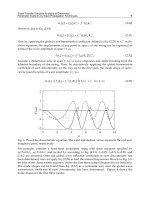
Fig. 5 shows an example of 3-D shape measurement using a three-step phase-shifting method.
Fig. 5(a)-5(c) shows three phase-shifted fringe images with 2π/3 phase shift. Fig. 5(d) shows
the phase map after applying Eq. (4) to these fringe images, it clearly shows phase discon-
tinuities. Applying the phase unwrapping algorithm discussed in Reference (Zhang et al.,
2007), this wrapped phase map can be unwrapped to get a continuous phase map as shown
in Fig. 5(e). The unwrapped phase map is then converted to 3-D shape by applying method in-
troduced in Section 2.7. The 3-D shape can be rendered by OpenGL, as shown in Figs. 5(f)-5(g).
At the same time, by averaging these three fringe images, a texture image can be obtained,
which can be mapped onto the 3-D shape to for better visual effect, as seen in Fig. 5(h).
3. Real-time 3-D Shape Measurement Techniques
3.1 Hardware implementation of phase-shifting technique for real-time data acquisition
From Section 2, we know that, for a three-step phase-shifting algorithm, only three images
are required to reconstruct one 3-D shape. This, therefore, permits the possibility of encoding
them into a single color image. As explained in Section 2, using color fringe pattern is not
desirable for 3-D shape measurement because of the problems caused by color. To avoid this
problem, we developed a real-time 3-D shape measurement system based on a single-chip
DLP projection and white light technique (Zhang & Huang, 2006a).
Fig. 6 shows the system layout. Three phase-shifted fringe images are encoded with the RGB
color channel of a color fringe image generated by the computer. The color image is then
sent to the single-chip DLP projector that switches three-color channels sequentially onto the

object; a high-speed CCD camera, synchronized with the projector, is to capture three phase-
shifted fringe images at high speed. Any three fringe images can be used to reconstruct one
High-resolution,High-speed3-DDynamicallyDeformable
ShapeMeasurementUsingDigitalFringeProjectionTechniques 37
Zhang & Huang (2006b) proposed a new structured light system calibration method. In
this method, the fringe images are used as a tool to establish the mapping between the
camera pixel and the projector pixel so that the projector can “capture" images like a
camera. By this means, the structured light system calibration becomes a well studied
stereo system calibration. Since the projector and the camera are calibrated independently
and simultaneously, the calibration accuracy is signiﬁcantly improved, and the calibration
speed is drastically increased. Fig. 4 shows a typical checkerboard image pair captured
by the camera, and the projector image converted by the mapping method. It clearly
shows that the projector checkerboard image is well captured. By capturing a number
of checkerboard image pairs and applying the software algorithm developed by Bouguet
( both the camera and the projector are
calibrated at the same time.
(a) (b)
Fig. 4. Checkerboard image pair by using the proposed technique by Zhang and
Huang (Zhang & Huang, 2006b). (a) The checkerboard image captured by the camera; (b)
The mapped checkerboard image for the projector, which is regarded as the checkerboard
image captured by the projector.
Following the work by Zhang & Huang (2006b), a number of calibration approaches have been
developed (Gao et al., 2008; Huang & Han, 2006; Li et al., 2008; Yang et al., 2008). All these
techniques are essentially the same: to establish the one-to-one mapping between the projector
and the camera. Our recent work showed that the checker size of the checkerboard plays a
key role (Lohry et al., 2009), and a certain range of checker size will give better calibration
accuracy. This study provides some guidelines for selecting the checker size for precise system
calibration. Once the system is calibrated, the xyz coordinates can be computed from the
absolute phase, which will be addressed in the next subsection.
2.7 3-D coordinate calculation from the absolute phase

Once the absolute phase map is obtained, the relationship between the camera sensor and
projector sensor will be established as a one-to-many mapping, i.e., one point on the camera
sensor corresponds to one line on the projector sensor with the same absolute phase value.
This relationship provides a constraint for the correspondence of a camera-projector system.
If the camera and the projector are calibrated in the same world coordinate system, and the
linear calibration model is used for both the camera and the projector, Eq. (11) can be re-written
as
s
c
I
c
= A
c
[
R
c
, t
c
]X
w
. (12)
Here, s
c
is the scaling factor for the camera, I
c
the homogeneous camera image coordinates,
A
c
the intrinsic parameters for the camera, and [R
c

, t
c
] the extrinsic parameter matrix for the
camera.
Similarly, the relationship between the projector image point and the object point in the world
coordinate system can be written as
s
p
I
p
= A
p
[
R
p
, t
p
]X
w
. (13)
Here s
p
is the scaling factor for the projector, I
p
the homogeneous projector image coordinates,
A
p
the intrinsic parameters for the projector, [R
p
, t

p
] the extrinsic parameter matrix for the
projector.
In addition, because absolute phase is known, each point on the camera corresponds to one
line with the same absolute phase on the projected fringe image (Zhang & Huang, 2006b).
That is, assume the fringe stripe is along v direction, we can establish a relationship between
the captured fringe image and the projected fringe image,
φ
a
(u
c
, v
c
) = φ
a
(u
p
). (14)
In Equations (12)-(14), there are seven unknowns
(x
w
, y
w
, z
w
), s
p
, s
p
, u

p
, and v
p
, and seven
equations, the world coordinates
(x
w
, y
w
, z
w
) can be uniquely solved for.
2.8 Example of measurement
Fig. 5 shows an example of 3-D shape measurement using a three-step phase-shifting method.
Fig. 5(a)-5(c) shows three phase-shifted fringe images with 2π/3 phase shift. Fig. 5(d) shows
the phase map after applying Eq. (4) to these fringe images, it clearly shows phase discon-
tinuities. Applying the phase unwrapping algorithm discussed in Reference (Zhang et al.,
2007), this wrapped phase map can be unwrapped to get a continuous phase map as shown
in Fig. 5(e). The unwrapped phase map is then converted to 3-D shape by applying method in-
troduced in Section 2.7. The 3-D shape can be rendered by OpenGL, as shown in Figs. 5(f)-5(g).
At the same time, by averaging these three fringe images, a texture image can be obtained,
which can be mapped onto the 3-D shape to for better visual effect, as seen in Fig. 5(h).
3. Real-time 3-D Shape Measurement Techniques
3.1 Hardware implementation of phase-shifting technique for real-time data acquisition
From Section 2, we know that, for a three-step phase-shifting algorithm, only three images
are required to reconstruct one 3-D shape. This, therefore, permits the possibility of encoding
them into a single color image. As explained in Section 2, using color fringe pattern is not
desirable for 3-D shape measurement because of the problems caused by color. To avoid this
problem, we developed a real-time 3-D shape measurement system based on a single-chip
DLP projection and white light technique (Zhang & Huang, 2006a).

Fig. 6 shows the system layout. Three phase-shifted fringe images are encoded with the RGB
color channel of a color fringe image generated by the computer. The color image is then
sent to the single-chip DLP projector that switches three-color channels sequentially onto the
object; a high-speed CCD camera, synchronized with the projector, is to capture three phase-
shifted fringe images at high speed. Any three fringe images can be used to reconstruct one
AdvancesinMeasurementSystems38
(a) (b) (c) (d)
(e) (f) (g) (h)
Fig. 5. . Example of 3-D shape measurement using a three-step phase-shifting method. (a)
I
1
(−2π/3); (b) I
2
(0); (c) I
3
(2π/3); (d) Wrapped phase map; (e) Unwrapped phase map; (f)
3-D shape rendered in shaded mode; (g) Zoom in view; (h) 3-D shape rendered with texture
mapping.
3-D shape through phase wrapping and unwrapping. Moreover, by averaging these three
fringe images, a texture image (without fringe stripes) can be generated. It can be used for
texture mapping purposed to enhance certain view effect.
The projector projects a monochrome fringe image for each of the RGB channels sequentially;
the color is a result of a color wheel placed in front of a projection lens. Each “frame" of the
projected image is actually three separate images. By removing the color wheel and placing
each fringe image in a separate channel, the projector can produce three fringe images at 120
fps (360 individual fps). Therefore, if three fringe images are sufﬁcient to recover one 3-D
shape, the 3-D measurement speed is up to 120 Hz. However, due to the speed limit of the
camera used, it takes two projection cycles to capture three fringe images, thus the measure-
ment speed is 60 Hz. Fig. 7 shows the timing chart for the real-time 3-D shape measurement
system.

3.2 Fast phase-shifting algorithm
The hardware system described in previous subsection can acquire fringe images at 180 Hz.
However, the processing speed needs to keep up with the data acquisition for real-time 3-
D shape measurement. The ﬁrst challenge is to increase the processing speed of the phase
Object
Projector
fringe
Camera
image
Phase line
Projector
pixel
Camera
pixel
Object
point
Phase line
Baseline
C A
B
E
D
Z
DLP
projector
RGB
fringe
Object
PC
CCD

camera
R
G
B
Wrapped
phase map
3D W/
Texture
I
1
I
2
I
3
3D
model
2D
photo
Fig. 6. Real-time 3-D shape measurement system layout. The computer generated color en-
coded fringe image is sent to a single-chip DLP projector that projects three color channels
sequentially and repeatedly in grayscale onto the object. The camera, precisely synchronized
with projector, is used to capture three individual channels separately and quickly. By apply-
ing the three-step phase-shifting algorithm to three fringe images, the 3-D geometry can be
recovered. Averaging three fringe images will result in a texture image that can be further
mapped onto 3-D shape to enhance certain visual effect.
wrapping. Experiments found that calculating the phase using Eq. (4) is relatively slow for
the purpose of real-time 3-D shape measurement. To improve the processing speed, Huang
et al. (2005) developed a new algorithm named trapezoidal phase-shifting algorithm. The
advantage of this algorithm is that it processes the phase by intensity ratio instead of arct-
angent function, thus signiﬁcantly improves the processing speed (more than 4 times faster).

However, the drawback of this algorithm is that the defocusing of the system will introduce
error, albeit to a less degree. This is certainly not desirable. Because the sinusoidal fringe
patterns are not very sensitive to defocusing problems, we applied the same processing algo-
rithm to sinusoidal fringe, the purpose is to maintain the advantage of processing speed while
alleviate the defocusing problem, this new algorithm is called fast three-step phase-shifting al-
gorithm (Huang & Zhang, 2006).
Fig. 8 illustrates this fast three-step phase-shifting algorithm. Instead of calculating phase
using an arctangent function, the phase is approximated by intensity ratio
r
(x, y) =
I
med
(x, y) − I
min
(x, y)
I
max
(x, y) − I
min
(x, y)
. (15)
Here I
max
, I
med
, I
min
respectively refer to the maximum, median, and minimum intensity value
for three fringe images for the same point. The intensity ratio gives values ranging from [0,
High-resolution,High-speed3-DDynamicallyDeformable

ShapeMeasurementUsingDigitalFringeProjectionTechniques 39
(a) (b) (c) (d)
(e) (f) (g) (h)
Fig. 5. . Example of 3-D shape measurement using a three-step phase-shifting method. (a)
I
1
(−2π/3); (b) I
2
(0); (c) I
3
(2π/3); (d) Wrapped phase map; (e) Unwrapped phase map; (f)
3-D shape rendered in shaded mode; (g) Zoom in view; (h) 3-D shape rendered with texture
mapping.
3-D shape through phase wrapping and unwrapping. Moreover, by averaging these three
fringe images, a texture image (without fringe stripes) can be generated. It can be used for
texture mapping purposed to enhance certain view effect.
The projector projects a monochrome fringe image for each of the RGB channels sequentially;
the color is a result of a color wheel placed in front of a projection lens. Each “frame" of the
projected image is actually three separate images. By removing the color wheel and placing
each fringe image in a separate channel, the projector can produce three fringe images at 120
fps (360 individual fps). Therefore, if three fringe images are sufﬁcient to recover one 3-D
shape, the 3-D measurement speed is up to 120 Hz. However, due to the speed limit of the
camera used, it takes two projection cycles to capture three fringe images, thus the measure-
ment speed is 60 Hz. Fig. 7 shows the timing chart for the real-time 3-D shape measurement
system.
3.2 Fast phase-shifting algorithm
The hardware system described in previous subsection can acquire fringe images at 180 Hz.
However, the processing speed needs to keep up with the data acquisition for real-time 3-
D shape measurement. The ﬁrst challenge is to increase the processing speed of the phase
Object

Projector
fringe
Camera
image
Phase line
Projector
pixel
Camera
pixel
Object
point
Phase line
Baseline
C A
B
E
D
Z
DLP
projector
RGB
fringe
Object
PC
CCD
camera
R
G
B
Wrapped

phase map
3D W/
Texture
I
1
I
2
I
3
3D
model
2D
photo
Fig. 6. Real-time 3-D shape measurement system layout. The computer generated color en-
coded fringe image is sent to a single-chip DLP projector that projects three color channels
sequentially and repeatedly in grayscale onto the object. The camera, precisely synchronized
with projector, is used to capture three individual channels separately and quickly. By apply-
ing the three-step phase-shifting algorithm to three fringe images, the 3-D geometry can be
recovered. Averaging three fringe images will result in a texture image that can be further
mapped onto 3-D shape to enhance certain visual effect.
wrapping. Experiments found that calculating the phase using Eq. (4) is relatively slow for
the purpose of real-time 3-D shape measurement. To improve the processing speed, Huang
et al. (2005) developed a new algorithm named trapezoidal phase-shifting algorithm. The
advantage of this algorithm is that it processes the phase by intensity ratio instead of arct-
angent function, thus signiﬁcantly improves the processing speed (more than 4 times faster).
However, the drawback of this algorithm is that the defocusing of the system will introduce
error, albeit to a less degree. This is certainly not desirable. Because the sinusoidal fringe
patterns are not very sensitive to defocusing problems, we applied the same processing algo-
rithm to sinusoidal fringe, the purpose is to maintain the advantage of processing speed while
alleviate the defocusing problem, this new algorithm is called fast three-step phase-shifting al-

gorithm (Huang & Zhang, 2006).
Fig. 8 illustrates this fast three-step phase-shifting algorithm. Instead of calculating phase
using an arctangent function, the phase is approximated by intensity ratio
r
(x, y) =
I
med
(x, y) − I
min
(x, y)
I
max
(x, y) − I
min
(x, y)
. (15)
Here I
max
, I
med
, I
min
respectively refer to the maximum, median, and minimum intensity value
for three fringe images for the same point. The intensity ratio gives values ranging from [0,
AdvancesinMeasurementSystems40
R G B R G B R G B
Projector signal
Camera signal
Exp. GExp. R Exp. B Exp. R Exp. B
Projection period

t = 1/120 sec
Acquisition time
t = 1/60 sec
Fig. 7. System timing chart.
),( yx

3/
T
3/2
T
6/5
T
),( yxs
0
6/
T
0
6
1

N
2
3
4
5
6
2/
T
T
(c)

(b)
),( yx

3/
T
3/2
T
6/5
T
),( y
x
r
0
6/
T
0
1
1

N
2
3
4
5
6
2/
T
T
),( yx


3/
T
3/2
T
6/5
T
0
6/
T
0
1

N
2
3
4
5
6
2/
T
T
(d)
),( yx

),( yxI
1

N
2
3

4
5
6
),(' y
x
I
),(" y
x
I
3/2

0
3/


3/4

3/5


2
(a)
),( yx


2
Fig. 8. Schematic illustration for fast three-step phase-shifting algorithm. (a) One period of
fringe is uniformly divided into six regions; (b) The intensity ratio for one period of fringe; (c)
After slope map after removing the sawtooth shape of the intensity ratio map; (d) The phase
after compensate for the approximation error and scaled to its original phase value.

1] periodically within one period of the fringe pattern. Fig. 8(a) shows that one period of the
fringe pattern is uniformly divided into six regions. It is interesting to know that the region
number N can be uniquely identiﬁed by comparing the intensity values of three fringe images
point by point. For example, if red is the largest, and blue is the smallest, the point belongs
to region N
= 1. Once the region number is identiﬁed, the sawtooth shape intensity ratio in
Fig. 8(b) can be converted to its slope shape in Fig. 8(c) by using the following equation
s
(x, y) = 2 × Floor

N
2

+ (−1)
N−1
r(x, y). (16)
Here the operator Floor
() is used to truncate the ﬂoating point data to keep the integer part
only. The phase can then be computed by
φ
(x, y) = 2π ×s(x, y). (17)
Because the phase is calculated by a linear approximation, the residual error appears. Since
the phase error is ﬁxed in the phase domain, it can be compensated for by using a look-up-
table (LUT). After the phase error compensation, the phase will be a linear slope as illustrated
in Fig. 8(d). Experiments found that by using this fast three-step phase-shifting algorithm, the
3-D shape measurement speed is approximately 3.4 times faster.
Phase unwrapping step usually is the most timing-consuming part for 3-D shape measure-
ment based on fringe analysis. Therefore, developing an efﬁcient and robust phase unwrap-
ping algorithm is vital to the success of real-time 3-D shape measurement. Traditional phase
unwrapping algorithms are either less robust (such as ﬂood-ﬁll methods) or time consum-

ing (such quality-guided methods). We have developed a multi-level quality-guided phase
unwrapping algorithm (Zhang et al., 2007). It is a good trade-off between robustness and
efﬁciency: the processing speed of the quality-guided phase unwrapping algorithm is aug-
mented by the robustness of the scanline algorithm. The quality map was generated from the
gradient of the phase map, and then quantized into multi-levels. Within each level point, the
fast scanline algorithm was applied. For a three-level algorithm, it only takes approximately
18.3 ms for a 640
× 480 resolution image, and it could correctly reconstruct more than 99% of
human facial data.
By adopting the proposed fast three-step phase-shifting algorithm and the rapid phase un-
wrapping algorithm, the continuous phase map can be reconstructed in a timely manner. In
order to do 3-D coordinates calculations, it involves very intensive matrix operations includ-
ing matrix inversion, it was found impossible to perform all the calculations in real-time with
an ordinary dual CPU workstation. To resolve this problem, new computational hardware
technology, graphics processing unit (GPU), was explored, which will be introduced in the
next subsection.
3.3 Real-time 3-D coordinates calculation and visualization using GPU
Computing 3-D coordinates from the phase is computationally intensive, which is very chal-
lenging for a single computer CPU to realize in real-time. However, because the coordinate
calculations are point by point matrix operations, this can be performed efﬁciently by a GPU.
A GPU is a dedicated graphics rendering device for a personal computer or game console.
Modern GPUs are very efﬁcient at manipulating and displaying computer graphics, and their
highly parallel structure makes them more effective than typical CPUs for parallel computa-
tion algorithms. Since there are no memory hierarchies or data dependencies in the streaming
model, the pipeline maximizes throughput without being stalled. Therefore, whenever the
GPU is consistently fed by input data, performance is boosted, leading to an extraordinarily
scalable architecture (Ujaldon & Saltz, 2005). By utilizing this streaming processing model,
modern GPUs outperform their CPU counterparts in some general-purpose applications, and
the difference is expected to increase in the future (Khailany et al., 2003).
Fig. 9 shows the GPU pipeline. CPU sends the vertex data including the vertex position co-

ordinates and vertex normal to GPU which generates the lighting of each vertex, creates the
polygons and rasterizes the pixels, then output the rasterized image to the display screen.
Modern GPUs allow user speciﬁed code to execute within both the vertex and pixel sections
of the pipeline which are called vertex shader and pixel shader, respectively. Vertex shaders
are applied for each vertex and run on a programmable vertex processor. Vertex shaders takes
vertex coordinates, color, and normal information from the CPU.The vertex data is streamed
into the GPU where the polygon vertices are processed and assembled based on the order of
the incoming data. The GPU handles the transfer of streaming data to parallel computation
automatically. Although the clock rate of a GPU might be signiﬁcantly slower than that of a
CPU, it has multiple vertex processors acting in parallel, therefore, the throughput of the GPU
High-resolution,High-speed3-DDynamicallyDeformable
ShapeMeasurementUsingDigitalFringeProjectionTechniques 41
R G B R G B R G B
Projector signal
Camera signal
Exp. GExp. R Exp. B Exp. R Exp. B
Projection period
t = 1/120 sec
Acquisition time
t = 1/60 sec
Fig. 7. System timing chart.
),( yx

3/
T
3/2
T
6/5
T
),( yxs

0
6/
T
0
6
1

N
2
3
4
5
6
2/
T
T
(c)
(b)
),( yx

3/
T
3/2
T
6/5
T
),( y
x
r
0

6/
T
0
1
1

N
2
3
4
5
6
2/
T
T
),( yx

3/
T
3/2
T
6/5
T
0
6/
T
0
1

N

2
3
4
5
6
2/
T
T
(d)
),( yx

),( yxI
1

N
2
3
4
5
6
),(' y
x
I
),(" y
x
I
3/2

0
3/



3/4

3/5


2
(a)
),( yx


2
Fig. 8. Schematic illustration for fast three-step phase-shifting algorithm. (a) One period of
fringe is uniformly divided into six regions; (b) The intensity ratio for one period of fringe; (c)
After slope map after removing the sawtooth shape of the intensity ratio map; (d) The phase
after compensate for the approximation error and scaled to its original phase value.
1] periodically within one period of the fringe pattern. Fig. 8(a) shows that one period of the
fringe pattern is uniformly divided into six regions. It is interesting to know that the region
number N can be uniquely identiﬁed by comparing the intensity values of three fringe images
point by point. For example, if red is the largest, and blue is the smallest, the point belongs
to region N
= 1. Once the region number is identiﬁed, the sawtooth shape intensity ratio in
Fig. 8(b) can be converted to its slope shape in Fig. 8(c) by using the following equation
s
(x, y) = 2 × Floor

N
2


+ (−1)
N−1
r(x, y). (16)
Here the operator Floor
() is used to truncate the ﬂoating point data to keep the integer part
only. The phase can then be computed by
φ
(x, y) = 2π ×s(x, y). (17)
Because the phase is calculated by a linear approximation, the residual error appears. Since
the phase error is ﬁxed in the phase domain, it can be compensated for by using a look-up-
table (LUT). After the phase error compensation, the phase will be a linear slope as illustrated
in Fig. 8(d). Experiments found that by using this fast three-step phase-shifting algorithm, the
3-D shape measurement speed is approximately 3.4 times faster.
Phase unwrapping step usually is the most timing-consuming part for 3-D shape measure-
ment based on fringe analysis. Therefore, developing an efﬁcient and robust phase unwrap-
ping algorithm is vital to the success of real-time 3-D shape measurement. Traditional phase
unwrapping algorithms are either less robust (such as ﬂood-ﬁll methods) or time consum-
ing (such quality-guided methods). We have developed a multi-level quality-guided phase
unwrapping algorithm (Zhang et al., 2007). It is a good trade-off between robustness and
efﬁciency: the processing speed of the quality-guided phase unwrapping algorithm is aug-
mented by the robustness of the scanline algorithm. The quality map was generated from the
gradient of the phase map, and then quantized into multi-levels. Within each level point, the
fast scanline algorithm was applied. For a three-level algorithm, it only takes approximately
18.3 ms for a 640
× 480 resolution image, and it could correctly reconstruct more than 99% of
human facial data.
By adopting the proposed fast three-step phase-shifting algorithm and the rapid phase un-
wrapping algorithm, the continuous phase map can be reconstructed in a timely manner. In
order to do 3-D coordinates calculations, it involves very intensive matrix operations includ-
ing matrix inversion, it was found impossible to perform all the calculations in real-time with

an ordinary dual CPU workstation. To resolve this problem, new computational hardware
technology, graphics processing unit (GPU), was explored, which will be introduced in the
next subsection.
3.3 Real-time 3-D coordinates calculation and visualization using GPU
Computing 3-D coordinates from the phase is computationally intensive, which is very chal-
lenging for a single computer CPU to realize in real-time. However, because the coordinate
calculations are point by point matrix operations, this can be performed efﬁciently by a GPU.
A GPU is a dedicated graphics rendering device for a personal computer or game console.
Modern GPUs are very efﬁcient at manipulating and displaying computer graphics, and their
highly parallel structure makes them more effective than typical CPUs for parallel computa-
tion algorithms. Since there are no memory hierarchies or data dependencies in the streaming
model, the pipeline maximizes throughput without being stalled. Therefore, whenever the
GPU is consistently fed by input data, performance is boosted, leading to an extraordinarily
scalable architecture (Ujaldon & Saltz, 2005). By utilizing this streaming processing model,
modern GPUs outperform their CPU counterparts in some general-purpose applications, and
the difference is expected to increase in the future (Khailany et al., 2003).
Fig. 9 shows the GPU pipeline. CPU sends the vertex data including the vertex position co-
ordinates and vertex normal to GPU which generates the lighting of each vertex, creates the
polygons and rasterizes the pixels, then output the rasterized image to the display screen.
Modern GPUs allow user speciﬁed code to execute within both the vertex and pixel sections
of the pipeline which are called vertex shader and pixel shader, respectively. Vertex shaders
are applied for each vertex and run on a programmable vertex processor. Vertex shaders takes
vertex coordinates, color, and normal information from the CPU.The vertex data is streamed
into the GPU where the polygon vertices are processed and assembled based on the order of
the incoming data. The GPU handles the transfer of streaming data to parallel computation
automatically. Although the clock rate of a GPU might be signiﬁcantly slower than that of a
CPU, it has multiple vertex processors acting in parallel, therefore, the throughput of the GPU
AdvancesinMeasurementSystems42
can exceed that of the CPU. As GPUs increase in complexity, the number of vertex processors
increase, leading to great performance improvements.

Vertex
Transformation
Polygon
Assembly
Rasterization
and
Interpolation
Raster
Operation
Vertex
Shader
Pixel
Shader
GPU
CPU Output
Vertex
Data
Fig. 9. GPU pipeline. Vertex data including vertex coordinates and vertex normal are sent to
the GPU. GPU generates the lighting of each vertex, creates the polygons and rasterizes the
pixels, then output the rasterized image to the display screen.
By taking advantage of the processing power of the GPU, 3-D coordinate calculations can be
performed in real time with an ordinary personal computer with a decent NVidia graphics
card (Zhang et al., 2006). Moreover, because 3-D shape data are already on the graphics card,
they can be rendered immediately without any lag. Therefore, by this means, real-time 3-D
geometry visualization can also be realized in real time simultaneously. Besides, because only
the phase data, instead of 3-D coordinates plus surface normal, are transmitted to graphics
card for visualization, this technique reduces the data transmission load on the graphics card
signiﬁcantly, (approximately six times smaller). In short, by utilizing the processing power of
GPU for 3-D coordinates calculations, real-time 3-D geometry reconstruction and visualiza-
tion can be performed rapidly and in real time.

3.4 Experimental results
Fig. 10 shows one of the hardware systems that we developed. The hardware system is com-
posed of a DLP projector (PLUS U5-632h), a high-speed CCD camera (Pulnix TM-6740CL) and
a timing generation circuit. The projector has an image resolution of 1024
× 768, and the focal
length of f = 18.4-22.1 mm. The camera resolution is 640
× 480, and the lens used is a Fuji-
non HF16HA-1B f = 16 mm lens. The maximum data speed for this camera is 200 frames per
second (fps). The maximum data acquisition speed achieved for this 3-D shape measurement
system is 60 fps.
With this speed, dynamically deformable 3-D objects, such as human facial expressions, can
be effectively captured. Fig. 11 shows some typical measurement results of a human facial
expression. The experimental results demonstrate that the details of human facial expression
can be effectively captured. At the same time, the motion process of the expression is precisely
acquired.
By adopting the fast three-step phase-shifting algorithm introduced in Reference (Huang &
Zhang, 2006), the fast phase-unwrapping algorithm explained in Reference (Zhang et al.,
2007), and the GPU processing detailed in Reference (Zhang et al., 2006), we achieved si-
multaneous data acquisition, reconstruction, and display at approximately 26 Hz. The com-
puter used for this test contained Dual Pentium 4 3.2 GHz CPUs, and an Nvidia Quadro
FX 3450 GPU. Fig. 12 shows a measurement result. The right shows the real subject and
Projector
Timing circuit
Camera
Fig. 10. Photograph of the real-time 3-D shape measurement system. It comprises a DLP
projector, a high-speed CCD camera, and a timing signal generator that is used to synchronize
the projector with the camera. The size of the system is approximately 24”
×14” ×14”.
the left shows the 3-D model reconstructed and displayed on the computer monitor instan-
taneously. It clearly shows that the technology we developed can perform high-resolution,

real-time 3-D shape measurement. More measurement results and videos are available at
/>4. Potential Applications
Bridging between real-time 3-D shape measurement technology and other ﬁelds is essential
to driving the technology advancement, and to propelling its deployment. We have made
signiﬁcant effort to explore its potential applications. We have successfully applied this tech-
nology to a variety of ﬁelds. This section will discuss some applications including those we
have explored.
4.1 Medical sciences
Facial paralysis is a common problem in the United States, with an estimated 127,000 persons
having this permanent problem annually (Bleicher et al., 1996). High-speed 3-D geometry
sensing technology could assist with diagnosis; several researchers have attempted to de-
velop objective measures of facial functions (Frey et al., 1999; Linstrom, 2002; Stewart et al.,
1999; Tomat & Manktelow, 2005), but none of which have been adapted for clinical use due
to the generally cumbersome, nonautomated modes of recording and analysis (Hadlock et al.,
2006). The high-speed 3-D shape measurement technology ﬁlls this gap and has the poten-
tial to diagnose facial paralysis objectively and automatically (Hadlock & Cheney, 2008). A
pilot study has demonstrated its feasibility and its great potential for improving clinical prac-
tices (Mehta et al., 2008).
High-resolution,High-speed3-DDynamicallyDeformable
ShapeMeasurementUsingDigitalFringeProjectionTechniques 43
can exceed that of the CPU. As GPUs increase in complexity, the number of vertex processors
increase, leading to great performance improvements.
Vertex
Transformation
Polygon
Assembly
Rasterization
and
Interpolation
Raster

Operation
Vertex
Shader
Pixel
Shader
GPU
CPU Output
Vertex
Data
Fig. 9. GPU pipeline. Vertex data including vertex coordinates and vertex normal are sent to
the GPU. GPU generates the lighting of each vertex, creates the polygons and rasterizes the
pixels, then output the rasterized image to the display screen.
By taking advantage of the processing power of the GPU, 3-D coordinate calculations can be
performed in real time with an ordinary personal computer with a decent NVidia graphics
card (Zhang et al., 2006). Moreover, because 3-D shape data are already on the graphics card,
they can be rendered immediately without any lag. Therefore, by this means, real-time 3-D
geometry visualization can also be realized in real time simultaneously. Besides, because only
the phase data, instead of 3-D coordinates plus surface normal, are transmitted to graphics
card for visualization, this technique reduces the data transmission load on the graphics card
signiﬁcantly, (approximately six times smaller). In short, by utilizing the processing power of
GPU for 3-D coordinates calculations, real-time 3-D geometry reconstruction and visualiza-
tion can be performed rapidly and in real time.
3.4 Experimental results
Fig. 10 shows one of the hardware systems that we developed. The hardware system is com-
posed of a DLP projector (PLUS U5-632h), a high-speed CCD camera (Pulnix TM-6740CL) and
a timing generation circuit. The projector has an image resolution of 1024
× 768, and the focal
length of f = 18.4-22.1 mm. The camera resolution is 640
× 480, and the lens used is a Fuji-
non HF16HA-1B f = 16 mm lens. The maximum data speed for this camera is 200 frames per

second (fps). The maximum data acquisition speed achieved for this 3-D shape measurement
system is 60 fps.
With this speed, dynamically deformable 3-D objects, such as human facial expressions, can
be effectively captured. Fig. 11 shows some typical measurement results of a human facial
expression. The experimental results demonstrate that the details of human facial expression
can be effectively captured. At the same time, the motion process of the expression is precisely
acquired.
By adopting the fast three-step phase-shifting algorithm introduced in Reference (Huang &
Zhang, 2006), the fast phase-unwrapping algorithm explained in Reference (Zhang et al.,
2007), and the GPU processing detailed in Reference (Zhang et al., 2006), we achieved si-
multaneous data acquisition, reconstruction, and display at approximately 26 Hz. The com-
puter used for this test contained Dual Pentium 4 3.2 GHz CPUs, and an Nvidia Quadro
FX 3450 GPU. Fig. 12 shows a measurement result. The right shows the real subject and
Projector
Timing circuit
Camera
Fig. 10. Photograph of the real-time 3-D shape measurement system. It comprises a DLP
projector, a high-speed CCD camera, and a timing signal generator that is used to synchronize
the projector with the camera. The size of the system is approximately 24”
×14” ×14”.
the left shows the 3-D model reconstructed and displayed on the computer monitor instan-
taneously. It clearly shows that the technology we developed can perform high-resolution,
real-time 3-D shape measurement. More measurement results and videos are available at
/>4. Potential Applications
Bridging between real-time 3-D shape measurement technology and other ﬁelds is essential
to driving the technology advancement, and to propelling its deployment. We have made
signiﬁcant effort to explore its potential applications. We have successfully applied this tech-
nology to a variety of ﬁelds. This section will discuss some applications including those we
have explored.
4.1 Medical sciences

Facial paralysis is a common problem in the United States, with an estimated 127,000 persons
having this permanent problem annually (Bleicher et al., 1996). High-speed 3-D geometry
sensing technology could assist with diagnosis; several researchers have attempted to de-
velop objective measures of facial functions (Frey et al., 1999; Linstrom, 2002; Stewart et al.,
1999; Tomat & Manktelow, 2005), but none of which have been adapted for clinical use due
to the generally cumbersome, nonautomated modes of recording and analysis (Hadlock et al.,
2006). The high-speed 3-D shape measurement technology ﬁlls this gap and has the poten-
tial to diagnose facial paralysis objectively and automatically (Hadlock & Cheney, 2008). A
pilot study has demonstrated its feasibility and its great potential for improving clinical prac-
tices (Mehta et al., 2008).
AdvancesinMeasurementSystems44
Fig. 11. Measurement result of human facial expressions. The data is acquired at 60 Hz, the
camera resolution is 640
× 480.
4.2 3-D computer graphics
3-D computer facial animation, one of the primary areas of 3-D computer graphics, has caused
considerable scientiﬁc, technological, and artistic interest. As noted by Bowyer et al. (Bowyer
et al., 2006), one of the grand challenges in computer analysis of human facial expressions is
acquiring natural facial expressions with high ﬁdelity. Due to the difﬁculty of capturing high-
quality 3-D facial expression data, conventional techniques (Blanz et al., 2003; Guenter et al.,
1998; Kalberer & Gool, 2002) usually require a considerable amount of manual inputs (Wang
et al., 2004). The high-speed 3-D shape measurement technology that we developed beneﬁts
this ﬁeld by providing photorealistic 3-D dynamic facial expression data that allows computer
scientists to develop automatic approaches for 3-D facial animation. We have been collabo-
rating with computer scientists in this area and have published several papers (Huang et al.,
2004; Wang et al., 2008; 2004).
4.3 Infrastructure health monitoring
Finding the dynamic response of infrastructures under loading/unloading will enhance the
understanding of their health conditions. Strain gauges are often used for infrastructure
health monitoring and have been found successful. However, because this technique usu-

ally measures a point (or small area) per sensor, it is difﬁcult to obtain a large-area response
unless a sensor network is used. Area 3-D sensors such as scanning laser vibrometers pro-
vide more information (Staszewski, 2007), but because of their low temporal resolution, they
are difﬁcult to apply for high-frequency study. Kim et al. (2007) noted that using a kilo Hz
sensor is sufﬁcient to monitor high-frequency phenomena. Thus, the high-speed 3-D shape
measurement technique may be applied to this ﬁeld.
4.4 Biometrics for homeland security
3-D facial recognition is a modality of the facial recognition method in which the 3-D shape
of a human face is used. It has been demonstrated that 3-D facial recognition methods can
achieve signiﬁcantly better accuracy than their 2-D counterparts, rivaling ﬁngerprint recogni-
tion (Bronstein et al., 2005; Heseltine et al., 2008; Kakadiaris et al., 2007; Queirolo et al., 2009).
By measuring the geometry of rigid features, 3-D facial recognition avoids such pitfalls of 2-D
Fig. 12. Simultaneous 3-D data acquisition, reconstruction and display in real-time. The right
shows human subject, while the left shows the 3-D reconstructed and displayed results on the
computer screen. The data is acquired at 60 Hz and visualized at approximately 26 Hz.
peers as change in lighting, different facial expressions, make-up, and head orientation. An-
other approach is to use a 3-D model to improve the accuracy of the traditional image-based
recognition by transforming the head into a known view. The major technological limitation
of 3-D facial recognition methods is the rapid acquisition of 3-D models. With the technology
we developed, high-quality 3-D faces can be captured even when the subject is moving. The
high-quality scientiﬁc data allows for developing software algorithms to reach 100% identiﬁ-
cation rate.
4.5 Manufacturing and quality control
Measuring the dimensions of mechanical parts on the production line for quality control is
one of the goals in the manufacturing industry. Technologies relying on coordinate measuring
machines or laser range scanning are usually very slow and thus cannot be performed for all
parts. Samples are usually taken and measured to assure the quality of the product. A high-
speed dimension measurement device that allows for 100% product quality assurance will
signiﬁcantly beneﬁt this industry.
5. Challenges

High-resolution, real-time 3-D shape measurement has already emerged as an important
means for numerous applications. The technology has advanced rapidly recently. However,
for the real-time 3-D shape measurement technology that was discussed in this chapter, there
some major limitations:
1. Single object measurement. The basic assumptions for correct phase unwrapping and 3-D
reconstruction require the measurement points to be smoothly connected (Zhang et al.,
2007). Thus, it is impossible to measure multiple objects simultaneously.
2. “Smooth" surfaces measurement. The success of a phase unwrapping algorithm hinges
on the assumption that the phase difference between neighboring pixels is less than
High-resolution,High-speed3-DDynamicallyDeformable
ShapeMeasurementUsingDigitalFringeProjectionTechniques 45
Fig. 11. Measurement result of human facial expressions. The data is acquired at 60 Hz, the
camera resolution is 640
× 480.
4.2 3-D computer graphics
3-D computer facial animation, one of the primary areas of 3-D computer graphics, has caused
considerable scientiﬁc, technological, and artistic interest. As noted by Bowyer et al. (Bowyer
et al., 2006), one of the grand challenges in computer analysis of human facial expressions is
acquiring natural facial expressions with high ﬁdelity. Due to the difﬁculty of capturing high-
quality 3-D facial expression data, conventional techniques (Blanz et al., 2003; Guenter et al.,
1998; Kalberer & Gool, 2002) usually require a considerable amount of manual inputs (Wang
et al., 2004). The high-speed 3-D shape measurement technology that we developed beneﬁts
this ﬁeld by providing photorealistic 3-D dynamic facial expression data that allows computer
scientists to develop automatic approaches for 3-D facial animation. We have been collabo-
rating with computer scientists in this area and have published several papers (Huang et al.,
2004; Wang et al., 2008; 2004).
4.3 Infrastructure health monitoring
Finding the dynamic response of infrastructures under loading/unloading will enhance the
understanding of their health conditions. Strain gauges are often used for infrastructure
health monitoring and have been found successful. However, because this technique usu-

High-resolution, real-time 3-D shape measurement has already emerged as an important
means for numerous applications. The technology has advanced rapidly recently. However,
for the real-time 3-D shape measurement technology that was discussed in this chapter, there
some major limitations:
1. Single object measurement. The basic assumptions for correct phase unwrapping and 3-D
reconstruction require the measurement points to be smoothly connected (Zhang et al.,
2007). Thus, it is impossible to measure multiple objects simultaneously.
2. “Smooth" surfaces measurement. The success of a phase unwrapping algorithm hinges
on the assumption that the phase difference between neighboring pixels is less than
AdvancesinMeasurementSystems46
π . Therefore, any step height causing a phase change beyond π cannot be correctly
recovered.
3. Maximum speed of 120 Hz. Because sinusoidal fringe images are utilized, at least an 8-
bit depth is required to produce good contrast fringe images. That is, a 24-bit color
image can only encode three fringe images, thus the maximum fringe projection speed
is limited by the digital video projector’s maximum projection speed (typically 120 Hz).
Fundamentally, the ﬁrst two limitations are essentially induced by the phase unwrapping
of a single-wavelength phase-shifting technique. The phase unwrapping assumes that the
phase changes between two neighboring pixel is not beyond π, thus any unknown changes
or changes beyond cannot be correctly recovered. This hurtle can be overcome by using
multiple-wavelength fringe images. For example, a digital multiple-wavelength technique
can be adopted to solve this problem (Zhang, 2009). Using a multiple-wavelength technique
will reduce the measurement speed signiﬁcantly because more fringe images are required to
perform one measurement. It has been indicated that at least three wavelength fringe images
are required to measure arbitrary 3-D surfaces with arbitrary step heights (Towers et al., 2003).
The speed is essentially limited by hardware, and is difﬁcult to overcome for if the traditional
method is used, where the grayscale fringe images has to be adopted. The image switch-
ing speed is essentially limited by the data sent to the projection system and the generation
of the sinusoidal patterns. Recently, Lei & Zhang (2009) proposed a promising technology
that realized a sinusoidal phase-shifting algorithm using binary patterns through projector

defocusing. This technique may lead a breakthrough in this ﬁeld because switching binary
structured images can be realized in a much faster manner allowed by hardware.
Besides the speed and range challenges of the current real-time 3-D shape measurement tech-
niques, there are a number of more challenging problems to tackle. The major challenges are:
1. Shiny surfaces measurement. Shiny surfaces are very common in manufacturing, es-
pecially before any surface treatment. How to measure this type of parts using the
real-time 3-D shape measurement technique remains challenging. There are some tech-
niques proposed (Chen et al., 2008; Hu et al., 2005; Zhang & Yau, 2009), but none of
them are suitable for real-time 3-D measurement cases.
2. Accuracy improvement. The accuracy of the current real-time 3-D shape measurement
system is not high. Part of the error is caused by motion of the object. This is because
that the object is assumed to be motionless when the measurement is performed. How-
ever, to measure the object in motion, this assumption might cause problem. To meet
the requirement in manufacturing engineering, it is very important to improve its sys-
tem accuracy. One of the critical issues is the lack of standard for real-time 3-D shape
measurement. Therefore, build a higher accuracy real-time 3-D shape measurement as
a standard is very essential, but challenging.
3. High-quality color texture measurement. Although irrelevant to metrology, it is highly
important to simultaneously acquire the high quality color texture, the photograph of
the object, for numerous applications including computer graphics, medical sciences,
and homeland security. For instance, in medical sciences, the 2-D color texture may
convey critical information for diagnosis. We have developed a simultaneous color
texture acquisition technique (Zhang & Yau, 2008). However, the object is illuminated
by directional light (the projector’s light). This is not desirable for many applications
that requires very high quality 2-D color textures, where the object must be illuminated
with diffuse light uniformly. How to capture 3-D geometry and the color texture in real
time and simultaneously becomes challenging.
6. Summary
We have covered the high-speed 3-D shape measurement techniques, especially focused on
the system that was developed by our research group. The technology itself has numerous

applications already. We have also addressed the limitations of the technology and the chal-
lenging questions we need to answer before this technology can be widely adopted.
7. Acknowledgements
First of all, I would like to thank this book editor, Dr. Vedran Kordic, for his invitation. My
thanks also goes to my former advisors, Prof. Peisen Huang at Stony Brook University, and
Prof. Shing-Tung Yau at Harvard University for their supervision. Some of the work was
conducted under their support. I thank my students, Nikolaus Karpinsky, Shuangyan Lei,
William Lohry, Ying Xu, and Victor Emmanuel Villagomez at Iowa State University for their
brilliant work. Finally, I would like to thank my wife, Xiaomei Hao, for her consistent encour-
agement and support.
8. References
Baldi, A. (2003). Phase unwrapping by region growing, Appl. Opt. 42: 2498–2505.
Blanz, V., Basso, C., Poggio, T. & Vetter, T. (2003). Reanimating faces in images and video,
Eurographics, pp. 641–650.
Bleicher, J. N., Hamiel, S. & Gengler, J. S. (1996). A survey of facial paralysis: etiology and
incidence, Ear Nose Throat J. 76(6): 355–57.
Bowyer, K. W., Chang, K. & Flynn, P. J. (2006). A survey of approaches and challenges in 3d
and multi-modal 3d+2d face recognition, Comp. Vis. and Imag. Understand. 12: 1–15.
Bronstein, A. M., Bronstein, M. M. & Kimmel, R. (2005). Three-dimensional face recognition,
Intl J. of Comp. Vis. (IJCV) 64: 5–30.
Chen, Y., He, Y. & Hu, E. (2008). Phase deviation analysis and phase retrieval for par-
tial intensity saturation in phase-shifting projected fringe proﬁlometry, Opt. Comm.
281(11): 3087–3090.
Cuevas, F. J., Servin, M. & Rodriguez-Vera, R. (1999). Depth object recovery using radial basis
functions, Opt. Commun. 163(4): 270–277.
Dhond, U. & Aggarwal, J. (1989). Structure from stereo-a review, IEEE Trans. Systems, Man,
and Cybernetics 19: 1489–1510.
Flynn, T. J. (1997). Two-dimensional phase unwrapping with minimum weighted discontinu-
ity, J. Opt. Soc. Am. A 14: 2692–2701.
Frey, M., Giovanolli, P., Gerber, H., Slameczka, M. & Stussi, E. (1999). Three-dimensional video

analysis of facial movements: a new method to assess the quantity and quality of the
smile, Plast Reconstr Surg. 104: 2032–2039.
Gao, W., Wang, L. & Hu, Z. (2008). Flexible method for structured light system calibration,
Opt. Eng. 47(8): 083602.
Geng, Z. J. (1996). Rainbow 3-d camera: New concept of high-speed three vision system, Opt.
Eng. 35: 376–383.
Ghiglia, D. C. & Pritt, M. D. (eds) (1998). Two-Dimensional Phase Unwrapping: Theory, Algo-
rithms, and Software, John Wiley and Sons, New York.
High-resolution,High-speed3-DDynamicallyDeformable
ShapeMeasurementUsingDigitalFringeProjectionTechniques 47
π . Therefore, any step height causing a phase change beyond π cannot be correctly
recovered.
3. Maximum speed of 120 Hz. Because sinusoidal fringe images are utilized, at least an 8-
bit depth is required to produce good contrast fringe images. That is, a 24-bit color
image can only encode three fringe images, thus the maximum fringe projection speed
is limited by the digital video projector’s maximum projection speed (typically 120 Hz).
Fundamentally, the ﬁrst two limitations are essentially induced by the phase unwrapping
of a single-wavelength phase-shifting technique. The phase unwrapping assumes that the
phase changes between two neighboring pixel is not beyond π, thus any unknown changes
or changes beyond cannot be correctly recovered. This hurtle can be overcome by using
multiple-wavelength fringe images. For example, a digital multiple-wavelength technique
can be adopted to solve this problem (Zhang, 2009). Using a multiple-wavelength technique
will reduce the measurement speed signiﬁcantly because more fringe images are required to
perform one measurement. It has been indicated that at least three wavelength fringe images
are required to measure arbitrary 3-D surfaces with arbitrary step heights (Towers et al., 2003).
The speed is essentially limited by hardware, and is difﬁcult to overcome for if the traditional
method is used, where the grayscale fringe images has to be adopted. The image switch-
ing speed is essentially limited by the data sent to the projection system and the generation
of the sinusoidal patterns. Recently, Lei & Zhang (2009) proposed a promising technology
that realized a sinusoidal phase-shifting algorithm using binary patterns through projector

analysis of facial movements: a new method to assess the quantity and quality of the
smile, Plast Reconstr Surg. 104: 2032–2039.
Gao, W., Wang, L. & Hu, Z. (2008). Flexible method for structured light system calibration,
Opt. Eng. 47(8): 083602.
Geng, Z. J. (1996). Rainbow 3-d camera: New concept of high-speed three vision system, Opt.
Eng. 35: 376–383.
Ghiglia, D. C. & Pritt, M. D. (eds) (1998). Two-Dimensional Phase Unwrapping: Theory, Algo-
rithms, and Software, John Wiley and Sons, New York.
AdvancesinMeasurementSystems48
Ghiglia, D. C. & Romero, L. A. (1996). Minimum l
p
-norm two-dimensional phase unwrap-
ping, J. Opt. Soc. Am. A 13: 1–15.
Guenter, B., Grimm, C., Wood, D., Malvar, H. & Pighin, F. (1998). Making faces, SIGGRAPH,
pp. 55–66.
Guo, H. & Huang, P. (2008). 3-d shape measurement by use of a modiﬁed fourier transform
method, Proc. SPIE, Vol. 7066, p. 70660E.
Guo, H. & Huang, P. S. (2009). Absolute phase retrieval for 3d shape measurement by fourier
transform method, Opt. Eng. 48: 043609.
Hadlock, T. A. & Cheney, M. L. (2008). Facial reanimation: an invited review and commentary,
Arch Facial Plast Surg. 10: 413–417.
Hadlock, T. A., Greenﬁeld, L. J., Wernick-Robinson, M. & Cheney, M. L. (2006). Multimodality
approach to management of the paralyzed face, Laryngoscope 116: 1385–1389.
Hall-Holt, O. & Rusinkiewicz, S. (2001). Stripe boundary codes for real-time structured-light
range scanning of moving objects, The 8th IEEE International Conference on Computer
Vision, pp. II: 359–366.
Harding, K. G. (1988). Color encoded morié contouring, Proc. SPIE, Vol. 1005, pp. 169–178.
Heseltine, T., Pears, N. & Austin, J. (2008). Three-dimensional face recognition using combina-
tions of surface feature map subspace components, Image and Vision Computing (IVC)
26: 382–396.

Hu, Q., Harding, K. G., Du, X. & Hamilton, D. (2005). Shiny parts measurement using color
separation, SPIE Proc., Vol. 6000, pp. 6000D1–8.
Hu, Q., Huang, P. S., Fu, Q. & Chiang, F. P. (2003). Calibration of a 3-d shape measurement
system, Opt. Eng. 42(2): 487–493.
Huang, P. & Han, X. (2006). On improving the accuracy of structured light systems, Proc. SPIE,
Vol. 6382, p. 63820H.
Huang, P. S., Hu, Q., Jin, F. & Chiang, F. P. (1999). Color-encoded digital fringe projection
technique for high-speed three-dimensional surface contouring, Opt. Eng. 38: 1065–
1071.
Huang, P. S., Zhang, C. & Chiang, F P. (2002). High-speed 3-d shape measurement based on
digital fringe projection, Opt. Eng. 42(1): 163–168.
Huang, P. S. & Zhang, S. (2006). Fast three-step phase shifting algorithm, Appl. Opt.
45(21): 5086–5091.
Huang, P. S., Zhang, S. & Chiang, F P. (2005). Trapezoidal phase-shifting method for three-
dimensional shape measurement, Opt. Eng. 44(12): 123601.
Huang, X., Zhang, S., Wang, Y., Metaxas, D. & Samaras, D. (2004). A hierarchical framework
for high resolution facial expression tracking, IEEE Computer Vision and Pattern Recog-
nition Workshop, Vol. 01, p. 22.
Huntley, J. M. (1989). Noise-immune phase unwrapping algorithm, Appl. Opt. 28: 3268–3270.
Jia, P., Kofman, J. & English, C. (2007). Two-step triangular-pattern phase-shifting method for
three-dimensional object-shape measurement, Opt. Eng. 46(8): 083201.
Kakadiaris, I. A., Passalis, G., Toderici, G., Murtuza, N., Karampatziakis, N. & Theoharis,
T. (2007). 3d face recognition in the presence of facial expressions: an annotated
deformable model approach, IEEE Trans. on Patt. Anal. and Mach. Intellig. (PAMI)
29: 640–649.
Kalberer, G. A. & Gool, L. V. (2002). Realistic face animation for speech, Intl Journal of Visual-
ization Computer Animation 13(2): 97–106.
Khailany, B., Dally, W., Rixner, S., Kapasi, U., Owens, J. & Towles, B. (2003). Exploring the vlsi
scalability of stream processors, Proc. 9th Symp. on High Perf. Comp. Arch., pp. 153–164.
Kim, S., Pakzad, S., Culler, D., Demmel, J., Fenves, G., Glaser, S. & Turon, M. (2007). Health

monitoring of civil infrastructurtes using wireless sensor network, Proc. 6th intl con-
ference on information processing in sensor networks, pp. 254–263.
Legarda-Sáenz, R., Bothe, T. & Jüptner, W. P. (2004). Accurate procedure for the calibration of
a structured light system, Opt. Eng. 43(2): 464
˝
U–471.
Lei, S. & Zhang, S. (2009). Flexible 3-d shape measurement using projector defocusing, Opt.
Lett. 34(20): 3080–3082.
Li, Z., Shi, Y., Wang, C. & Wang, Y. (2008). Accurate calibration method for a structured light
system, Opt. Eng. 47(5): 053604.
Linstrom, C. J. (2002). Objective facial motion analysis in patients with facial nerve dysfunc-
tion, Laryngoscope 112: 1129–1147.
Lohry, W., Xu, Y. & Zhang, S. (2009). Optimum checkerboard selection for accurate structured
light system calibration, Proc. SPIE, Vol. 7432, p. 743202.
Mehta, R. P., Zhang, S. & Hadlock, T. A. (2008). Novel 3-d video for quantiﬁcation of facial
movement, Otolaryngol Head Neck Surg. 138(4): 468–472.
Pan, J., Huang, P. S. & Chiang, F P. (2005). Accurate calibration method for a structured light
system, Opt. Eng. 44(2): 023606.
Pan, J., Huang, P., Zhang, S. & Chiang, F P. (2004). Color n-ary gray code for 3-d shape
measurement, 12th Intl Conf. on Exp. Mech.
Queirolo, C. C., Silva, L., Bellon, O. R. & Segundo, M. P. (2009). 3d face recognition using
simulated annealing and the surface interpenetration measure, IEEE Trans. on Patt.
Anal. and Mach. Intellig. (PAMI) . doi:10.1109/TPAMI.2009.14.
Rusinkiewicz, S., Hall-Holt, O. & Levoy, M. (2002). Real-time 3d model acquisition, ACM
Trans. Graph. 21(3): 438–446.
Salvi, J., Pages, J. & Batlle, J. (2004). Pattern codiﬁcation strategies in structured light systems,
Patt. Recogn. 37: 827–849.
Schreiber, H. & Bruning, J. H. (2007). Optical Shop Testing, 3rd edn, John Wiley & Sons, chapter
Phase shifting interferometry, pp. 547–655.
Staszewski, W.J., L. B. C. T. R. (2007). Fatigue crack detection in metallic structures with lamb

waves and 3d laser vibrometry, Meas. Sci. Tech. 18: 727–729.
Stewart, B. M., Hager, J. C., Ekman, P. & Sejnowski, T. J. (1999). Measuring facial expressions
by computer image analysis, Psychophysiology 36: 253–263.
Su, X. & Zhang, Q. (2009). Dynamic 3-d shape measurement method: A review, Opt. Laser.
Eng . doi:10.1016/j.optlaseng.2009.03.012.
Takeda, M. & Mutoh, K. (1983). Fourier transform proﬁlometry for the automatic measure-
ment of 3-d object shape, Appl. Opt. 22: 3977–3982.
Tomat, L. R. & Manktelow, R. T. (2005). Evaluation of a new measurement tool for facial
paralysis reconstruction, Plast Reconstr Surg. 115: 696–704.
Towers, D. P., Jones, J. D. C. & Towers, C. E. (2003). Optimum frequency selection in multi-
frequency interferometry, Opt. Lett. 28: 1–3.
Ujaldon, M. & Saltz, J. (2005). Exploiting parallelism on irregular applications using the gpu,
Intl. Conf. on Paral. Comp., pp. 13–16.
Wang, Y., Gupta, M., Zhang, S., Wang, S., Gu, X., Samaras, D. & Huang, P. (2008). High
resolution tracking of non-rigid 3d motion of densely sampled data using harmonic
maps, Intl J. Comp. Vis. 76(3): 283–300.
High-resolution,High-speed3-DDynamicallyDeformable
ShapeMeasurementUsingDigitalFringeProjectionTechniques 49
Ghiglia, D. C. & Romero, L. A. (1996). Minimum l
p
-norm two-dimensional phase unwrap-
ping, J. Opt. Soc. Am. A 13: 1–15.
Guenter, B., Grimm, C., Wood, D., Malvar, H. & Pighin, F. (1998). Making faces, SIGGRAPH,
pp. 55–66.
Guo, H. & Huang, P. (2008). 3-d shape measurement by use of a modiﬁed fourier transform
method, Proc. SPIE, Vol. 7066, p. 70660E.
Guo, H. & Huang, P. S. (2009). Absolute phase retrieval for 3d shape measurement by fourier
transform method, Opt. Eng. 48: 043609.
Hadlock, T. A. & Cheney, M. L. (2008). Facial reanimation: an invited review and commentary,
Arch Facial Plast Surg. 10: 413–417.

Hadlock, T. A., Greenﬁeld, L. J., Wernick-Robinson, M. & Cheney, M. L. (2006). Multimodality
approach to management of the paralyzed face, Laryngoscope 116: 1385–1389.
Hall-Holt, O. & Rusinkiewicz, S. (2001). Stripe boundary codes for real-time structured-light
range scanning of moving objects, The 8th IEEE International Conference on Computer
Vision, pp. II: 359–366.
Harding, K. G. (1988). Color encoded morié contouring, Proc. SPIE, Vol. 1005, pp. 169–178.
Heseltine, T., Pears, N. & Austin, J. (2008). Three-dimensional face recognition using combina-
tions of surface feature map subspace components, Image and Vision Computing (IVC)
26: 382–396.
Hu, Q., Harding, K. G., Du, X. & Hamilton, D. (2005). Shiny parts measurement using color
separation, SPIE Proc., Vol. 6000, pp. 6000D1–8.
Hu, Q., Huang, P. S., Fu, Q. & Chiang, F. P. (2003). Calibration of a 3-d shape measurement
system, Opt. Eng. 42(2): 487–493.
Huang, P. & Han, X. (2006). On improving the accuracy of structured light systems, Proc. SPIE,
Vol. 6382, p. 63820H.
Huang, P. S., Hu, Q., Jin, F. & Chiang, F. P. (1999). Color-encoded digital fringe projection
technique for high-speed three-dimensional surface contouring, Opt. Eng. 38: 1065–
1071.
Huang, P. S., Zhang, C. & Chiang, F P. (2002). High-speed 3-d shape measurement based on
digital fringe projection, Opt. Eng. 42(1): 163–168.
Huang, P. S. & Zhang, S. (2006). Fast three-step phase shifting algorithm, Appl. Opt.
45(21): 5086–5091.
Huang, P. S., Zhang, S. & Chiang, F P. (2005). Trapezoidal phase-shifting method for three-
dimensional shape measurement, Opt. Eng. 44(12): 123601.
Huang, X., Zhang, S., Wang, Y., Metaxas, D. & Samaras, D. (2004). A hierarchical framework
for high resolution facial expression tracking, IEEE Computer Vision and Pattern Recog-
nition Workshop, Vol. 01, p. 22.
Huntley, J. M. (1989). Noise-immune phase unwrapping algorithm, Appl. Opt. 28: 3268–3270.
Jia, P., Kofman, J. & English, C. (2007). Two-step triangular-pattern phase-shifting method for
three-dimensional object-shape measurement, Opt. Eng. 46(8): 083201.

Kakadiaris, I. A., Passalis, G., Toderici, G., Murtuza, N., Karampatziakis, N. & Theoharis,
T. (2007). 3d face recognition in the presence of facial expressions: an annotated
deformable model approach, IEEE Trans. on Patt. Anal. and Mach. Intellig. (PAMI)
29: 640–649.
Kalberer, G. A. & Gool, L. V. (2002). Realistic face animation for speech, Intl Journal of Visual-
ization Computer Animation 13(2): 97–106.
Khailany, B., Dally, W., Rixner, S., Kapasi, U., Owens, J. & Towles, B. (2003). Exploring the vlsi
scalability of stream processors, Proc. 9th Symp. on High Perf. Comp. Arch., pp. 153–164.
Kim, S., Pakzad, S., Culler, D., Demmel, J., Fenves, G., Glaser, S. & Turon, M. (2007). Health
monitoring of civil infrastructurtes using wireless sensor network, Proc. 6th intl con-
ference on information processing in sensor networks, pp. 254–263.
Legarda-Sáenz, R., Bothe, T. & Jüptner, W. P. (2004). Accurate procedure for the calibration of
a structured light system, Opt. Eng. 43(2): 464
˝
U–471.
Lei, S. & Zhang, S. (2009). Flexible 3-d shape measurement using projector defocusing, Opt.
Lett. 34(20): 3080–3082.
Li, Z., Shi, Y., Wang, C. & Wang, Y. (2008). Accurate calibration method for a structured light
system, Opt. Eng. 47(5): 053604.
Linstrom, C. J. (2002). Objective facial motion analysis in patients with facial nerve dysfunc-
tion, Laryngoscope 112: 1129–1147.
Lohry, W., Xu, Y. & Zhang, S. (2009). Optimum checkerboard selection for accurate structured
light system calibration, Proc. SPIE, Vol. 7432, p. 743202.
Mehta, R. P., Zhang, S. & Hadlock, T. A. (2008). Novel 3-d video for quantiﬁcation of facial
movement, Otolaryngol Head Neck Surg. 138(4): 468–472.
Pan, J., Huang, P. S. & Chiang, F P. (2005). Accurate calibration method for a structured light
system, Opt. Eng. 44(2): 023606.
Pan, J., Huang, P., Zhang, S. & Chiang, F P. (2004). Color n-ary gray code for 3-d shape
measurement, 12th Intl Conf. on Exp. Mech.
Queirolo, C. C., Silva, L., Bellon, O. R. & Segundo, M. P. (2009). 3d face recognition using

simulated annealing and the surface interpenetration measure, IEEE Trans. on Patt.
Anal. and Mach. Intellig. (PAMI) . doi:10.1109/TPAMI.2009.14.
Rusinkiewicz, S., Hall-Holt, O. & Levoy, M. (2002). Real-time 3d model acquisition, ACM
Trans. Graph. 21(3): 438–446.
Salvi, J., Pages, J. & Batlle, J. (2004). Pattern codiﬁcation strategies in structured light systems,
Patt. Recogn. 37: 827–849.
Schreiber, H. & Bruning, J. H. (2007). Optical Shop Testing, 3rd edn, John Wiley & Sons, chapter
Phase shifting interferometry, pp. 547–655.
Staszewski, W.J., L. B. C. T. R. (2007). Fatigue crack detection in metallic structures with lamb
waves and 3d laser vibrometry, Meas. Sci. Tech. 18: 727–729.
Stewart, B. M., Hager, J. C., Ekman, P. & Sejnowski, T. J. (1999). Measuring facial expressions
by computer image analysis, Psychophysiology 36: 253–263.
Su, X. & Zhang, Q. (2009). Dynamic 3-d shape measurement method: A review, Opt. Laser.
Eng . doi:10.1016/j.optlaseng.2009.03.012.
Takeda, M. & Mutoh, K. (1983). Fourier transform proﬁlometry for the automatic measure-
ment of 3-d object shape, Appl. Opt. 22: 3977–3982.
Tomat, L. R. & Manktelow, R. T. (2005). Evaluation of a new measurement tool for facial
paralysis reconstruction, Plast Reconstr Surg. 115: 696–704.
Towers, D. P., Jones, J. D. C. & Towers, C. E. (2003). Optimum frequency selection in multi-
frequency interferometry, Opt. Lett. 28: 1–3.
Ujaldon, M. & Saltz, J. (2005). Exploiting parallelism on irregular applications using the gpu,
Intl. Conf. on Paral. Comp., pp. 13–16.
Wang, Y., Gupta, M., Zhang, S., Wang, S., Gu, X., Samaras, D. & Huang, P. (2008). High
resolution tracking of non-rigid 3d motion of densely sampled data using harmonic
maps, Intl J. Comp. Vis. 76(3): 283–300.
AdvancesinMeasurementSystems50
Wang, Y., Huang, X., Lee, C S., Zhang, S., Li, Z., Samaras, D., Metaxas, D., Elgammal, A.
& Huang, P. (2004). High-resolution acquisition, learning and transfer dynamic 3d
facial expression, Comp. Graph. Forum 23(3): 677 – 686.
Yang, R., Cheng, S. & Chen, Y. (2008). Flexible and accurate implementation of a binocular

structured light system, Opt. Lasers Eng. 46(5): 373–379.
Zhang, S. (2009). Digital multiple-wavelength phase-shifting algorithm, Proc. SPIE, Vol. 7432,
p. 74320N.
Zhang, S. (2010). Recent progresses on real-time 3-d shape measurement using digital fringe
projection techniques, Opt. Laser Eng 40: 149–158.
Zhang, S. & Huang, P. (2004). High-resolution, real-time 3-d shape acquisition, IEEE Comp.
Vis. and Patt. Recogn. Workshop, Vol. 3, Washington DC, MD, pp. 28–37.
Zhang, S. & Huang, P. S. (2006a). High-resolution, real-time three-dimensional shape mea-
surement, Opt. Eng. 45(12): 123601.
Zhang, S. & Huang, P. S. (2006b). Novel method for structured light system calibration, Opt.
Eng. 45: 083601.
Zhang, S., Li, X. & Yau, S T. (2007). Multilevel quality-guided phase unwrapping algorithm
for real-time three-dimensional shape reconstruction, Appl. Opt. 46(1): 50–57. (Se-
lected for February 5, 2007 issue of The Virtual Journal for Biomedical Optics).
Zhang, S., Royer, D. & Yau, S T. (2006). Gpu-assisted high-resolution, real-time 3-d shape
measurement, Opt. Express 14: 9120–9129.
Zhang, S. & Yau, S T. (2007). High-speed three-dimensional shape measurement using a
modiﬁed two-plus-one phase-shifting algorithm, Opt. Eng. 46(11): 113603.
Zhang, S. & Yau, S T. (2008). Simultaneous three-dimensional geometry and color texture
acquisition using single color camera, Opt. Eng. 47(12): 123604.
Zhang, S. & Yau, S T. (2009). High dynamic range scanning technique, Opt. Eng. 48: 033604.
Zhang, Z. (2000). A ﬂexible new technique for camera calibration, IEEE Trans. Pattern Anal.
Mach. Intell. 22(11): 1330–1334.
HighTemperatureSuperconductingMaglevMeasurementSystem 51
HighTemperatureSuperconductingMaglevMeasurementSystem
Jia-SuWangandSu-YuWang
X

High Temperature Superconducting Maglev
Measurement System

Jia-Su Wang and Su-Yu Wang
Applied Superconductivity Laboratory of Southwest Jiaotong University
P. R. China

1. Introduction

Melt-textured rare-earth Ba-Cu-O (REBCO, RE=Nd, Sm, Eu, Gd, etc.) bulk samples have
high critical current density and high critical magnetic flux, which can produce a strong
levitation force and a stable equilibrium. The high temperature superconducting (HTS)
REBCO bulk may be cooled using liquid nitrogen instead of liquid helium to reduce the
initial construction and running cost in practical application systems. This makes HTS bulks
particularly attractive for the applications in magnetic bearings (Moon, 1990), flywheel
energy storage devices (Bomemann, 1995), and Maglev vehicle (Wang J. et al., 2002). In
order to investigate the magnetic levitation properties (levitation force, guidance force,
trapping flux, and so on) of the HTS Maglev vehicle over a permanent magnet (PM)
guideway, SCML-01 HTS Maglev measurement system was developed at the Applied
Superconductivity Laboratory (ASCLab) of Southwest Jiaotong University in China (Wang J.
et al., 2000). The measurement system includes a liquid nitrogen vessel, a permanent magnet
guideway (PMG), data collection and processing capabilities, a mechanical drive and an
Autocontrol feature. The bottom wall of the vessel has a thickness of 3.0 mm. The PMG has a
length of 920 mm, for which its magnetic induction reaches up to 1.2 T. The measuring
process is controlled by a computer.
The SCML-01 measurement system is capable of performing real time measurements of
Maglev properties through a combination of one or many YBaCuO bulks and one PM or
several PMGs. This set up was especially employed on board the HTS Maglev equipment
over one and two PMGs. The on board Maglev equipment includes a rectangular-shaped
liquid nitrogen vessel containing YBaCuO bulk superconductors.
Based on the original research results (Wang J. & S. Wang, 2005a; Song, 2006) from SCML-01,
the first man-loading HTS Maglev test vehicle in the world was successfully developed in

2000 (Wang J. et al., 2002). After 2004, several HTS Maglev vehicle prototypes over a PMG
followed in Germany, Russia, Brazil, Japan and Italy (Schultz et al., 2005; Kovalev et al.,
2005; Stephan et al., 2004; Okano et al., 2006; D’Ovidio et al., 2008).
Given the lack in measurement functions and measurement precision of the SCML-01, after
five years, the HTS Maglev Measurement System (SCML-02) with more functions and higher
precision was developed to extensively investigate the Maglev properties of YBaCuO bulks
3
AdvancesinMeasurementSystems52

over a PM or PMG (Wang S. et al., 2007). The new features in this measurement system are
unique and they include: higher measurement precision, instant measurement upon the
movement of the measured HTS sample, automatic measurements of both levitation and
guidance forces, dynamic rigidity, three dimensional simultaneous movement of the HTS
sample, relaxation measurement of both levitation and guidance forces, and so on.
All these experimental parameters are very helpful to evaluate the load ability of the HTS
Maglev vehicle. But the running performance over a PMG cannot be measured by the above
mentioned measurement systems.
For the further development of the HTS Maglev vehicle in engineering application, the
dynamic Maglev properties should be clearly understood. In order to investigate the
dynamic characteristics behavior of the HTS Maglev, an HTS Maglev dynamic measurement
system (SCML-03) was designed and successfully developed (Wang J. et al., 2008). The
system’s main component constitutes of a circular PMG, along with a liquid nitrogen vessel,
data acquisition and processing features, mechanical drive, autocontrol, etc. The PMG is
fixed along the circumferential direction of a big circular disk with a diameter of 1,500 mm.
The maximum linear velocity of the PMG is about 300 km/h when the circular disk rotates
around the central axis at 1280 rpm. The liquid nitrogen vessel along with the assembly of
HTS bulk samples is placed above the PMG of the dynamic testing. The liquid nitrogen
vessel is made to not be rigid along the three principal axes but instead, measurement
sensor devices are attached. These sensors can detect weak changes of force along the three-
principal directions.

The principles, methods, structure, functions, and specifications of the several HTS Maglev
measurement system are discussed in detail in this chapter. These systems were developed
at the Applied Superconductivity Laboratory (ASCLab) of Southwest Jiaotong University, P.
R. China (Wang J. et al., 2000; Wang S. et al., 2007; Wang J. et al., 2008), and they have
unique functions towards the measurement of the HTS Maglev.

2. HTS Maglev measurement system

The potential engineering applications mentioned above are based on high quality HTS bulk
samples, and it is especially important to investigate the magnetic levitation properties
between the YBCO bulk and the permanent magnet. HTS bulk preparation methods and
enhancements are still in progress. The axial symmetry magnetic levitation properties are
fully researched, and there are comprehensive review papers elsewhere (Moon, 1994; Hull,
2000; Ma, 2003; Deng, 2008a; 2009a). The Maglev properties between the YBCO bulk and the
PMG are discussed by this chapter author (Wang J. & S. Wang, 2005a; Song, 2006; Wang J. et
al., 2009).

2.1 Brief History of HTS magnetic levitation
The levitation of a NdFeB permanent magnet 0.7 cm
3
above a piece of 2.5 cm-diameter, 0.6
cm thick disk of YBCO bulk superconductor bathed in liquid nitrogen was observed by
Hellman et al. (Hellman, 1988). While Peter et al. (Peter, 1988) had observed the very stable
suspension of YBCO samples in the divergent magnetic field, they discovered the
suspending phenomenon below the permanent magnet.
HighTemperatureSuperconductingMaglevMeasurementSystem 53

An HTS Maglev measurement system was developed (Wang J., 2000; 2001) in order to
investigate magnetic levitation properties of the HTS YBCO bulk above a PMG. A series of

the properties, for example, levitation force, guidance force, levitation stiffness, etc., of
YBCO bulk HTS over a PMG were investigated with this measurement system. The
measurement system includes liquid nitrogen vessel (circular and rectangular-shaped),
permanent magnet guideway (PMG), data collection and processing, mechanical drive and
control system, and scanning of the magnetic flux.

2.2 Permanent magnet guideway (PMG)
Fig. 1 shows the cross-sectional drawing of the PMG. Two construction cross-sectional
drawings of the PMG are shown. The PMG is composed of normal permanent magnets and
iron plate. The arrows represent magnetic poles where the arrowhead represents north. The
length of the PMG is 920 mm, and the concentrating magnetic induction of the PMG is up to
1.2 T at the surface.

In Fig. 2, the magnetic field of the center of the PMG is stronger than that of any other
position, and it decreases rapidly with the increasing of the gap from the surface of the
PMG. The surface magnetic field of a single PM is about 0.45 T, while the surface
concentrating magnetic flux density of the PMG (a) is up to 1.2 T. The magnetic flux density
is 0.4 T at 20 mm above the surface of the PMG which is equivalent to the surface magnetic
field of a single PM. The PMG shown in Fig. 2(a) was not solely used for HTS bulk
measurements.

2.3 Liquid nitrogen vessel
One of the important technologies developed on board the HTS Maglev vehicle was the thin
walled liquid nitrogen vessel. The thickness of said liquid nitrogen vessel wall was generally
not considered, and its main feature is its low evaporation rate. Since the superconductors
are levitated above the PMG in the HTS Maglev measurement system, a thin bottom wall of
the vessel was needed. Only with a thin bottom wall, will a net levitation gap clearance
between the outside (bottom) wall of the vessel and the guideway be high. A columnar
liquid nitrogen vessel with a thin bottom wall of only 3 mm was developed (Wang S., 2001b)

in order to verify the possibility of further developing large sized vessel with thin walls that

(a) (b)
Fig. 1. Cross sectional view of the PMG

iron → NdFeB

-80 -60 -40 -20 0 20 40 60 80
-0.8
-0.6
-0.4
-0.2
0.0
0.2
0.4
0.6
0.8
1.0
1.2
B (T)
Offset (mm)
Gap1mm
Gap5mm
Gap10mm

Gap15mm
Gap20mm

0 20 40 60 80 1 00
0.0
0.2
0.4
0.6
0.8
1.0
1.2
B (T)
Gap (mm)

Fig. 2. Measured results of the PMG’s
magnetic field along the transverse (lift) and
vertical (right) directions.
AdvancesinMeasurementSystems54

can be used on the Maglev vehicle. Both the schematic diagram and vapor rate of the liquid
nitrogen vessel are shown in Fig. 3.
The outline size of the vessel has an external diameter of 200 mm, an internal diameter of
150 mm, and a height of 250 mm. The liquid nitrogen vessel can operate continuously over
16 hours, and can hold 7 blocks of YBCO samples of 30 mm in diameter. The vessel was
used successfully to measure the levitation forces of YBCO bulk over a magnetic guideway.
During the experiment, the YBCO is fixed and secured at the bottom of the columnar liquid
nitrogen vessel.
According to the experiment results mentioned above, a rectangular-shaped liquid nitrogen
vessel on board the HTS Maglev vehicle was developed (Su-Yu Wang, 2003). The wall of the

rectangle vessel was made even thinner, and the bottom wall’s thickness is only of 3 mm.
The schematic diagram of the rectangular-shaped liquid nitrogen vessel is shown in Fig. 4.
Its outside outline size is 150 mm  516 mm. The inside size is 102 mm  470 mm, and the
height is 168 mm. This particular liquid nitrogen vessel can operate continuously for over 6
hours. The rectangular-shaped vessel was used in the measurement of the levitation force of
numerous YBCO samples. The vessel was successfully employed on board the HTS bulk
Maglev measurement system.

2.4 HTS Maglev measurement system
Fig. 5 shows the schematic diagram of the HTS Maglev measurement system. During the
experiment, the YBCO is placed in the columnar liquid nitrogen vessel which is positioned
above the PMG. The YBCO is zero field cooled and the vessel is allowed to move up and
down at different speeds. The horizontal drive platform is used to measure the guidance
force (stable equilibrium force along longitudinal orientation of guideway). The drive device
of three dimensions can make scanning measurements of the magnetic field of the PMG and
trapped flux inside an HTS.
The specifications of the SCML-01 measurement system are: vertical maximal displacement
of 200 mm, 0.1 mm precision, 2,000 N vertical maximal support force, 0.2 precision; 100
mm guideway horizontal maximal displacement, 0.1 mm precision, 1,000 N of horizontal
maximal support force, and 0.1 precision. The trapping flux of high T
c
superconductors
and the magnetic induction of the guideway can be scanned in the range of 100 mm  100 mm.
Fig. 3. Schematic diagram and vapor
rate of the columnar liquid nitrogen
vessel with thin wall

Fig. 4. Schematic diagram of the

rectangular-shaped liquid nitrogen vessel
vessel cover
fixed pedestal
thermal
insulation
press board
of YBCO
liquid nitrogen entrance
168mm
inner vessel container
outer vessel cont ainer
470mm
530mm
150mm
85mm
135mm
250 mm.
220 mm.
3 mm.
150 mm.
180 mm.
200 mm.
1
2
3
0 10 0 2 00 30 0 4 00 50 0 6 00 70 0 8 00 90 0 1 00 0 110 0 120 0 130 0 140 0
5. 0
5. 5
6. 0
6. 5

7. 0
7. 5
8. 0
Wi t ho u t co v e r
Wi t h c o v e r
Weight (kg)
Tim e (m inu te )
HighTemperatureSuperconductingMaglevMeasurementSystem 55

In the measurement, the YBCO HTS bulk sample is fixed at the bottom of the thin wall
liquid nitrogen vessel and cooled to go into the superconducting state in a zero magnetic
field. Secondly, the vessel is fixed at a connecting fixture with a servo electromotor. In order

1
2
3
4
5
6
7
8
9
11
1
3
2
4
6
7

8
9
11
(a)
(b)
10
5
12
12

Fig. 5. Scheme of HTS Maglev measurement system.

1) Servo motor , 2) Vertical guided way, 3) Vertical column, 4) Cantlever, 5) Vertical sensor,
6) Fix frame of vessel, 7) Liquid nitrogen vessel, 8) Permanent magnet guideway (PMG), 9)
Horizontal drive platform, 10) Horizontal sensor, 11) Base, 12) Drive device of three
dimension

(a) Levitation force (b) Guidance force (c) Scanning trapping flux
Fig. 6. Main interfaces of the measurement results

to avoid collision between the bottom of the vessel and the surface of PMG, there is still a
gap of 1.5 mm left in between the bottom of the vessel and the surface of the PMG when the
vessel is lowered to the lowest point, so the minimum gap is 5 mm between the bottom of
the sample and the surface of PMG. The vessel first moves downward, after reaching the
lowest point, then moves upward at a speed of 2 mm/s, and the computer samples a data
every 0.5 second. The system can make real time measurements of one or many
superconductors. The measurement process is controlled by a computer. The main
interfaces of the measurement results of the magletic levitation force, guidance force, and
scanning magnetic field of an HTS trapping flux are shown in Fig. 6.

The SCML-01 measurement system is capable to make real time measurement of Maglev
properties with one to many YBCO pieces and with a PM or PMGs. This set up was
especially employed in on board HTS Maglev equipment over one or two PMGs (Fig. 7).
The on board Maglev equipment includes a rectangular-shaped liquid nitrogen vessel and

AdvancesinMeasurementSystems56

an array of YBCO bulk superconductors. Fig. 7 is a picture of the HTS Maglev measurement
system. Three types of liquid nitrogen vessels are shown in Fig. 7, a columnar vessel, a
rectangle vessel, and two rectangle vessels.

(a) a columnar vessel (b) a rectangle vessel (c) two rectangle vessels
Fig. 7. Photos of HTS Maglev measurement system SCML-01

1 liquid nitrogen vessel, 2 permanent magnet guideway (PMG), 3 data collection and
processing, 4 mechanical drive and Autocontrol, 5 scan magnetic flux, 6 a rectangle-shape
vessel, 7 two rectangle-shape vessels

Based on the original research results (Wang J. & S. Wang, 2005a; Song, 2006) from SCML-01,
the first man-loading HTS Maglev test vehicle in the world was successfully developed in
2000 (Wang et al., 2002). Many of these research results (Ren, 2003; Wang X. R. 2003; Song,
2004; Wang X.Z. 2004; Wang J. & S. Wang, 2005c) were obtained by the SCML-01 HTS
Maglev measurement system.

3. Measurement technology of HTS Maglev vehicle

3.1 The first man-loading HTS Maglev test vehicle in the world
High-temperature superconductors are highly attractive because it can operate at liquid
nitrogen temperature. Soon after the stable levitation of a PMG above a YBCO bulk

superconductor bathed in liquid nitrogen was observed by Hellman et al., (Hellman et al.,
1988), people began to consider its applications to superconducting Maglev vehicles. The
levitation forces of YBCO bulks over a PMG have been reported (Wang S. et al., 2001a). The
onboard HTS Maglev equipment is a key component of the HTS Maglev vehicle that has
been developed (Wang S. et al., 2002). The first man-loading HTS Maglev vehicle in the
world was tested successfully on December 31, 2000 at the Applied Superconductivity
Laboratory of Southwest Jiaotong University, China (Wang J. et al., 2002; 2005b; Wang S. et
al., 2001b).
The PMG consists of two parallel PM tracks, whose concentrating magnetic field at a height
of 20 mm is about 0.4 T. The total length of the PMG is 15.5 m. The HTS Maglev provides
inherent stability along both the vertical and lateral directions, so there is no need to control
the vehicle along these two directions. The only control system used are linear motors as
driving and breaking devices. The 8 onboard HTS Maglev equipment assemblies (Wang S.
et al., 2003) are connected rigidly on the two sides of vehicle body, with 4 Maglev equipment
1
2
3
4
5

6
7
7
HighTemperatureSuperconductingMaglevMeasurementSystem 57

assemblies on each side. The vehicle body (Fig. 8(b)) is 2,268 mm long, 1,038 mm wide and
120 mm high. Both the linear motor of the vehicle and the PMG are under the vehicle body.
The vehicle body was lifted by a hydraulic pressure until the gap between the bottom of
liquid nitrogen vessels and the surface of the PMG was larger than 75 mm. Then the HTS

Fig. 8. (a) Photograph of the first pouring of liquid nitrogen; (b) The net levitation gap of the
HTS Maglev test vehicle body was more than 20 mm when five people stood on the vehicle;
(c) Photograph of the HTS Maglev test vehicle with outer casing.

bulks were cooled with liquid nitrogen. Fig. 8(a) shows the historic moment of the first
pouring of liquid nitrogen into the onboard vessels. In Fig. 8(c) we can see the two tracks
and the vehicle body.
The net levitation gap of the HTS Maglev test vehicle body is more than 20 mm when five
people stood on the vehicle, and the levitation height of the vehicle body was 33 mm when
the five people got off the vehicle (Fig. 8(b)). Fig. 8(c) shows the photograph of the HTS
Maglev test vehicle with an outer casing. The external outline size of of the vehicle with a
shell is 3.5 m long, 1.2 m wide, and 0.8 m high. There are 4 seats in the HTS Maglev vehicle.
The total levitation force of the entire Maglev vehicle was measured to be 6,351 N at the net
levitation clearance gap of 20 mm, and 7,850 N at the net levitation gap of 15 mm in July
2001. The net levitation gap is the distance between the PMG’s upper surface and the liquid
nitrogen vessel’s bottom.

3.2 Measurement of essential parameters of HTS Maglev test vehicle
The onboard HTS Maglev equipment is of most importance to the HTS Maglev vehicle.
There are 8 HTS Maglev equipment assemblies on the vehicle body, each composed of 43
YBCO bulk pieces inside a liquid nitrogen vessel (Wang S. et al., 2001b).
The YBCO bulks are 30 mm in diameter and 17-18 mm in thickness. The YBCO bulks are
sealed by a special method in order to preserve the integrity and quality of the
superconductors. The melt-textured YBCO bulk superconductors are fixed firmly at the
bottom of each of the liquid nitrogen vessels, and cooled by liquid nitrogen. The levitation
forces of the 8 HTS maglev equipments were measured and described by Wang et al. (Wang
J. et al., 2003a).
Fig. 9(a) shows the levitation force of a single onboard HTS Maglev equipment over the
PMG is 1,227 N at the levitation gap of 15 mm, and the levitation force was 1,593 N at the

levitation gap of 8 mm. Fig. 9(b) shows the levitation forces of the 8 onboard Maglev
equipment assemblies over the PMG are different. There were some differences between
(a) (b) (c)
AdvancesinMeasurementSystems58

each of the equipment assemblies. For example, the levitation force of Maglev equipment
No. 7 is 1,493 N at the levitation gap of 10 mm, and 1,227 N of 15 mm. The levitation force of
Maglev assembly No. 3 is 1,091 N at the levitation gap of 10 mm, and 902 N of 15 mm. Fig.
9(c) shows the total levitation forces of the 8 onboard Maglev equipment assemblies.

10 20 30 40 50
200
400
600
800
1000
1200
1400
1600
Levitation force (N)
Gap (mm)
2002-05-28
No.1
No.2
No.3
No.4
No.5
No.6
No.7

No.8

10 20 30 40 50
0
2000
4000
6000
8000
10000
12000
Levitation force (N)
Gap (mm)
2002-05-28

(a) (b) (c)
Fig 9. (a) The measured interface of a single rectangle-shape vessel, (b) Measured results of
eight rectangle-shape vessels of on board single HTS magnetic levitation equipment (43
pieces of YBCO bulks), and (c) The total levitation force of 8 onboard HTS Maglev
equipments over the PMG.

The total levitation force of 8 onboard Maglev equipments assemblies yielded a force of
10,431 N at the levitation gap of 10 mm, and 8,486 N at 15 mm.

3.3 Guidance forces of the HTS Maglev vehicle(Wang S. et al., 2003b, Wang X.R. et al., 2005)
The guidance force defines the lateral stability of the Maglev vehicle when either standstill
or moving. The lateral guidance force is dependent on the trapped flux in the bulk
superconductors, so the larger the amount of trapped flux, the stronger the guidance force.
This is a distinctive character of the bulk HTS Maglev vehicle. This sort of Maglev vehicle
with bulk HTS does not need any lateral stability control systems, which makes it superior

to other conventional Maglev vehicle systems. The guidance forces are large and sufficient
enough to guide the vehicle when large levitation forces are ensured.

(a) (b) (c)
Fig. 10. Sketch (lift) and Photograph (right) of measuring equipment of guidance force of
vehicle
2
6

3
4
7

1
8

5

0 5 10 15 20
-2000
-1000
0
1000
2000
3000
4000
5000
Guidance force (N)

Lateral displacement (mm)
FCH12mm
FCH26mm
FCH42mm
HighTemperatureSuperconductingMaglevMeasurementSystem 59

1 Horizontal propulsion system; 2 Vertical propulsion system; 3 Screw of adjusting zero; 4
Force sensor; 5 vehicle body; 6 HTS; 7 Permanent magnetic railway; 8 Linear motor
The measuring equipment of the guidance force of the entire HTS Maglev vehicle is
deppicted in Fig. 10(a). The set up includes two probing levers and two sets of force sensors.
The force sensors are fixed on the vehicle. Each set of the propulsion system can move in
both the horizontal and vertical directions so that they can measure the guidance force of the
entire vehicle at different levitation gaps. Two sets of propulsion systems are connected by a
chain with a synchronization precision of 0.5 mm. The moving range of the propulsion
system along the horizontal direction is 0 to 20 cm and moving precision: 1 mm; and along
the vertical direction a range from 0 to 10 cm, vertical moving precision: 1 mm. A
photograph of the measuring equipment of guidance force is shown in Fig 10(b).
The experimental results of the guidance force under the maximum lateral distance of 20
mm are shown in Fig 10(c). The data shows that the lateral guidance forces have a large
hysteresis effect. The guidance forces rise rapidly when the vehicle leaves its initial position,
and the increase rate becomes smaller as the vehicle becomes further away from its original
position Fig 10(c). The guidance forces drop rapidly when vehicle moves back to its initial
positions from the maximum lateral displacement of 20 mm, and vanishes at about 10 mm.
This indicates that the range of effective lateral displacement is smaller than 10 mm. It can
be seen from Fig 10(c) that the lateral guidance forces of the entire HTS Maglev vehicle
under different field cooling heights (FCH) are sufficiently large enough. The guidance
forces with displacements 20 mm are 4,407 N, 2,908 N, and 1,980 N for field cooling heights
of 12 mm, 26 mm, and 42 mm, respectively.
The HTS Maglev vehicle can return to its initial position after a lateral displacement from 0

mm to 6 mm, whereas this did not happen when the lateral displacement was from 0 mm to
20 mm. For example, there is a zero guidance force at the displacement 9 mm when FCH is
26mm. The measured guidance pull force, which makes the vehicle return to the initial rest
position, was 1,214 N when the FCH was 26 mm. Again, this force is sufficiently large
enough to keep the vehicle laterally stable.

3.4 Long-term stability of the HTS Maglev vehicle in 2001～2003(Wang J. et al., 2004)
Fig. 11 shows the total levitation force of eight liquid nitrogen vessels over the PGM at
different gaps. In July 2001, the levitation force was found to be 8,940 N at the levitation gap
of 15 mm and 7,271 N at the levitation gap of 20 mm. The total levitation force of eight liquid
nitrogen vessels over the PMG in March 2003 was 8,000 N at the levitation gap (deduct 3
mm bottom thickness of liquid nitrogen vessel) of 15 mm.

The measurement results are measured by HTS Maglev measurement system SCML-01
(Wang J. et al., 2000) in July 2001, December 2001, May 2002, and March 2003, respectively.
Fig. 11 shows the levitation forces of the entire HTS Maglev vehicle to be 8,486 N at the
levitation gap of 15 mm and 6,908 N at the levitation gap of 20 mm in May 2002. At a gap of
30 mm, there was a 46% decrease of the levitation force compared to the gap of 15 mm.
During the 10 month period from July 2001 to May 2002, the levitation force was found to
only decrease by 5.0% at the levitation gap of 20 mm.

Advances in Measurement Systems Part 2 pdf

Tài liệu liên quan

Tài liệu bạn tìm kiếm đã sẵn sàng tải về