Mechatronic Systems, Simulation, Modeling and Control Part 3 potx

MechatronicSystems,Simulation,ModellingandControl110
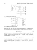
time between rising edges of P
E
) and T
I
(the time between rising edge of P
E
and trailing edge
of P
I
) are measured by the unit, as shown in Fig. 10. The phase difference is calculated from


2
180
C I
C
T T
T


  . (2)

This value is measured as average in averaging factor N
a
cycles of pulse signal P
E
. Thus, the
operating frequency is updated every N
a
cycles of the driving signals. The updated

operating frequency f
n+1
is given by







 rpnn
Kff
1
, (3)

where f
n
is the operating frequency before update,

r
is the admittance phase at resonance,


is the calculated admittance phase from eq. (2) (at a frequency of f
n
), K
p
is a proportional
feedback gain. To stabilize the tracing, K
p

should be selected as following inequality is
satisfied.


Fig. 7. Voltage/current detecting unit.


Fig. 8. Control unit with a microcomputer.

In
Hall
Element
Out
Amp/LPF Comp.
P
E
P
I
A
E
A
I
Micro Computer SH-7045F
PS/2
Keyboard
LCD
Display
COM
Port
EEPROM

24C16
P
E
A
E
A
I
P
I
MTU
AD Con
DDS

S
K
p
2
 , (4)

where S is the slope of the admittance phase vs. frequency curve at resonanse frequency.
The updated frequency is transmitted to the DDS. Repeating this routine, the operating
frequency can approach resonance frequency of transducer.

4. Application for Ultrasonic Dental Scaler

4.1 Ultrasonic dental scaler
Ultrasonic dental scaler is an equipment to remove dental calculi from teeth. the scaler
consists of a hand piece as shown in Fig. 10 and a driver circuit to excite vibration. A
Langevin type ultrasonic transducer is mounted in the hand piece. the structure of the
transducer is shown in Fig. 11. Piezoelectric elements are clamped by a tail block and a hone

block. A tip is attached on the top of the horn. The blocks and the tip are made of stainless
steel. The transducer vibrates longitudinally at first-order resonance frequency. One
vibration node is located in the middle. To support the node, the transducer is bound by a
silicon rubber.
To carry out the following experiments, a sample scaler was fabricated.Frequency response
of the electric charactorristics of the transducer was observed with no mechanical load and
input voltage of 20 V
p-p
. The result is shown in Fig. 12. From this result, the resonance
Fig. 9. Measurement of cycle and phase diference.
Fig. 10. Example of ultrasonic dental scalar hand piece.


Fig. 11. Structure of transducer for ultrasonic dental scalar.
P
E
P
I
T
C
T
I
Tip
Hand pieceHand piece
Tip
HornTail block
PZT
Rubber supporter
Tip
ResonanceFrequencyTracingSystemforLangevinTypeUltrasonicTransducers 111

time between rising edges of P
E
) and T
I
(the time between rising edge of P
E
and trailing edge
of P
I
) are measured by the unit, as shown in Fig. 10. The phase difference is calculated from


2
180
C I
C
T T
T


  . (2)

This value is measured as average in averaging factor N
a
cycles of pulse signal P
E
. Thus, the
operating frequency is updated every N
a
cycles of the driving signals. The updated

operating frequency f
n+1
is given by









 rpnn
Kff
1
, (3)

where f
n
is the operating frequency before update,

r
is the admittance phase at resonance,


is the calculated admittance phase from eq. (2) (at a frequency of f
n
), K
p
is a proportional

feedback gain. To stabilize the tracing, K
p
should be selected as following inequality is
satisfied.


Fig. 7. Voltage/current detecting unit.


Fig. 8. Control unit with a microcomputer.

In
Hall
Element
Out
Amp/LPF Comp.
P
E
P
I
A
E
A
I
Micro Computer SH-7045F
PS/2
Keyboard
LCD
Display
COM

Port
EEPROM
24C16
P
E
A
E
A
I
P
I
MTU
AD Con
DDS

S
K
p
2
 , (4)

where S is the slope of the admittance phase vs. frequency curve at resonanse frequency.
The updated frequency is transmitted to the DDS. Repeating this routine, the operating
frequency can approach resonance frequency of transducer.

4. Application for Ultrasonic Dental Scaler

4.1 Ultrasonic dental scaler
Ultrasonic dental scaler is an equipment to remove dental calculi from teeth. the scaler
consists of a hand piece as shown in Fig. 10 and a driver circuit to excite vibration. A

Langevin type ultrasonic transducer is mounted in the hand piece. the structure of the
transducer is shown in Fig. 11. Piezoelectric elements are clamped by a tail block and a hone
block. A tip is attached on the top of the horn. The blocks and the tip are made of stainless
steel. The transducer vibrates longitudinally at first-order resonance frequency. One
vibration node is located in the middle. To support the node, the transducer is bound by a
silicon rubber.
To carry out the following experiments, a sample scaler was fabricated.Frequency response
of the electric charactorristics of the transducer was observed with no mechanical load and
input voltage of 20 V
p-p
. The result is shown in Fig. 12. From this result, the resonance
Fig. 9. Measurement of cycle and phase diference.
Fig. 10. Example of ultrasonic dental scalar hand piece.


Fig. 11. Structure of transducer for ultrasonic dental scalar.
P
E
P
I
T
C
T
I
Tip
Hand pieceHand piece
Tip
HornTail block
PZT
Rubber supporter

Tip
MechatronicSystems,Simulation,ModellingandControl112
frequency was 31.93 kHz, admittance phase coincided with 0 at the resonance frequency,
electorical Q factor was 330 and the admittance phase response had a slope of -1 [deg/Hz]
in the neighborhood of the resonanse frequency.

4.2 Tracing test
Dental calculi are removed by contact with the tip. The applied voltage is adjusted
according to condition of the calculi. Temparature rises due to high applied voltage.
Therefore, during the operation, the resonance frequency of the transducer is shifted with
the changes of contact condition, temperature and amplitude of applied voltage. The
oscillating frequency was fixed in the conventional driving circuit. Consequently, vibration
amplitude was reduced due to the shift. The resonance frequency tracing system was apllied
to the ultrasonic dental scaler.

Fig. 12. Electric frequency response of the transducer for ultrasonic dental scalar.

Fig. 13. Step responses of the resonance frequency tracing system with the transducer for
ultrasonic dental scaler.
0
4
8
12
-90
0
90
31.7 31.8 31.9 32 32.1
Current [mA]
Admittance phase [deg]
Frequency [kHz]

Applied voltage: 20V
p-p
31.7
31.8
31.9
32
Time [ms]
Frequency [kHz]
K
P
= 1 / 2
K
P
= 1 / 4
K
P
= 1 / 16
K
P
= 1 / 8
Applied voltage: 20V
p-p
0 40 80 120 160
The transducer was driven by the tracing system, where averaging factor N
a
was set to 8. To
evaluate the system characteristic, step responses of the oscillating frequency were observed
in the same condition as the measurement of the electric frequency response. In this
measurement, initial operating frequency was 31.70 kHz. the frequency was differed from
the resonance frequency (31.93 kHz). At a time of 0 sec, the tracing was started. Namely, the

terget frecuency was changed, as a step input, to 31.93 kHz from 31.7 kHz. The transient
response of the oscillating frequency was observed. The oscillating frequency was measured
by a modulation domain analyzer in real time. Figure 13 shows the measurement results of
the responces. With each K
p
, the oscillating frequency in steady state was 31.93 kHz. the
frequency coincided with the resonance frequency. A settling time was 40 ms with K
p
of 1/4.
The settling time was evaluated from the time settled within ±2 % of steady state value. The
response speed is enough for the application to the dental scaler. Contact load does not
change faster than the response speed since the scaler is wielded by human. The
temperature and the amplitude of applied voltage also do not change so fast in normal
operation.

4.3 Dental diagnosis
When the transducer is contacted with an object, the natural frequency of the transdcer is
shifted. A value of the shift depends on stiffness and damping factor of the object
(Nishimura et. al, 1994). The contact model can be discribed as shown in Fig. 14. In this
model, the natural angular frequency of the transducer with contact is presented as


2
2
2
1















m
C
K
l
AE
m
C
C

, (5)

where m is the equivalent mass of the transducer, A is the section area of the transducer, E is
the elastic modulus of the material of the transducer, l is the half length of the transducer, K
c

is the stiffness of the object and C
c
is the damping coefficient of the object. Equation (5)
indicates that the combination factor of the damping factor and the stiffness can be
estimated from the natural frequency shift. The shift can be observed by the proposed

resonance frequency tracing system in real time. If the correlation between the combination
factor and the material properties is known, the damping factor or the stiffness of unknown
material can be predicted. For known materials, the local stiffness on the contacting point
can be estimated if the damping factor is assumed to be constant and known. Geometry also
can be evaluated from the estimated stiffness. For a dental health diagnosis, the stiffness

Fig. 14. Contact model of the transducer.
2l
Support point
Transducer Object
K
C
C
C
ResonanceFrequencyTracingSystemforLangevinTypeUltrasonicTransducers 113
frequency was 31.93 kHz, admittance phase coincided with 0 at the resonance frequency,
electorical Q factor was 330 and the admittance phase response had a slope of -1 [deg/Hz]
in the neighborhood of the resonanse frequency.

4.2 Tracing test
Dental calculi are removed by contact with the tip. The applied voltage is adjusted
according to condition of the calculi. Temparature rises due to high applied voltage.
Therefore, during the operation, the resonance frequency of the transducer is shifted with
the changes of contact condition, temperature and amplitude of applied voltage. The
oscillating frequency was fixed in the conventional driving circuit. Consequently, vibration
amplitude was reduced due to the shift. The resonance frequency tracing system was apllied
to the ultrasonic dental scaler.

Fig. 12. Electric frequency response of the transducer for ultrasonic dental scalar.

Fig. 13. Step responses of the resonance frequency tracing system with the transducer for
ultrasonic dental scaler.
0
4
8
12
-90
0
90
31.7 31.8 31.9 32 32.1
Current [mA]
Admittance phase [deg]
Frequency [kHz]
Applied voltage: 20V
p-p
31.7
31.8
31.9
32
Time [ms]
Frequency [kHz]
K
P
= 1 / 2
K
P
= 1 / 4
K
P
= 1 / 16

K
P
= 1 / 8
Applied voltage: 20V
p-p
0 40 80 120 160
The transducer was driven by the tracing system, where averaging factor N
a
was set to 8. To
evaluate the system characteristic, step responses of the oscillating frequency were observed
in the same condition as the measurement of the electric frequency response. In this
measurement, initial operating frequency was 31.70 kHz. the frequency was differed from
the resonance frequency (31.93 kHz). At a time of 0 sec, the tracing was started. Namely, the
terget frecuency was changed, as a step input, to 31.93 kHz from 31.7 kHz. The transient
response of the oscillating frequency was observed. The oscillating frequency was measured
by a modulation domain analyzer in real time. Figure 13 shows the measurement results of
the responces. With each K
p
, the oscillating frequency in steady state was 31.93 kHz. the
frequency coincided with the resonance frequency. A settling time was 40 ms with K
p
of 1/4.
The settling time was evaluated from the time settled within ±2 % of steady state value. The
response speed is enough for the application to the dental scaler. Contact load does not
change faster than the response speed since the scaler is wielded by human. The
temperature and the amplitude of applied voltage also do not change so fast in normal
operation.

4.3 Dental diagnosis
When the transducer is contacted with an object, the natural frequency of the transdcer is

shifted. A value of the shift depends on stiffness and damping factor of the object
(Nishimura et. al, 1994). The contact model can be discribed as shown in Fig. 14. In this
model, the natural angular frequency of the transducer with contact is presented as


2
2
2
1














m
C
K
l
AE
m
C

C

, (5)

where m is the equivalent mass of the transducer, A is the section area of the transducer, E is
the elastic modulus of the material of the transducer, l is the half length of the transducer, K
c

is the stiffness of the object and C
c
is the damping coefficient of the object. Equation (5)
indicates that the combination factor of the damping factor and the stiffness can be
estimated from the natural frequency shift. The shift can be observed by the proposed
resonance frequency tracing system in real time. If the correlation between the combination
factor and the material properties is known, the damping factor or the stiffness of unknown
material can be predicted. For known materials, the local stiffness on the contacting point
can be estimated if the damping factor is assumed to be constant and known. Geometry also
can be evaluated from the estimated stiffness. For a dental health diagnosis, the stiffness

Fig. 14. Contact model of the transducer.
2l
Support point
Transducer Object
K
C
C
C
MechatronicSystems,Simulation,ModellingandControl114
estimation can be applied. To discuss the possibility of the diagnosis, the frequency shifts
were measured using the experimental apparatus as shown in Fig. 15. A sample was

supported by an aluminum disk through a silicon rubber sheet. The transducer was fed by a
z-stage and contacted with the sample. The contact load was measured by load cells under
the aluminum disk. This measuring configuration was used in the following experiments.
The combination factor were observed in various materials. The natural frequency shifts in
contact with various materials were measured with the change of contact load. The shape
and size of the sample was rectangular solid and 20 mm x 20 mm x 5 mm except the LiNbO
3

sample. the size of the LiNbO
3
sample was 20 mm x 20 mm x 1 mm. The results are plotted
in Fig. 16. the natural frequency of the transducer decreased with the increase of contact
load in the case of soft material with high damping factor such as rubber. The natural
frequency did not change so much in the case of silicon rubber. The natural frequency
increased in the case of other materials. Comparing steel (SS400) and aluminum, stiffness of
steel is higher than that of aluminum. Frequency shift of LiNbO
3
is larger than that of steel
Fig. 15. Experimental apparatus for measurement of the frequency shifts with contact.


Fig. 16. Measurement of natural frequency shifts with the change of contact load in contact
with various materials.
Aluminum disk
Silicon rubber
sheet
Sample
Load cell
Contact load
Transducer

Supporting
part
-300
-200
-100
0
100
200
300
400
500
0 1 2 3 4 5 6
LiNbO
3
Steel (SS400)
Aluminium
Acrylic
Silicon rubber
Rubber

f [Hz]
Contact load [N]
Applied voltage: 20V
p-p
within 4 N though stiffness of LiNbO
3
is approximately same as that of steel. This means
that mechanical Q factor of LiNbO
3
is higher than that of steel, namely, damping factor of

LiNbO
3
is lower. Frequency shift of LiNbO
3
was saturated above 5 N. The reason can be
considered that effect of the silicon rubber sheet appeared in the measuring result due to
enough acoustic connection between the transducer and the LiNbO
3
.
The geometry was evaluated from local stiffness. The frequency shifts in contact with
aluminum blocks were measured with the change of contact load. The sample of the
aluminum block is shown in Fig. 17 (a). Three samples were used in the following
experiments. One of the samples had no hole, another had thickness t = 5 mm and the other
had the thickness t = 1 mm. Measured frequency shifts are shown in Fig. 17 (b). The
frequency shifts tended to be small with decrease of thickness t. These results show that the

Fig. 17. Measurement of natural frequency shifts with the change of contact load in contact
with aluminum blocks.

Fig. 18. Measurement of natural frequency shifts with the change of contact load in contact
with teeth.
(a)
f
20
f
10
t
20
0
50

100
150
200
250
300
350
0 1 2 3 4 5 6
No hole
5mm
1mm

f [Hz]
Contact load [N]
(b)
Applied voltage: 20V
p-p
Contact pointContact point
A
B
A
B
(a)
0
100
200
300
400
500
0 1 2 3 4 5 6


f [Hz]
Contact load [N]
Non-damaged (B)
(b)
Damaged (A)
Applied voltage: 20
V
p-p
ResonanceFrequencyTracingSystemforLangevinTypeUltrasonicTransducers 115
estimation can be applied. To discuss the possibility of the diagnosis, the frequency shifts
were measured using the experimental apparatus as shown in Fig. 15. A sample was
supported by an aluminum disk through a silicon rubber sheet. The transducer was fed by a
z-stage and contacted with the sample. The contact load was measured by load cells under
the aluminum disk. This measuring configuration was used in the following experiments.
The combination factor were observed in various materials. The natural frequency shifts in
contact with various materials were measured with the change of contact load. The shape
and size of the sample was rectangular solid and 20 mm x 20 mm x 5 mm except the LiNbO
3

sample. the size of the LiNbO
3
sample was 20 mm x 20 mm x 1 mm. The results are plotted
in Fig. 16. the natural frequency of the transducer decreased with the increase of contact
load in the case of soft material with high damping factor such as rubber. The natural
frequency did not change so much in the case of silicon rubber. The natural frequency
increased in the case of other materials. Comparing steel (SS400) and aluminum, stiffness of
steel is higher than that of aluminum. Frequency shift of LiNbO
3
is larger than that of steel
Fig. 15. Experimental apparatus for measurement of the frequency shifts with contact.

Fig. 16. Measurement of natural frequency shifts with the change of contact load in contact
with various materials.
Aluminum disk
Silicon rubber
sheet
Sample
Load cell
Contact load
Transducer
Supporting
part
-300
-200
-100
0
100
200
300
400
500
0 1 2 3 4 5 6
LiNbO
3
Steel (SS400)
Aluminium
Acrylic
Silicon rubber
Rubber


f [Hz]
Contact load [N]
Applied voltage: 20V
p-p
within 4 N though stiffness of LiNbO
3
is approximately same as that of steel. This means
that mechanical Q factor of LiNbO
3
is higher than that of steel, namely, damping factor of
LiNbO
3
is lower. Frequency shift of LiNbO
3
was saturated above 5 N. The reason can be
considered that effect of the silicon rubber sheet appeared in the measuring result due to
enough acoustic connection between the transducer and the LiNbO
3
.
The geometry was evaluated from local stiffness. The frequency shifts in contact with
aluminum blocks were measured with the change of contact load. The sample of the
aluminum block is shown in Fig. 17 (a). Three samples were used in the following
experiments. One of the samples had no hole, another had thickness t = 5 mm and the other
had the thickness t = 1 mm. Measured frequency shifts are shown in Fig. 17 (b). The
frequency shifts tended to be small with decrease of thickness t. These results show that the

Fig. 17. Measurement of natural frequency shifts with the change of contact load in contact
with aluminum blocks.

Fig. 18. Measurement of natural frequency shifts with the change of contact load in contact
with teeth.
(a)
f
20
f
10
t
20
0
50
100
150
200
250
300
350
0 1 2 3 4 5 6
No hole
5mm
1mm

f [Hz]
Contact load [N]
(b)
Applied voltage: 20V
p-p
Contact pointContact point
A
B

A
B
(a)
0
100
200
300
400
500
0 1 2 3 4 5 6

f [Hz]
Contact load [N]
Non-damaged (B)
(b)
Damaged (A)
Applied voltage: 20
V
p-p
MechatronicSystems,Simulation,ModellingandControl116
hollow in the contacted object can be investigated from the frequency shift even though
there is no difference in outward aspect.
Such elastic parameters estimation and the hollow investigation were applied for diagnosis
of dental health. The natural frequency shifts in contact with real teeth were also measured
on trial. Figure 18 (a) shows the teeth samples. Sample A is damaged by dental caries and B
is not damaged. The plotted points in the picture indicate contact points. To simulate real
environment, the teeth were supported by silicon rubber. Measured frequency shifts are
shown in Fig. 18 (b). It can be seen that the natural frequency shift of the damaged tooth is
smaller than that of healthy tooth.
Difference of resonance frequency shifts was observed. To conclude the possibility of dental

health diagnosis, a large number of experimental results were required. Collecting such
scientific date is our future work.

5. Conclusions

A resonance frequency tracing system for Langevin type ultrasonic transducers was built up.
The system configuration and the method of tracing were presented. The system does not
included a loop filter. This point provided easiness in the contoller design and availability
for various transducers.
The system was applied to an ultrasonic dental scaler. The traceability of the system with a
transducer for the scaler was evaluated from step responses of the oscillating frequency. The
settling time was 40 ms. Natural frequency shifts under tip contact with various object,
materials and geometries were observed. The shift measurement was applied to diagnosis of
dental health. Possibility of the diagnosis was shown.

6. References

Ide, M. (1968). Design and Analysis of Ultorasonic Wave Constant Velocity Control
Oscillator, Journal of the Institute of Electrical Engineers of Japan, Vol.88-11, No.962,
pp.2080-2088.
Si, F. & Ide, M. (1995). Measurement on Specium Acousitic Impedamce in Ultrsonic Plastic
Welding, Japanese Journal of applied physics, Vol.34, No.5B, pp.2740-2744.
Shimizu, H., Saito, S. (1978). Methods for Automatically Tracking the Transducer Resonance
by Rectified-Voltage Feedback to VCO, IEICE Technical Report, Vol.US78, No.173,
pp.7-13.
Hayashi, S. (1991). On the tracking of resonance and antiresonance of a piezoelectric
resonator, IEEE Transactions on. Ultrasonic, Ferroelectrics and Frequency Control,
Vol.38, No.3, pp.231-236.
Hayashi, S. (1992). On the tracking of resonance and antiresonance of a piezoelectric
resonator. II. Accurate models of the phase locked loop, IEEE Transactions on.

Ultrasonic, Ferroelectrics and Frequency Control, Vol.39, No.6, pp.787-790.
Aoyagi, R. & Yoshida, T. (2005), Unified Analysis of Frequency Equations of an Ultrasonic
Vibrator for the Elastic Sensor, Ultrasonic Technology, Vol.17, No.1, pp. 27-32.
Nishimura, K. et al., (1994), Directional Dependency of Sensitivity of Vibrating Touch sensor,
Proceedings of Japan Society of Precision Engineering Spring Conference, pp. 765-
766.
NewvisualServoingcontrolstrategiesintrackingtasksusingaPKM 117
NewvisualServoingcontrolstrategiesintrackingtasksusingaPKM
A.Traslosheros,L.Angel,J.M.Sebastián,F.Roberti,R.CarelliandR.Vaca
X

New visual Servoing control strategies in
tracking tasks using a PKM

i
A. Traslosheros,
ii
L. Angel,
i
J. M. Sebastián,

iii
F. Roberti,
iii
R. Carelli and
i
R. Vaca
i
DISAM, Universidad Politécnica de Madrid, Madrid, España,
ii

Facultad de Ingeniera
Electrónica Universidad Pontificia Bolivariana Bucaramanga, Colombia,
iii
Instituto de
Automática, Universidad Nacional de San Juan, San Juan, Argentina

1. Introduction

Vision allows a robotic system to obtain a lot of information on the surrounding
environment to be used for motion planning and control. When the control is based on
feedback of visual information is called Visual Servoing. Visual Servoing is a powerful tool
which allows a robot to increase its interaction capabilities and tasks complexity. In this
chapter we describe the architecture of the Robotenis system in order to design two different
control strategies to carry out tracking tasks. Robotenis is an experimental stage that is
formed of a parallel robot and vision equipment. The system was designed to test joint
control and Visual Servoing algorithms and the main objective is to carry out tasks in three
dimensions and dynamical environments. As a result the mechanical system is able to
interact with objects which move close to

2m=s
. The general architecture of control
strategies is composed by two intertwined control loops: The internal loop is faster and
considers the information from the joins, its sample time is
0:5ms
. Second loop represents
the visual Servoing system and it is an external loop to the first mentioned. The second loop
represents the main study purpose, it is based in the prediction of the object velocity that is
obtained from visual information and its sample time is
8:3ms
. The robot workspace

analysis plays an important role in Visual Servoing tasks, by this analysis is possible to
bound the movements that the robot is able to reach. In this article the robot jacobian is
obtained by two methods. First method uses velocity vector-loop equations and the second
is calculated from the time derivate of the kinematical model of the robot. First jacobian
requires calculating angles from the kinematic model. Second jacobian instead, depends on
physical parameters of the robot and can be calculated directly. Jacobians are calculated
from two different kinematic models, the first one determines the angles each element of the
robot. Fist jacobian is used in the graphic simulator of the system due to the information that
can be obtained from it. Second jacobian is used to determine off-line the work space of the
robot and it is used in the joint and visual controller of the robot (in real time). The work
space of the robot is calculated from the condition number of the jacobian (this is a topic that
is not studied in article). The dynamic model of the mechanical system is based on Lagrange
multipliers, and it uses forearms and end effector platform of non-negligible inertias for the
8
MechatronicSystems,Simulation,ModellingandControl118
development of control strategies. By means of obtaining the dynamic model, a nonlinear
feed forward and a PD control is been applied to control the actuated joints. High
requirements are required to the robot. Although requirements were taken into account in
the design of the system, additional protection is added by means of a trajectory planner. the
trajectory planner was specially designed to guarantee soft trajectories and protect the
system from exceeding its Maximum capabilities. Stability analysis, system delays and
saturation components has been taken into account and although we do not present real
results, we present two cases: Static and dynamic. In previous works (Sebastián, et al. 2007)
we present some results when the static case is considered.
The present chapter is organized as follows. After this introduction, a brief background is
exposed. In the third section of this chapter several aspects in the kinematic model, robot
jacobians, inverse dynamic and trajectory planner are described. The objective in this section
is to describe the elements that are considered in the joint controller. In the fourth section the
visual controller is described, a typical control law in visual Servoing is designed for the
system: Position Based Visual Servoing. Two cases are described: static and dynamic. When

the visual information is used to control a mechanical system, usually that information has
to be filtered and estimated (position and velocity). In this section we analyze two critical
aspects in the Visual Servoing area: the stability of the control law and the influence of the
estimated errors of the visual information in the error of the system. Throughout this
section, the error influence on the system behaviour is analyzed and bounded.

2. Background

Vision systems are becoming more and more frequently used in robotics applications. The
visual information makes possible to know about the position and orientation of the objects
that are presented in the scene and the description of the environment and this is achieved
with a relative good precision. Although the above advantages, the integration of visual
systems in dynamical works presents many topics which are not solved correctly yet. Thus
many important investigation centers (Oda, Ito and Shibata 2009) (Kragic and I. 2005) are
motivated to investigate about this field, such as in the Tokyo University ( (Morikawa, et al.
2007), (Kaneko, et al. 2005) and (Senoo, Namiki and Ishikawa 2004) ) where fast tracking (up
to
6m=s and 58m=s
2
) strategies in visual servoing are developed. In order to study and
implementing the different strategies of visual servoing, the computer vision group of the
UPM (Polytechnic University of Madrid) decided to design the Robotenis vision-robot
system. Robotenis system was designed in order to study and design visual servoing
controllers and to carry out visual robot tasks, specially, those involved in tracking where
dynamic environments are considered. The accomplishment of robotic tasks involving
dynamical environments requires lightweight yet stiff structures, actuators allowing for
high acceleration and high speed, fast sensor signal processing, and sophisticated control
schemes which take into account the highly nonlinear robot dynamics. Motivated by the
above reasons we proposed to design and built a high-speed parallel robot equipped with a
vision system.

a)
Fi
g

T
h
th
e
ev
a
s
ys
R
o
th
e
re
a
o
n
pr
e
S
y
ha
m
e
se
l
se

l

3.


B
a
ac
q
ef
f
th
i
co
n
th
e
g
. 1. Robotenis s
y
h
e Robotenis S
y
st
e
development o
f
a
luate the level
s

tem in applica
t
o
botenis S
y
stem i
s
e
vision s
y
stem
a
so
n
s that motiv
a
n
the performanc
e
e
cision of the m
o
stem have been
p
s been optimize
d
e
thod solved t
w
l

ectin
g
the actua
t
l
ected.

Robotenis de
s
a
sicall
y
, the Rob
o
q
uisition s
y
stem
.
f
ector speed is 4
m
i
s article reside
s
n
siderin
g
static
a

e
camera and t
h
y
stem and its env
i
em was created
t
f
a tool in order
of inte
g
ration b
e
t
ions with hi
g
h
s
inspired b
y
the

is based in one
a
te us the choic
e
e
of the s
y

stem,
o
vements. The ki
n
p
resented b
y
A
n
d
from the view o
w
o difficulties:
d
t
ors. In additio
n
s
cription
o
tenis platform

.
The parallel ro
b
m
=s. The visual
s
s
in tracking a

a
nd d
y
namic cas
e
h
e ball is const
a
i
ronment: Robot,

t
akin
g
into accou
n
to use in visual
s
e
tween a hi
g
h-s
p
temporar
y
requ
i

DELTA robot (
C

camera allocate
d
e
of the robot is
a
especiall
y
with
r
n
ematic anal
y
sis
a
ng
el, et al. (An
g
e
l
f both kinematic
s
d
eterminin
g
the
n
, the vision s
y
st
e

(Fig. 1.a) is for
m
b
ot is based on
a
sy
stem is based
o
black pin
g
pon
g
e
. Static case con
s
a
nt. D
y
namic ca
s

b)
c)

camera, back
g
r
o
n
t mainly two p

u
s
ervoin
g
researc
h
p
eed parallel ma
i
rements. The
m
C
lavel 1988) (Sta
m
d
at the end eff
e
a
consequence of

r
e
g
ard to velocit
y
a
nd the optimal
d
l
, et al. 2005). Th

e
s
and d
y
namics r
dime
n
sions of
t
e
m and the con
t
m
ed b
y
a paral
l
a
DELTA robot
a
o
n a camera in h
a
g
ball. Visual c
s
iders that the d
e
s
e considers th

a
o
und, ball and pa
d
u
rposes. The firs
t
h
. The second o
n
nipulator and a
m
echanical struc
t
m
per and Tsai 19
9
e
ctor of the rob
o

the hi
g
h requir
e
y
, acceleration a
n
d
esi

g
n of the Ro
b
e
structure of th
e
espectivel
y
. The
d
t
he parallel rob
o
t
rol hardware w
a
l
el robot a
n
d a
a
nd its maximu
m
a
nd and its ob
j
e
c
ontrol is desi
gn

e
sired distance b
e
a
t the desired d
i


d
dle.
t
one is
n
e is to
vision
t
ure of
9
7) and
o
t. The
e
ments
n
d the
b
otenis
e
robot
d

esi
g
n
o
t and
a
s also
visual
m
end-
c
tive in
n
ed by
e
tween
i
stance
NewvisualServoingcontrolstrategiesintrackingtasksusingaPKM 119
development of control strategies. By means of obtaining the dynamic model, a nonlinear
feed forward and a PD control is been applied to control the actuated joints. High
requirements are required to the robot. Although requirements were taken into account in
the design of the system, additional protection is added by means of a trajectory planner. the
trajectory planner was specially designed to guarantee soft trajectories and protect the
system from exceeding its Maximum capabilities. Stability analysis, system delays and
saturation components has been taken into account and although we do not present real
results, we present two cases: Static and dynamic. In previous works (Sebastián, et al. 2007)
we present some results when the static case is considered.
The present chapter is organized as follows. After this introduction, a brief background is
exposed. In the third section of this chapter several aspects in the kinematic model, robot

jacobians, inverse dynamic and trajectory planner are described. The objective in this section
is to describe the elements that are considered in the joint controller. In the fourth section the
visual controller is described, a typical control law in visual Servoing is designed for the
system: Position Based Visual Servoing. Two cases are described: static and dynamic. When
the visual information is used to control a mechanical system, usually that information has
to be filtered and estimated (position and velocity). In this section we analyze two critical
aspects in the Visual Servoing area: the stability of the control law and the influence of the
estimated errors of the visual information in the error of the system. Throughout this
section, the error influence on the system behaviour is analyzed and bounded.

2. Background

Vision systems are becoming more and more frequently used in robotics applications. The
visual information makes possible to know about the position and orientation of the objects
that are presented in the scene and the description of the environment and this is achieved
with a relative good precision. Although the above advantages, the integration of visual
systems in dynamical works presents many topics which are not solved correctly yet. Thus
many important investigation centers (Oda, Ito and Shibata 2009) (Kragic and I. 2005) are
motivated to investigate about this field, such as in the Tokyo University ( (Morikawa, et al.
2007), (Kaneko, et al. 2005) and (Senoo, Namiki and Ishikawa 2004) ) where fast tracking (up
to
6m=s and 58m=s
2
) strategies in visual servoing are developed. In order to study and
implementing the different strategies of visual servoing, the computer vision group of the
UPM (Polytechnic University of Madrid) decided to design the Robotenis vision-robot
system. Robotenis system was designed in order to study and design visual servoing
controllers and to carry out visual robot tasks, specially, those involved in tracking where
dynamic environments are considered. The accomplishment of robotic tasks involving
dynamical environments requires lightweight yet stiff structures, actuators allowing for

high acceleration and high speed, fast sensor signal processing, and sophisticated control
schemes which take into account the highly nonlinear robot dynamics. Motivated by the
above reasons we proposed to design and built a high-speed parallel robot equipped with a
vision system.
a)
Fi
g

T
h
th
e
ev
a
s
ys
R
o
th
e
re
a
o
n
pr
e
S
y
ha
m

e
se
l
se
l

3.


B
a
ac
q
ef
f
th
i
co
n
th
e
g
. 1. Robotenis s
y
h
e Robotenis S
y
st
e
development o

f
a
luate the level
s
tem in applicat
o
botenis S
y
stem i
s
e
vision s
y
stem
a
so
n
s that motiv
a
n
the performanc
e
e
cision of the m
o
stem have been
p
s been optimize
d
e

thod solved t
w
l
ectin
g
the actua
t
l
ected.

Robotenis de
s
a
sicall
y
, the Rob
o
q
uisition system.
f
ector speed is 4
m
i
s article reside
s
n
sidering static
a
e
camera and t

h
y
stem and its env
i
em was created
t
f
a tool in order
of inte
g
ration b
e
t
ions with high
s
inspired b
y
the

is based in one
a
te us the choic
e
e
of the s
y
stem,
o
vements. The ki
n

p
resented b
y
A
n
d
from the view o
w
o difficulties:
d
t
ors. In additio
n
s
cription
o
tenis platform

.
The parallel ro
b
m
=s. The visual
s
s
in tracking a
a
nd dynamic cas
e
h

e ball is const
a
i
ronment: Robot,

t
akin
g
into accou
n
to use in visual
s
e
tween a hi
g
h-s
p
temporary requ
i

DELTA robot (
C
camera allocate
d
e
of the robot is
a
especiall
y
with

r
n
ematic anal
y
sis
a
ng
el, et al. (An
g
e
l
f both kinematic
s
d
eterminin
g
the
n
, the vision s
y
st
e
(Fig. 1.a) is for
m
b
ot is based on
a
sy
stem is based
o

black pin
g
pon
g
e
. Static case con
s
a
nt. D
y
namic ca
s

b)
c)

camera, back
g
r
o
n
t mainly two p
u
s
ervoin
g
researc
h
p
eed parallel ma

i
rements. The
m
C
lavel 1988) (Sta
m
d
at the end eff
e
a
consequence of

r
e
g
ard to velocit
y
a
nd the optimal
d
l
, et al. 2005). Th
e
s
and d
y
namics r
dime
n
sions of

t
e
m and the con
t
m
ed b
y
a paral
l
a
DELTA robot
a
o
n a camera in h
a
g
ball. Visual c
s
iders that the d
e
s
e considers th
a
o
und, ball and pa
d
u
rposes. The firs
t
h

. The second o
n
nipulator and a
m
echanical struct
m
per and Tsai 19
9
e
ctor of the rob
o

the hi
g
h requir
e
y
, acceleration a
n
d
esi
g
n of the Ro
b
e
structure of th
e
espectivel
y
. The

d
t
he parallel rob
o
t
rol hardware w
a
l
el robot a
n
d a
a
nd its maximu
m
a
nd and its ob
j
e
c
ontrol is desi
gn
e
sired distance b
e
a
t the desired d
i


d

dle.
t
one is
n
e is to
vision
t
ure of
9
7) and
o
t. The
e
ments
n
d the
b
otenis
e
robot
d
esi
g
n
o
t and
a
s also
visual
m

end-
c
tive in
n
ed by
e
tween
i
stance
MechatronicSystems,Simulation,ModellingandControl120
between the ball and the camera can be changed at any time. Image processing is
conveniently simplified using a black ball on white background. The ball is moved through
a stick (Fig. 1.c) and the ball velocity is close to
2m=s
. The visual system of the Robotenis
platform is formed by a camera located at the end effector (Fig. 1.b) and a frame grabber
(SONY XC-HR50 and Matrox Meteor 2-MC/4 respectively) The motion system is formed by
AC brushless servomotors, Ac drivers (Unidrive) and gearbox.


Fig. 2. Cad model and sketch of the robot that it is seen from the side of the i-arm
In section 3.1

3.1 Robotenis kinematical models
A parallel robot consists of a fixed platform that it is connected to an end effector platform
by means of legs. These legs often are actuated by prismatic or rotating joints and they are
connected to the platforms through passive joints that often are spherical or universal. In the
Robotenis system the joints are actuated by rotating joints and connexions to end effector are
by means of passive spherical joints. If we applied the Grüble criterion to the Robotenis
robot, we could note that the robot has 9 DOF (this is due to the spherical joints and the

chains configurations) but in fact the robot has 3 translational DOF and 6 passive DOF.
Important differences with serial manipulators are that in parallel robots any two chains
form a closed loop and that the actuators often are in the fixed platform. Above means that
parallel robots have high structural stiffness since the end effector is supported in several
points at the same time. Other important characteristic of this kind of robots is that they are
able to reach high accelerations and forces, this is due to the position of the actuators in the
fixed platform and that the end effector is not so heavy in comparison to serial robots.
Although the above advantages, parallel robots have important drawbacks: the work space
is generally reduced because of collisions between mechanical components and that
singularities are not clear to identify. In singularities points the robot gains or losses degrees
of freedom and is not possible to control. We will see that the Jacobian relates the actuators
velocity with the end effector velocity and singularities occur when the Jacobian rank drops.
Nowadays there are excellent references to study in depth parallel robots, (Tsai 1999),
(Merlet 2006) and recently (Bonev and Gosselin 2009).
For the position analysis of the robot of the Robotenis system two models are presented in
order to obtain two different robot jacobians. As was introduced, the first jacobian is utilized
in the Robotenis graphic simulator and second jacobian is utilized in real time tasks.
Considers the Fig. 2, in this model we consider two reference systems. In the coordinate
system 

are represented the absolute coordinates of the system and the position  of
the end effector of the robot. In the local coordinate system 


(allocated in each point 

)
the position and coordinates (






) of the i-arm are considered. The first kinematic
model is calculated from Fig. 2 where the loop-closure equation for each limb is:

A
B B C O P PC O A
i i i i x y z i x y z i
   

    
(1)

Expressing (note that and the eq. (1) in the coordinate system
attached to each limb is possible to obtain:







 
     
   

   



 
 



 


 




 


 

 
 


1 3 1 2
3
1 3 1 2
a c b s c
C
i i i i
i x
C b c

i y i
C
a s b s s
i z
i i i i
(2)

Where  and 

are related by





   
 
 
 


   

 



 



   


 


   
 



 


   


 


   



   


 
c s 0
s c 0 0

0
0 0 1
P C h H
i i
x ix i i
P C
y i i iy
P C
z iz
(3)

In order to calculate the inverse kinematics, from the second row in eq. (2), we have:



 

 

 
 
1
c
3
C
i
y
i
b
i

(4)



can be obtained by summing the squares of 



and 

of the eq. (2).





 
    
  
2 2 2 2 2
2 c
3 2
C C C a b a b s
i x i y i z i i
→
 
2 2 2 2 2
1
c
2

2
3
C C C a b
ix iy iz
i
a b s
i


 
   
  
 


 
 
 

(5)

By expanding left member of the first and third row of the eq. (2) by using trigonometric
identities and making 














and



 











:
NewvisualServoingcontrolstrategiesintrackingtasksusingaPKM 121
between the ball and the camera can be changed at any time. Image processing is
conveniently simplified using a black ball on white background. The ball is moved through
a stick (Fig. 1.c) and the ball velocity is close to
2m=s
. The visual system of the Robotenis
platform is formed by a camera located at the end effector (Fig. 1.b) and a frame grabber

(SONY XC-HR50 and Matrox Meteor 2-MC/4 respectively) The motion system is formed by
AC brushless servomotors, Ac drivers (Unidrive) and gearbox.


Fig. 2. Cad model and sketch of the robot that it is seen from the side of the i-arm
In section 3.1

3.1 Robotenis kinematical models
A parallel robot consists of a fixed platform that it is connected to an end effector platform
by means of legs. These legs often are actuated by prismatic or rotating joints and they are
connected to the platforms through passive joints that often are spherical or universal. In the
Robotenis system the joints are actuated by rotating joints and connexions to end effector are
by means of passive spherical joints. If we applied the Grüble criterion to the Robotenis
robot, we could note that the robot has 9 DOF (this is due to the spherical joints and the
chains configurations) but in fact the robot has 3 translational DOF and 6 passive DOF.
Important differences with serial manipulators are that in parallel robots any two chains
form a closed loop and that the actuators often are in the fixed platform. Above means that
parallel robots have high structural stiffness since the end effector is supported in several
points at the same time. Other important characteristic of this kind of robots is that they are
able to reach high accelerations and forces, this is due to the position of the actuators in the
fixed platform and that the end effector is not so heavy in comparison to serial robots.
Although the above advantages, parallel robots have important drawbacks: the work space
is generally reduced because of collisions between mechanical components and that
singularities are not clear to identify. In singularities points the robot gains or losses degrees
of freedom and is not possible to control. We will see that the Jacobian relates the actuators
velocity with the end effector velocity and singularities occur when the Jacobian rank drops.
Nowadays there are excellent references to study in depth parallel robots, (Tsai 1999),
(Merlet 2006) and recently (Bonev and Gosselin 2009).
For the position analysis of the robot of the Robotenis system two models are presented in
order to obtain two different robot jacobians. As was introduced, the first jacobian is utilized

in the Robotenis graphic simulator and second jacobian is utilized in real time tasks.
Considers the Fig. 2, in this model we consider two reference systems. In the coordinate
system 

are represented the absolute coordinates of the system and the position  of
the end effector of the robot. In the local coordinate system 


(allocated in each point 

)
the position and coordinates (





) of the i-arm are considered. The first kinematic
model is calculated from Fig. 2 where the loop-closure equation for each limb is:

A
B B C O P PC O A
i i i i x y z i x y z i
   
     
(1)

Expressing (note that and the eq. (1) in the coordinate system
attached to each limb is possible to obtain:







 
     
   

   
 
 
 

 
 
 
 


 
 
 
 

 
 
 
1 3 1 2

3
1 3 1 2
a c b s c
C
i i i i
i x
C b c
i y i
C
a s b s s
i z
i i i i
(2)

Where  and 

are related by





   
 
 
 
 
   

 


 
 
 
   
 
 
 
   
 

 
 
 
   
 
 
 
   
 

   
 
 
c s 0
s c 0 0
0
0 0 1
P C h H
i i

x ix i i
P C
y i i iy
P C
z iz
(3)

In order to calculate the inverse kinematics, from the second row in eq. (2), we have:



 

 

 
 
1
c
3
C
i y
i
b
i
(4)



can be obtained by summing the squares of 




and 

of the eq. (2).





 
    
  
2 2 2 2 2
2 c
3 2
C C C a b a b s
i x i y i z i i
→
 
2 2 2 2 2
1
c
2
2
3
C C C a b
ix iy iz
i

a b s
i


 
   
  
 


 
 
 

(5)

By expanding left member of the first and third row of the eq. (2) by using trigonometric
identities and making 














and



 











:
MechatronicSystems,Simulation,ModellingandControl122
 
 
  

  

c( ) s( )
1 1
s( ) ( )
1 1
C

i i i i ix
c C
i i i i iz
(6)

Note that from (6) we can obtain:


 
 
 
 

 
 
 
( )
1
2 2
C C
i iz i ix
s
i
i i
and

 
 
 
 


 
 
 
( )
1
2 2
C C
i ix i iz
c
i
i i

(7)

Equations in (7) can be related to obtain ߠ
ଵ௜
as:


 
 
 

 

 
 
 
 

1
tan
1
C C
i iz i ix
i
C C
i ix i iz
(8)

In the use of above angles we have to consider that the “Z” axis that is attached to the center
of the fixed platform it is negative in the space that the end effector of the robot will be
operated. Taking into account the above consideration, angles are calculated as:

1
c
3
C
i
y
i
b


 

 

 
 

 
2 2 2 2 2
1
c
2
2
3
C C C a b
ix iy iz
i
a b s
i


 
   
  
 


 
 
 

1
tan
1
C C
i iz i ix

i
C C
i ix i iz

 
 
 

 

 
 
 
 
(9)

Second kinematic model is obtained from Fig. 3.

Fig. 3. Sketch of the robot taking into account an absolute coordinate reference system.

If we consider only one absolute coordinate system in Fig. 3, note that the segment ܤ
௜
ܥ
௜
is
the radius of a sphere that has its center in the point ܤ
௜
and its surface in the pointܥ
௜
, (all

points in the absolute coordinate system). Thus sphere equation as:
P
θ
1i
a
b
B
i
0
xyz
X
A
i
Y
ø
i

H
i
C
i
h
i
Z
 


 
2
2 2

2
0C B C B C B b
i ix ix iy iy iz iz

       
(10)

From the Fig. 3 is possible to obtain the point
B
i
=
O
x y z
B
i
in the absolute coordinate
system.

 
 
 
 
 
 
 
c c
c s
s
O
x y z

H a
B
i i i
i x
B H a
i y i i i
B
a
i z
i








 


 


 
 


 



 
 


where µ
i
= µ
1i

(11)

Replacing eq. (11) in eq. (10) and expanding it the constraint equationࢣ
࢏
is obtained:








  
     
2 2 2 2 2 2
2 c 2 s 2 c 2 c c
2 s 2 c s 0
H a b C C C H C H C H a a C
i i i x i

y
i z i i x i i i
y
i i i i x i i
a C a C
i z i i y i i

   
  
          
  
(12)

In order to simplify, above can be regrouped, thus for the i-limb:





s c 0E F M
i i i i i
 

 
(13)

Where:

   



   
 
2 c s 2
2 2 2 2 2 2
2 c s
F a C C H E a C
i i x i i y i i i i z
M b a C C C H H C C
i i x i y i z i i i x i i y i
 
 
   
       
(14)

The following trigonometric identities can be replaced into eq. (13):

 



 
 
 

 

 
 

1
2tan
2
s
1
2
1 tan
2
i
i
i
and
 



 

 
 

 

 
 
1
2
1 tan
2
c

1
2
1 tan
2
i
i
i
(15)

And we can obtain the following second order equation:

 
1 1
2
tan 2 tan 0
2 2
M F E M F
i i i i i i i
 
   

   
   
   
(16)

And the angle ߠ
௜
can be finally obtained as:
NewvisualServoingcontrolstrategiesintrackingtasksusingaPKM 123

 
 
  

  

c( ) s( )
1 1
s( ) ( )
1 1
C
i i i i ix
c C
i i i i iz
(6)

Note that from (6) we can obtain:


 
 


 

 
 
 
( )
1

2 2
C C
i iz i ix
s
i
i i
and

 
 


 

 
 
 
( )
1
2 2
C C
i ix i iz
c
i
i i

(7)

Equations in (7) can be related to obtain ߠ
ଵ௜

as:


 
 



 

 
 


 
1
tan
1
C C
i iz i ix
i
C C
i ix i iz
(8)

In the use of above angles we have to consider that the “Z” axis that is attached to the center
of the fixed platform it is negative in the space that the end effector of the robot will be
operated. Taking into account the above consideration, angles are calculated as:

1

c
3
C
i
y
i
b


 

 

 
 

 
2 2 2 2 2
1
c
2
2
3
C C C a b
ix iy iz
i
a b s
i



 
   
  
 


 
 
 

1
tan
1
C C
i iz i ix
i
C C
i ix i iz

 
 
 

 

 
 


 

(9)

Second kinematic model is obtained from Fig. 3.

Fig. 3. Sketch of the robot taking into account an absolute coordinate reference system.

If we consider only one absolute coordinate system in Fig. 3, note that the segment ܤ
௜
ܥ
௜
is
the radius of a sphere that has its center in the point ܤ
௜
and its surface in the pointܥ
௜
, (all
points in the absolute coordinate system). Thus sphere equation as:
P
θ
1i
a
b
B
i
0
xyz
X
A
i
Y

ø
i

H
i
C
i
h
i
Z
 
 
 
2
2 2
2
0C B C B C B b
i ix ix iy iy iz iz
        
(10)

From the Fig. 3 is possible to obtain the point
B
i
=
O
x y z
B
i
in the absolute coordinate

system.

 
 
 
 
 
 
 
c c
c s
s
O
x y z
H a
B
i i i
i x
B H a
i y i i i
B
a
i z
i
 
 

 

 

 
 
 
 
 
 
 
 
 
 
 
where µ
i
= µ
1i

(11)

Replacing eq. (11) in eq. (10) and expanding it the constraint equationࢣ
࢏
is obtained:








  

     
2 2 2 2 2 2
2 c 2 s 2 c 2 c c
2 s 2 c s 0
H a b C C C H C H C H a a C
i i i x i
y
i z i i x i i i
y
i i i i x i i
a C a C
i z i i y i i

   
  
          
  
(12)

In order to simplify, above can be regrouped, thus for the i-limb:





s c 0E F M
i i i i i
 
  
(13)

Where:

   


   
 
2 c s 2
2 2 2 2 2 2
2 c s
F a C C H E a C
i i x i i y i i i i z
M b a C C C H H C C
i i x i y i z i i i x i i y i
 
 
   
       
(14)

The following trigonometric identities can be replaced into eq. (13):

 



 
 
 


 

 
 
1
2tan
2
s
1
2
1 tan
2
i
i
i
and
 



 

 
 

 

 
 

1
2
1 tan
2
c
1
2
1 tan
2
i
i
i
(15)

And we can obtain the following second order equation:

 
1 1
2
tan 2 tan 0
2 2
M F E M F
i i i i i i i
 
   
    
   
   
(16)

And the angle ߠ
௜
can be finally obtained as:
MechatronicSystems,Simulation,ModellingandControl124


 
2 2 2
1
2 t a n
E E F M
i i i i
i
M F
i i

 
 
   
 
 


 
 

 
 
 
 

(17)

Where 



and 

are:


  
   
c s 0
s c 0 0
0
0 0 1
C P h
i i
i x x i
C P
i y y i i
C P
i z z
 
 
 
   



 
 
   
 
 
   
 
 
 
   
 
 
   
 
   
 
(18)

3.2 Robot Jacobians
In robotics, the robot Jacobian can be seen as the linear relation between the actuators
velocity and the end effector velocity. In Fig. 4. direct and inverse Jacobian show them
relation with the robot speeds. Although the jacobian can be obtained by other powerful
methods (screws theory (Stramigioli and Bruyninckx 2001) (Davidson and Hunt Davidson
2004) or motor algebra (Corrochano and Kähler 2000)), conceptually the robot jacobian can
be obtained as the derivate of the direct or the inverse kinematic model. In parallel robots
the obtaining of the Jacobian by means of the screws theory or motor algebra can be more
complicated. This complication is due to its non actuated joints (that they are not necessary
passive joints). The easier method to understand, but not to carry out, is to derivate respect
the time the kinematic model of the robot.

Fig. 4. Direct and indirect Jacobian and its relation with the robot velocities

Sometimes is more complex to obtain the inverse or direct Jacobian from one kinematic
model than other thus, in some practical cases is possible to obtain the inverse Jacobian by
inverting the direct Jacobian and vice versa, Fig. 4. Above proposal is easy to describe but
does not analyze complications. For example if we would like to calculate the inverse
Jacobian form the direct Jacobian, we have to find the inverse of a matrix that its dimension
is normally . This matrix inversion it could be very difficult because components of the
Jacobian are commonly complex functions and composed by trigonometric functions.
Alternatively it is possible to calculate the inverse Jacobian or the direct Jacobian by other
methods. For example if we have the algebraic form of the direct Jacobian, we could
calculate the inverse of the Jacobian by means of inverting the numeric direct Jacobian
(previously evaluated at one point). On the other hand the Jacobian gives us important
Velocities of the end
effector of the robot












Velocities of the
actuated joints













(Inverse Jacobian)
-1
Direct Jacobian
Inverse Jacobian
(Direct Jacobian)
-1
information about the robot, from the Jacobian we can determinate when a singularity
occurs. There are different classifications for singularities of a robot. Some singularities can
be classified according to the place in the space where they occurs (singularities can present
on the limit or inside of the workspace of the robot). Another classification takes into
account how singularities are produced (produced from the direct or inverse kinematics).
Suppose that the eq. (19) describes the kinematics restrictions that are imposed to
mechanical elements (joints, arms, lengths, etc.) of the robot.



, 0f x q


(19)

Where 

is the position and orientation of the end effector of the robot and


are the joint variables that are actuated. Note that if  the robot is redundant and
if  the robot cannot fully orientate () or displace (along) in the 3D space.
Although sometimes a robot can be specially designed with other characteristics, in general
a robot has the same number of DOF that its number of actuators.
Consider the time derivative of the eq. (19) in the following equation.

J x J q
x q

 
where


x, q
x
x
f
J



and



x, q
q
q
f
J




(20)
Note that  and  are the time derivate of  and  respectely. The direct and the inverse
Jacobian can be obtained as the following equations.

x J
q
D

 
and
q
J x
I

 
where




1
J
J J
D x
q
and


1
J
J J
I
q
x

(21)

A robot singularity occurs when the determinant of the Jacobian is cero. Singularities can be
divided in three groups: singularities that are due to the inverse kinematics, those that are
due to the direct kinematics and those that occurs when both above singularities take place
at the same time (combined singularities). For a non redundant robot (the Jacobian is a
square matrix), each one of above singularities happens when:

, 

 and
when 







. Singularities can be interpreted differently in serial robots and
in parallel robots. When we have that

, it means that the null space of 

is not
empty. That is, there are values of that are different from cero and produce an end effector
velocity that is equal to cero. In this case, the robot loses DOF because there are
infinitesimal movements of the joints that do not produce movement of the end effector;
commonly this occurs when robot links of a limb are in the same plane. Note that when an
arm is completely extended, the end effector can supported high loads when the action of
the load is in the same direction of the extended arm. On the other hand when 


we have a direct kinematics singularity, this means that the null space of 

is not empty.
The above means that there are values of that are different from cero when the actuators
are blocked . Physically, the end effector of the robot gains DOF. When the end effector
gains DOF is possible to move infinitesimally although the actuators would be blocked. The
third type of singularity it is a combined singularity and can occurs in parallel robots with
special architecture or under especial considerations. Sometimes singularities can be
NewvisualServoingcontrolstrategiesintrackingtasksusingaPKM 125


 
2 2 2

1
2 t a n
E E F M
i i i i
i
M F
i i



 
   
 




 



 


 


(17)

Where 




and 

are:


  
   
c s 0
s c 0 0
0
0 0 1
C P h
i i
i x x i
C P
i y y i i
C P
i z z
 
 
 
   




 

   


 
   
 


 
   


 
   


   
 
(18)

3.2 Robot Jacobians
In robotics, the robot Jacobian can be seen as the linear relation between the actuators
velocity and the end effector velocity. In Fig. 4. direct and inverse Jacobian show them
relation with the robot speeds. Although the jacobian can be obtained by other powerful
methods (screws theory (Stramigioli and Bruyninckx 2001) (Davidson and Hunt Davidson
2004) or motor algebra (Corrochano and Kähler 2000)), conceptually the robot jacobian can
be obtained as the derivate of the direct or the inverse kinematic model. In parallel robots
the obtaining of the Jacobian by means of the screws theory or motor algebra can be more
complicated. This complication is due to its non actuated joints (that they are not necessary
passive joints). The easier method to understand, but not to carry out, is to derivate respect

the time the kinematic model of the robot.


Fig. 4. Direct and indirect Jacobian and its relation with the robot velocities

Sometimes is more complex to obtain the inverse or direct Jacobian from one kinematic
model than other thus, in some practical cases is possible to obtain the inverse Jacobian by
inverting the direct Jacobian and vice versa, Fig. 4. Above proposal is easy to describe but
does not analyze complications. For example if we would like to calculate the inverse
Jacobian form the direct Jacobian, we have to find the inverse of a matrix that its dimension
is normally . This matrix inversion it could be very difficult because components of the
Jacobian are commonly complex functions and composed by trigonometric functions.
Alternatively it is possible to calculate the inverse Jacobian or the direct Jacobian by other
methods. For example if we have the algebraic form of the direct Jacobian, we could
calculate the inverse of the Jacobian by means of inverting the numeric direct Jacobian
(previously evaluated at one point). On the other hand the Jacobian gives us important
Velocities of the end
effector of the robot













Velocities of the
actuated joints












(Inverse Jacobian)
-1
Direct Jacobian
Inverse Jacobian
(Direct Jacobian)
-1
information about the robot, from the Jacobian we can determinate when a singularity
occurs. There are different classifications for singularities of a robot. Some singularities can
be classified according to the place in the space where they occurs (singularities can present
on the limit or inside of the workspace of the robot). Another classification takes into
account how singularities are produced (produced from the direct or inverse kinematics).
Suppose that the eq. (19) describes the kinematics restrictions that are imposed to
mechanical elements (joints, arms, lengths, etc.) of the robot.




, 0f x q 

(19)

Where 

is the position and orientation of the end effector of the robot and


are the joint variables that are actuated. Note that if  the robot is redundant and
if  the robot cannot fully orientate () or displace (along) in the 3D space.
Although sometimes a robot can be specially designed with other characteristics, in general
a robot has the same number of DOF that its number of actuators.
Consider the time derivative of the eq. (19) in the following equation.

J x J q
x q

 
where


x, q
x
x
f
J




and


x, q
q
q
f
J




(20)
Note that  and  are the time derivate of  and  respectely. The direct and the inverse
Jacobian can be obtained as the following equations.

x J q
D

 
and q J x
I

 
where



1
J

J J
D x
q
and


1
J
J J
I
q
x

(21)

A robot singularity occurs when the determinant of the Jacobian is cero. Singularities can be
divided in three groups: singularities that are due to the inverse kinematics, those that are
due to the direct kinematics and those that occurs when both above singularities take place
at the same time (combined singularities). For a non redundant robot (the Jacobian is a
square matrix), each one of above singularities happens when:

, 

 and
when 







. Singularities can be interpreted differently in serial robots and
in parallel robots. When we have that

, it means that the null space of 

is not
empty. That is, there are values of that are different from cero and produce an end effector
velocity that is equal to cero. In this case, the robot loses DOF because there are
infinitesimal movements of the joints that do not produce movement of the end effector;
commonly this occurs when robot links of a limb are in the same plane. Note that when an
arm is completely extended, the end effector can supported high loads when the action of
the load is in the same direction of the extended arm. On the other hand when 


we have a direct kinematics singularity, this means that the null space of 

is not empty.
The above means that there are values of that are different from cero when the actuators
are blocked . Physically, the end effector of the robot gains DOF. When the end effector
gains DOF is possible to move infinitesimally although the actuators would be blocked. The
third type of singularity it is a combined singularity and can occurs in parallel robots with
special architecture or under especial considerations. Sometimes singularities can be
MechatronicSystems,Simulation,ModellingandControl126
identified from the Jacobian almost directly but sometimes Jacobian elements are really
complex and singularities are difficult to identify. Singularities can be identified in easier
manner depending on how the Jacobian is obtained. The Robotenis Jacobian is obtained by
two methods, one it is obtained from the time derivate of a closure loop equation (1) and the
second Jacobian is obtained from the time derivate of the second kinematic model.
Remember that the jacobian obtained from the eq. (1) requires solving the kinematic model

in eqs. (9). This jacobian requires more information of each element of the robot and it is
used in the graphic simulator of the system. In order to obtain the jacobian consider that


and that the eq. (1) is rearranged as:

( , ) ( , )O P R z P C R z O A A B B C
i i i i i i i
 
 
   
     
 
(22)

Where 



is a rotation matrix around the  axis in the absolute coordinate system.

( ) ( ) 0
( , ) ( ) ( ) 0
0 0 1
c s
R z s c
 
  




 

 
 
 
(23)

By obtaining the time derivate of the equation (22) and multiplying by 




 we have:

( , )
1 2
T
R z P
i i i
  
   a b
i i

(24)
Where

is velocity of the end effector in the coordinate system, 

















, 



















and 

, 

are the angular velocities of the links  and  of the  limb. Observe that 

and


are passive variables (they are not actuated) thus to eliminate the passive joint speeds
(

) we dot multiply both sides of eq. (24) by

. By means of the properties of the triple
product (


 


 


  



 and


 


 





 


 


 ) is possible to obtain:

( , ) ( )
1
T
b R z P
i i
 
 
   
 
 

i i
a b

(25)

From Fig. 2 elements of above equation are:



 
1
0
1
c
i
a
s
i


 
 
 



 
 
a
i

;




 
   
3 1 2
3
3 1 2
s c
i i i
b c
i
s s
i i i
  

  
 

 
 

 
 

 
 
b

i
and
0
1 1
0
i i
 
 
 
 
 
 




(26)

All of them are expressed in the coordinate system. Substituting equations in (26) into
(25) and after operating and simplifying we have:
( ) ( ) 0 0
1 1 1
1 1
2 1 3 1
0 ( ) ( ) 0
2 2 2 22 3 2 1 2
0 0 ( ) ( )
2 3 3 3
1 3
3 3 3

m m m
P
s s
x y z
x
m m m P a s s
x y z y
s s
m m m
P
x y z
z

 
  
 

 
 


 
 
 


 
 
 




 
 
 


 
 
 


 
 


 
 
 
 


 



(27)

Where











         
   
1 2 3 3
1 2 3 3
1 2 3
m c s c c s
i x i i i i i i
m c s s c c
i y i i i i i i
m s s
i z i i i

    

    
  
  
  
 

(28)

Note that the right and left part of the eq. (27) represents the inverse and direct Jacobians
respectively. An inverse kinematic singularity occurs whenߠ
ଶ௜
ൌͲ݋ݎߨ or ߠ
ଷ௜
ൌͲ݋ݎߨ, see
Fig. 5 a) and b). On the other hand direct kinematic singularities occur when rows of the left
matrix become linearly dependent. The above is:

0
1 1 2 2 3 3
k m k m k m


   
  
   


Where
1
k
,
2
k
,
3
k



and not all are cero
(29)

Equation (29) is not as clear as the right part of the equation (27) but we can identify a
group of direct kinematic singularities when the last column in the three rows is cero, this is:

( ) ( ) ( ) ( ) ( ) ( ) 0
1 1 21 3 1 1 2 22 3 2 1 3 2 3 3 3
s s s s s s

       

    


When

0
1 2i i


 
or





1,2,3i
or when


0
3i
or




1,2,3i

(30)
a) b)
NewvisualServoingcontrolstrategiesintrackingtasksusingaPKM 127
identified from the Jacobian almost directly but sometimes Jacobian elements are really
complex and singularities are difficult to identify. Singularities can be identified in easier
manner depending on how the Jacobian is obtained. The Robotenis Jacobian is obtained by
two methods, one it is obtained from the time derivate of a closure loop equation (1) and the
second Jacobian is obtained from the time derivate of the second kinematic model.
Remember that the jacobian obtained from the eq. (1) requires solving the kinematic model
in eqs. (9). This jacobian requires more information of each element of the robot and it is
used in the graphic simulator of the system. In order to obtain the jacobian consider that


and that the eq. (1) is rearranged as:

( , ) ( , )O P R z P C R z O A A B B C
i i i i i i i

 


   

    


(22)

Where 



is a rotation matrix around the  axis in the absolute coordinate system.

( ) ( ) 0
( , ) ( ) ( ) 0
0 0 1
c s
R z s c
 
  













(23)

By obtaining the time derivate of the equation (22) and multiplying by 




 we have:

( , )
1 2
T
R z P
i i i
  
   a b
i i

(24)
Where

is velocity of the end effector in the coordinate system, 

















, 



















and 

, 

are the angular velocities of the links  and  of the  limb. Observe that 

and


are passive variables (they are not actuated) thus to eliminate the passive joint speeds
(

) we dot multiply both sides of eq. (24) by

. By means of the properties of the triple
product (


 


 


  


 and



 


 





 


 


 ) is possible to obtain:

( , ) ( )
1
T
b R z P
i i
 
 
   
 
 
i i

a b

(25)

From Fig. 2 elements of above equation are:



 
1
0
1
c
i
a
s
i
















a
i
;




 
   
3 1 2
3
3 1 2
s c
i i i
b c
i
s s
i i i
  

  


















b
i
and
0
1 1
0
i i
 




 








(26)

All of them are expressed in the coordinate system. Substituting equations in (26) into
(25) and after operating and simplifying we have:
( ) ( ) 0 0
1 1 1
1 1
2 1 3 1
0 ( ) ( ) 0
2 2 2 22 3 2 1 2
0 0 ( ) ( )
2 3 3 3
1 3
3 3 3
m m m
P
s s
x y z
x
m m m P a s s
x y z y
s s
m m m
P
x y z
z

 
  

 

 
 
 
 
 
 
 
 
 
 
 

 
 
 
 
 
 
 
 
 
 
 
 
 
 
 



 



(27)

Where











         
   
1 2 3 3
1 2 3 3
1 2 3
m c s c c s
i x i i i i i i
m c s s c c
i y i i i i i i
m s s
i z i i i

     
     
  
  
  
 

(28)

Note that the right and left part of the eq. (27) represents the inverse and direct Jacobians
respectively. An inverse kinematic singularity occurs whenߠ
ଶ௜
ൌͲ݋ݎߨ or ߠ
ଷ௜
ൌͲ݋ݎߨ, see
Fig. 5 a) and b). On the other hand direct kinematic singularities occur when rows of the left
matrix become linearly dependent. The above is:

0
1 1 2 2 3 3
k m k m k m
 
   
  
   
 
Where
1
k
,

2
k
,
3
k


and not all are cero
(29)

Equation (29) is not as clear as the right part of the equation (27) but we can identify a
group of direct kinematic singularities when the last column in the three rows is cero, this is:

( ) ( ) ( ) ( ) ( ) ( ) 0
1 1 21 3 1 1 2 22 3 2 1 3 2 3 3 3
s s s s s s

       
     


When

0
1 2i i
 
 
or



 1,2,3i
or when

0
3i
or



 1,2,3i

(30)
a) b)