Mechatronic Systems, Simulation, Modeling and Control Part 4 pptx
Bạn đang xem bản rút gọn của tài liệu. Xem và tải ngay bản đầy đủ của tài liệu tại đây (819.76 KB, 18 trang )
MechatronicSystems,Simulation,ModellingandControl128
c) d)
Fig. 5. a) Inverse kinematic singularities ifࣂ
ൌ࣊. b) Inverse kinematic singularities
whereࣂ
ൌǢൌǡǡ. c) Direct kinematic singularity ifࣂ
ࣂ
ൌ࣊Ǣൌǡǡ. d)
Combined kinematic singularity if ࣂ
ൌ࣊Ǣࣂ
ൌǢࣂ
ൌǢࣂ
ࣂ
ൌ࣊Ǣࣂ
ࣂ
ൌ
andࣘ
ࣘ
ൌ࢘࣊. Note that the robot presents a combined singularity if three
anglesࣂ
ൌ࣊Ǣൌǡǡ consequently case c) is a combined singularity (ࣂ
ൌǢࣂ
ൌ
). Note that the design of the robot plays a very important role because singularities can
even avoid. For example in figure c) the singularity is present because lengths of the forearm
allows to be in the same plane that the end effector platform and in the figure d) a combined
singularity is present becauseࣘ
ࣘ
ൌ. In all figures we suppose that the limb ൌ is
the limb situated to the left of the images. Note that collisions between mechanical elements
are not taken into account.
By considering (27) to (30), direct kinematic singularities present when the end effector
platform is in the same plane as the parallelograms of the 3 limbs, in this configuration the
robot cannot resist any load in the Z direction, see Fig. 5 c). Note that singularities like above
depend on the lengths and angles of the robot when it was designed Fig. 5 c), such is the
case of the above configuration where singularity can present whenࢇࡴ࢈ , other
singularities can present in special values ofࣘ
Fig. 5 d).
Analysis of singularities of the work space is important for Visual controller in order to
bound the workspace an avoid robot injures. Above analysis is useful because some
singularities are given analytically. Different views of the work space of the CAD model of
the Robotenis system is shown in Fig. 6
a) b) c)
Fig. 6 Work space of the Robotenis system. a) Work space is seen from bottom part of the
robot, b) it shows the workspace from side. c) The isometric view of the robot is shown.
As was mentioned a second jacobian is obtained to use in real time tasks, by the condition
number of the jacobian (Yoshikawa 1985) is possible to know how far a singularity is.
Condition number of the jacobian y checked before carry out any movement of the robot, if
a large condition number is present, then the movement is not carried out.
In order to obtain the second jacobian consider that we have the inverse kinematic model of
a robot in given by eq. (31).
, , , , ,
1 1
, , , , ,
q f x y z
q f x y z
n n
(31)
1
x
y
q
z
J
I
q
n
Where:
1
f f
n
x
J
I
f f
n n
x
(32)
Note that the kinematic model of the Robotenis system is formed by three equations in eq.
(17) (the end effector cannot orientate) and this model has the form of the eq. (31).
Consequently to obtain the jacobian we have to find the time derivate of the kinematic
model. Thus to simplify operations we suppose that.
2 2 2
E E F M
i i i i
t
i
M F
i i
(33)
And that in terms of ߰the time derivate of (17) is:
2
2
1
i
i
i
(34)
Where ߰
ሶ
is
2 2 2
2 2
2 2 2
E M F M F
P M F
E E E M M F F
i
M F
M F M F
M F E M F
i
(35)
Considering that ߟ
ଵ
ൌ
ଵ
ெିி
and ߟ
ଶ
ൌ
ଵ
ඥ
ா
మ
ି
ሺ
ெ
మ
ିி
మ
ሻ
can be replaced in (35).
2 2
2 2
1 1
1 1 1 1 2 1 2 1 2
2 2
M F
E E M E F E E M M F F
i
i
(36)
NewvisualServoingcontrolstrategiesintrackingtasksusingaPKM 129
c) d)
Fig. 5. a) Inverse kinematic singularities ifࣂ
ൌ࣊. b) Inverse kinematic singularities
whereࣂ
ൌǢൌǡǡ. c) Direct kinematic singularity ifࣂ
ࣂ
ൌ࣊Ǣൌǡǡ. d)
Combined kinematic singularity if ࣂ
ൌ࣊Ǣࣂ
ൌǢࣂ
ൌǢࣂ
ࣂ
ൌ࣊Ǣࣂ
ࣂ
ൌ
andࣘ
ࣘ
ൌ࢘࣊. Note that the robot presents a combined singularity if three
anglesࣂ
ൌ࣊Ǣൌǡǡ consequently case c) is a combined singularity (ࣂ
ൌǢࣂ
ൌ
). Note that the design of the robot plays a very important role because singularities can
even avoid. For example in figure c) the singularity is present because lengths of the forearm
allows to be in the same plane that the end effector platform and in the figure d) a combined
singularity is present becauseࣘ
ࣘ
ൌ. In all figures we suppose that the limb ൌ is
the limb situated to the left of the images. Note that collisions between mechanical elements
are not taken into account.
By considering (27) to (30), direct kinematic singularities present when the end effector
platform is in the same plane as the parallelograms of the 3 limbs, in this configuration the
robot cannot resist any load in the Z direction, see Fig. 5 c). Note that singularities like above
depend on the lengths and angles of the robot when it was designed Fig. 5 c), such is the
case of the above configuration where singularity can present whenࢇࡴ࢈ , other
singularities can present in special values ofࣘ
Fig. 5 d).
Analysis of singularities of the work space is important for Visual controller in order to
bound the workspace an avoid robot injures. Above analysis is useful because some
singularities are given analytically. Different views of the work space of the CAD model of
the Robotenis system is shown in Fig. 6
a) b) c)
Fig. 6 Work space of the Robotenis system. a) Work space is seen from bottom part of the
robot, b) it shows the workspace from side. c) The isometric view of the robot is shown.
As was mentioned a second jacobian is obtained to use in real time tasks, by the condition
number of the jacobian (Yoshikawa 1985) is possible to know how far a singularity is.
Condition number of the jacobian y checked before carry out any movement of the robot, if
a large condition number is present, then the movement is not carried out.
In order to obtain the second jacobian consider that we have the inverse kinematic model of
a robot in given by eq. (31).
, , , , ,
1 1
, , , , ,
q f x y z
q f x y z
n n
(31)
1
x
y
q
z
J
I
q
n
Where:
1
f f
n
x
J
I
f f
n n
x
(32)
Note that the kinematic model of the Robotenis system is formed by three equations in eq.
(17) (the end effector cannot orientate) and this model has the form of the eq. (31).
Consequently to obtain the jacobian we have to find the time derivate of the kinematic
model. Thus to simplify operations we suppose that.
2 2 2
E E F M
i i i i
t
i
M F
i i
(33)
And that in terms of ߰the time derivate of (17) is:
2
2
1
i
i
i
(34)
Where ߰
ሶ
is
2 2 2
2 2
2 2 2
E M F M F
P M F
E E E M M F F
i
M F
M F M F
M F E M F
i
(35)
Considering that ߟ
ଵ
ൌ
ଵ
ெିி
and ߟ
ଶ
ൌ
ଵ
ඥ
ா
మ
ି
ሺ
ெ
మ
ିி
మ
ሻ
can be replaced in (35).
2 2
2 2
1 1
1 1 1 1 2 1 2 1 2
2 2
M F
E E M E F E E M M F F
i
i
(36)
MechatronicSystems,Simulation,ModellingandControl130
On the other hand we know that:
2 c 2 s
2 2 2 2 c 2 s
2
F aC aC
i i x i i y i
M C C C C C C HC HC
i i x i x i y i y i z i z i x i i y i
E aC
i i z
(37)
By rearranging terms in eq. (36) and considering terms in (37) is possible to obtain ߰ in
terms of the velocity of the end effectorܥ
ሶ
௫௬௭
.
2 d C d C d C
i i x i x i
y
i
y
i z i z
(38)
Where:
2
c c
1
c c
1 2
2
1
c c
2
P C H a
x
M C F a M H
x
d
i x
a C H
x
i
,
2
1
1 2
2
1
2
P C H s as
y
F as M C M H s
y
d
i y
as C H s
y
i
,
1
1
1
2
2
a E C
z
d
i z
Pa M C C
z z
i
(39)
Then replacing eq. (38) in (34) we have:
4
2
2 2 2
1
2
d C d C d C
i x i x i y i y i z i z
i
E E F M
M F
i
and
4
C
i x
D D D C
i i x i
y
i z i
y
C
i z
(40)
Note that the actuator speed is in terms of the velocity of the point ܥ
and the time derivate
of ܥ
is:
c o s s i n 0
0
s i n c o s 0
0
0 0 1
1
h
C
P
i
i i
i x
x
d
C P
i y y i i
d t
P
C
z
i z
where ߶ is constant and
C P
ix x
C P
iy y
C P
iz z
(41)
Substituting the above equation in (40) and the expanding the equation, finally the inverse
Jacobian of the robot is given by:
1 1 1
1
4
2 2 2 2
3
3 3 3
D D D
P
x y z
x
D D D P
x y z y
D D D
P
x y z
z
(42)
Note that the robot Jacobian in eq. (42) has the advantage that is fully expressed in terms of
physical parameters of the robot and is not necessary to solve previously any kinematic
model. Terms in eq. (42) are complex and this make not easy to detect singularities by only
inspecting the expression. In the real time controller, the condition number of the jacobian is
calculated numerically to detect singularities and subsequently the jacobian is used in the
visual controller.
3.3 Robotenis inverse dynamical model
Dynamics plays an important role in robot control depending on applications. For a wide
number of applications the dynamical model it could be omitted in the control of the robot.
On the other hand there are tasks in which dynamical model has to be taken into account.
Dynamic model is important when the robot has to interact with heavy loads, when it has to
move at high speed (even vibrating), when the robot structure requires including dynamical
model into its analysis (for example in wired and flexible robots), when the energy has to be
optimized or saved. In our case the dynamical model make possible that the end effector of
the robot reaches higher velocities and faster response. The inverse dynamics, (given the
trajectory, velocities and accelerations of the end effector) determine the necessary joint
forces or torques to reach the end-effector requirements. The direct dynamics, being given
the actuators joint forces or torques, determine the trajectory, velocity and acceleration of the
end effector. In this work the inverse dynamical is retrofitted to calculate the necessary
torque of the actuator to move the end effector to follow a trajectory at some velocity and
acceleration. We will show how the inverse dynamics is used in the joint controller of the
robot. Robotenis system is a parallel robot inspired in the delta robot, this parallel robot is
relatively simple and its inverse dynamics can be obtained by applying the Lagrangian
equations of the first type. The Lagrangian equations of the Robotenis system are written in
terms of coordinates that are redundant, this makes necessary a set of constraint equations
(and them derivates) in order to solve the additional coordinates. Constraint equations can
be obtained from the kinematical constraints of the mechanism in order to generate the same
number of equations that the coordinates that are unknown (generalized and redundant
coordinates). Lagrangian equations of the first type can be expressed:
1
k
d L L
i
Q
j i
d t
q q q
i
j j j
1, 2, . ,
j
n
(43)
Where ࢣ
is the constraint equation, ࣅ
is the Lagrangian multiplier, is the number of
constraint equation, is the number of coordinates (Note thatࡰࢋࢍ࢘ࢋࢋ࢙ࢌࢌ࢘ࢋࢋࢊൌ
NewvisualServoingcontrolstrategiesintrackingtasksusingaPKM 131
On the other hand we know that:
2 c 2 s
2 2 2 2 c 2 s
2
F aC aC
i i x i i y i
M C C C C C C HC HC
i i x i x i y i y i z i z i x i i y i
E aC
i i z
(37)
By rearranging terms in eq. (36) and considering terms in (37) is possible to obtain ߰ in
terms of the velocity of the end effectorܥ
ሶ
௫௬௭
.
2 d C d C d C
i i x i x i
y
i
y
i z i z
(38)
Where:
2
c c
1
c c
1 2
2
1
c c
2
P C H a
x
M C F a M H
x
d
i x
a C H
x
i
,
2
1
1 2
2
1
2
P C H s as
y
F as M C M H s
y
d
i y
as C H s
y
i
,
1
1
1
2
2
a E C
z
d
i z
Pa M C C
z z
i
(39)
Then replacing eq. (38) in (34) we have:
4
2
2 2 2
1
2
d C d C d C
i x i x i y i y i z i z
i
E E F M
M F
i
and
4
C
i x
D D D C
i i x i
y
i z i
y
C
i z
(40)
Note that the actuator speed is in terms of the velocity of the point ܥ
and the time derivate
of ܥ
is:
c o s s i n 0
0
s i n c o s 0
0
0 0 1
1
h
C
P
i
i i
i x
x
d
C P
i y y i i
d t
P
C
z
i z
where ߶ is constant and
C P
ix x
C P
iy y
C P
iz z
(41)
Substituting the above equation in (40) and the expanding the equation, finally the inverse
Jacobian of the robot is given by:
1 1 1
1
4
2 2 2 2
3
3 3 3
D D D
P
x y z
x
D D D P
x y z y
D D D
P
x y z
z
(42)
Note that the robot Jacobian in eq. (42) has the advantage that is fully expressed in terms of
physical parameters of the robot and is not necessary to solve previously any kinematic
model. Terms in eq. (42) are complex and this make not easy to detect singularities by only
inspecting the expression. In the real time controller, the condition number of the jacobian is
calculated numerically to detect singularities and subsequently the jacobian is used in the
visual controller.
3.3 Robotenis inverse dynamical model
Dynamics plays an important role in robot control depending on applications. For a wide
number of applications the dynamical model it could be omitted in the control of the robot.
On the other hand there are tasks in which dynamical model has to be taken into account.
Dynamic model is important when the robot has to interact with heavy loads, when it has to
move at high speed (even vibrating), when the robot structure requires including dynamical
model into its analysis (for example in wired and flexible robots), when the energy has to be
optimized or saved. In our case the dynamical model make possible that the end effector of
the robot reaches higher velocities and faster response. The inverse dynamics, (given the
trajectory, velocities and accelerations of the end effector) determine the necessary joint
forces or torques to reach the end-effector requirements. The direct dynamics, being given
the actuators joint forces or torques, determine the trajectory, velocity and acceleration of the
end effector. In this work the inverse dynamical is retrofitted to calculate the necessary
torque of the actuator to move the end effector to follow a trajectory at some velocity and
acceleration. We will show how the inverse dynamics is used in the joint controller of the
robot. Robotenis system is a parallel robot inspired in the delta robot, this parallel robot is
relatively simple and its inverse dynamics can be obtained by applying the Lagrangian
equations of the first type. The Lagrangian equations of the Robotenis system are written in
terms of coordinates that are redundant, this makes necessary a set of constraint equations
(and them derivates) in order to solve the additional coordinates. Constraint equations can
be obtained from the kinematical constraints of the mechanism in order to generate the same
number of equations that the coordinates that are unknown (generalized and redundant
coordinates). Lagrangian equations of the first type can be expressed:
1
k
d L L
i
Q
j i
d t
q q q
i
j j j
1, 2, . . .,
j
n
(43)
Where ࢣ
is the constraint equation, ࣅ
is the Lagrangian multiplier, is the number of
constraint equation, is the number of coordinates (Note thatࡰࢋࢍ࢘ࢋࢋ࢙ࢌࢌ࢘ࢋࢋࢊൌ
MechatronicSystems,Simulation,ModellingandControl132
െ and in our case DOF = number of actuated joints), ࡽ contains the external applied
forces ࡽ
and the actuator torques or forces ࡽ
ି
(ࡽൌሾࡽ
ǡࡽ
ሿൌሾࡽ
ୀǡǡǥǡ
ǡࡽ
ୀାǡǥǡ
ሿ). By
means of following considerations, the equations in (43) can be arranged in two sets of
equations. Consider that the first equations are associated with the redundant coordinates
and the െ equations are associated with the actuated joint variables, consider that for the
inverse dynamics external forces are given or measured. Thus the first set of equations can
be arranged as:
ˆ
1
k
d L L
i
Q
i
j
q d t q q
i
j j j
1, 2, . . .,
j
k
(44)
Where the right side is known and for each redundant coordinate yields a set of ݇ linear
equations that can be solved for the ݇Lagrangian multipliersߣ
ଵǡǥǡ
. Finally the second set of
equations uses the ݇ Lagrangian multipliers to find the actuator forces or torques. Second
set of equations can be grouped in:
1
k
d L L
i
Q
j i
d t
q q q
i
j j j
1, . . .,j k n
(45)
Applying the above to the Robotenis system, we have thatࣂ
, ࣂ
and ࣂ
can define the
full system and can be chosen as generalized coordinates moreover to simplify the Lagrange
expression and to solve the Lagrangian by means of Lagrange multipliers we choose 3
additional redundant coordinates ࡼ
࢞
, ࡼ
࢟
and ࡼ
ࢠ
. Thus the generalized coordinates are:
ࡼ
࢞
ǡࡼ
࢟
ǡࡼ
ࢠ
ǡࣂ
ǡࣂ
andࣂ
. External forces and position, velocity and acceleration of the
end effector (mobile platform) are known, thus the six variables are: the three Lagrangian
multipliers (they correspond to the three constraint equations) and the three actuators
torque. Three constraint equations are obtained from the eq. (10) when points
࢞࢟ࢠ
are
substituted by ࡼ
࢞࢟ࢠ
by means of eq. (18).
2
2 2
2
0P h H c a c c P h H s a s c P a s b
i x i i i i i y i i i i i z i
(46)
In the above equation ݅ൌͳǡʹǡ͵ and to simplify considers thatߠ
ଵ
ൌߠ
(this angles are the
actuated joint angles) and that ܪൌܪ
ǡ݄ൌ݄
Ǣ݅ൌͳǡʹǡ͵ . The Lagrangian equation is
obtained from the kinetics and potential energy, thus some considerations are done to
simplify the analysis. ݉
is the half of the mass of the input link and is supposed to be
concentrated at two points (ܣ andܤ), I is the axial moment of inertia of the input shaft (and
the half of the input link), ݉
is the half of the mass of the second link (thus ݉
is supposed
that is concentrated in two points, in the point ܤ and in the pointܥ), ݉
is the mass of the
end effector and is supposed being concentrated at the pointܲ
௫௬௭
. Regarding that the
translational kinetic energy of a rigid body is: ܭ
௧
ൌ
௩
మ
ଶ
and if the rigid body is rotating
around its center of mass the kinetic energy is:ܭ
ൌ
ூఠ
మ
ଶ
, where ݒ is the translational
velocity, ݉ is the mass of the body in the center of mass, ܫ is the moment of inertia and ߱ is
the body's angular velocity. Thus the total kinetic energy of the robot is (mobile platform, 3
input links and 3 input shafts, and 3 parallelogram links):
1
2 2 2 2 2 2 2 2 2 2 2 2 2 2
3
1 2 3 1 2 3
2
K m p p p m a I m a m p p p
p
x
y
z a b b x
y
z
(47)
The Potential energy is energy depends on the elevation of the elements (ܸൌ݉݃ܲ
௭
), ݉ is the
mass, ݃ is the constant of gravity and ܲ
௭
is the s the altitude of the gravitated object. In the
robot the potential energy of the platform, the input links and the parallelogram links is:
3
1 2 3 1 2 3
V g m P m a s s s m P a s s s
p z a b z
(48)
Therefore the Lagrangian function (ܮൌܭെܸ) is:
1 1
2 2 2 2 2 2 2 2
3
1 2 3
2 2
3
1 2 3
L m m p p p m a I m a
p b x y z a b
g m m P a g m m s s s
p b z a b
(49)
Taking the partial derivatives of the Lagrangian with respect to the generalized coordinates,
we have.
d L
= 3
d t
m m P
p
b x
P
x
L
= 0
P
x
d L
= 3
d t
m m P
p
b
y
P
y
L
= 0
P
y
d L
= 3
d t
m m P
p
b z
P
z
L
= 3g m m
p
b
P
x
d L
2 2
=
1
d t
1
m a I m a
a b
L
=
1
1
a g m m c
a b
d L
2 2
=
2
d t
2
m a I m a
a b
L
=
2
2
a g m m c
a b
d L
2 2
=
3
d t
3
m a I m a
a b
L
=
3
3
a g m m c
a b
Taking the partial derivatives of the constraint equations (46) with respect to the generalized
coordinates, we have.
NewvisualServoingcontrolstrategiesintrackingtasksusingaPKM 133
െ and in our case DOF = number of actuated joints), ࡽ contains the external applied
forces ࡽ
and the actuator torques or forces ࡽ
ି
(ࡽൌሾࡽ
ǡࡽ
ሿൌሾࡽ
ୀǡǡǥǡ
ǡࡽ
ୀାǡǥǡ
ሿ). By
means of following considerations, the equations in (43) can be arranged in two sets of
equations. Consider that the first equations are associated with the redundant coordinates
and the െ equations are associated with the actuated joint variables, consider that for the
inverse dynamics external forces are given or measured. Thus the first set of equations can
be arranged as:
ˆ
1
k
d L L
i
Q
i
j
q d t q q
i
j j j
1, 2, . . .,
j
k
(44)
Where the right side is known and for each redundant coordinate yields a set of ݇ linear
equations that can be solved for the ݇Lagrangian multipliersߣ
ଵǡǥǡ
. Finally the second set of
equations uses the ݇ Lagrangian multipliers to find the actuator forces or torques. Second
set of equations can be grouped in:
1
k
d L L
i
Q
j i
d t
q q q
i
j j j
1, . . .,
j
k n
(45)
Applying the above to the Robotenis system, we have thatࣂ
, ࣂ
and ࣂ
can define the
full system and can be chosen as generalized coordinates moreover to simplify the Lagrange
expression and to solve the Lagrangian by means of Lagrange multipliers we choose 3
additional redundant coordinates ࡼ
࢞
, ࡼ
࢟
and ࡼ
ࢠ
. Thus the generalized coordinates are:
ࡼ
࢞
ǡࡼ
࢟
ǡࡼ
ࢠ
ǡࣂ
ǡࣂ
andࣂ
. External forces and position, velocity and acceleration of the
end effector (mobile platform) are known, thus the six variables are: the three Lagrangian
multipliers (they correspond to the three constraint equations) and the three actuators
torque. Three constraint equations are obtained from the eq. (10) when points
࢞࢟ࢠ
are
substituted by ࡼ
࢞࢟ࢠ
by means of eq. (18).
2
2 2
2
0P h H c a c c P h H s a s c P a s b
i x i i i i i y i i i i i z i
(46)
In the above equation ݅ൌͳǡʹǡ͵ and to simplify considers thatߠ
ଵ
ൌߠ
(this angles are the
actuated joint angles) and that ܪൌܪ
ǡ݄ൌ݄
Ǣ݅ൌͳǡʹǡ͵ . The Lagrangian equation is
obtained from the kinetics and potential energy, thus some considerations are done to
simplify the analysis. ݉
is the half of the mass of the input link and is supposed to be
concentrated at two points (ܣ andܤ), I is the axial moment of inertia of the input shaft (and
the half of the input link), ݉
is the half of the mass of the second link (thus ݉
is supposed
that is concentrated in two points, in the point ܤ and in the pointܥ), ݉
is the mass of the
end effector and is supposed being concentrated at the pointܲ
௫௬௭
. Regarding that the
translational kinetic energy of a rigid body is: ܭ
௧
ൌ
௩
మ
ଶ
and if the rigid body is rotating
around its center of mass the kinetic energy is:ܭ
ൌ
ூఠ
మ
ଶ
, where ݒ is the translational
velocity, ݉ is the mass of the body in the center of mass, ܫ is the moment of inertia and ߱ is
the body's angular velocity. Thus the total kinetic energy of the robot is (mobile platform, 3
input links and 3 input shafts, and 3 parallelogram links):
1
2 2 2 2 2 2 2 2 2 2 2 2 2 2
3
1 2 3 1 2 3
2
K m p p p m a I m a m p p p
p
x
y
z a b b x
y
z
(47)
The Potential energy is energy depends on the elevation of the elements (ܸൌ݉݃ܲ
௭
), ݉ is the
mass, ݃ is the constant of gravity and ܲ
௭
is the s the altitude of the gravitated object. In the
robot the potential energy of the platform, the input links and the parallelogram links is:
3
1 2 3 1 2 3
V g m P m a s s s m P a s s s
p z a b z
(48)
Therefore the Lagrangian function (ܮൌܭെܸ) is:
1 1
2 2 2 2 2 2 2 2
3
1 2 3
2 2
3
1 2 3
L m m p p p m a I m a
p b x y z a b
g m m P a g m m s s s
p b z a b
(49)
Taking the partial derivatives of the Lagrangian with respect to the generalized coordinates,
we have.
d L
= 3
d t
m m P
p
b x
P
x
L
= 0
P
x
d L
= 3
d t
m m P
p
b
y
P
y
L
= 0
P
y
d L
= 3
d t
m m P
p
b z
P
z
L
= 3g m m
p
b
P
x
d L
2 2
=
1
d t
1
m a I m a
a b
L
=
1
1
a g m m c
a b
d L
2 2
=
2
d t
2
m a I m a
a b
L
=
2
2
a g m m c
a b
d L
2 2
=
3
d t
3
m a I m a
a b
L
=
3
3
a g m m c
a b
Taking the partial derivatives of the constraint equations (46) with respect to the generalized
coordinates, we have.
MechatronicSystems,Simulation,ModellingandControl134
= 2
i
P h H ac c
x i i
P
x
ǡ ൌͳǡʹǡ͵
=2
i
P h H ac s
y
i i
P
y
ǡ ൌͳǡʹǡ͵
= 2
i
P a s
z i
P
z
ǡ ൌͳǡʹǡ͵
1
= 2
1 1 1 1
1
a c P c P h H s P c
x y z
߲߁
ଶ
߲ߠ
ଶ
ൌ
߲߁
ଷ
߲ߠ
ଷ
ൌͲ
2
= 2
2 2 2 2
2
a c P c P h H s P c
x y z
߲߁
ଵ
߲ߠ
ଵ
ൌ
߲߁
ଷ
߲ߠ
ଷ
ൌͲ
3
= 2
3 3 3 3
3
a c P c P h H s P c
x y z
߲߁
ଵ
߲ߠ
ଵ
ൌ
߲߁
ଶ
߲ߠ
ଶ
ൌͲ
Once we have the derivatives above, they are substituted into equation (44) and the
Lagrangian multipliers are calculated. Thus for݆ൌͳǡʹǡ͵.
2
1 1 1 2 2 2 3 3 3
3
P h H a c c P h H a c c P h H a c c
x x x
m m p F
p
b x P x
2
1 1 1 2 2 2 3 3 3
3
P h H a c s P h H a c s P h H a c s
y y y
m m p F
p
b y P y
2 3 3
1 1 2 2 3 3
P a s P a s P a s m m p g m m F
z z z
p
b z
p
b P z
(50)
Note that ܨ
௫
ǡܨ
௬
and ܨ
௭
are the componentsሺܳ
ǡ݆ൌͳǡʹǡ͵ሻ of an external force that is
applied on the mobile platform. Once that the Lagrange multipliers are calculated the (45) is
solved (where݆ൌͶǡͷǡ) and for the actuator torquesሺ߬
ൌܳ
ାଷ
ǡ݇ൌͳǡʹǡ͵ሻ.
2 2
2
1 1 1 1 1 1 1 1
m a I m a m m g a c a P c P s h H s P c
c a b a b x y z
2 2
2
2 2 2 2 2 2 2 2
m a I m a m m g a c a P c P s h H s P c
c a b a b x y z
2 2
2
3 3 3 3 3 3 3 3
m a I m a m m g a c a P c P s h H s P c
c a b a b x y z
(51)
Fig. 7. Basic architecture of the control system of the Robotenis platform.
The results above are used in real time to control each joint independently. The joint
controller is based in a classical computed-torque controller plus a PD controller (Santibañez
and Kelly 2001). The objective of the computed-torque controller is to Feedback a signal that
cancels the effects of gravity, friction, the manipulator inertia tensor, and Coriolis and
centrifugal force, see in Fig. 7.
3.4 Trajectory planner
The structure of the visual controller of the Robotenis system is called dynamic position-
based on a look-and-move structure (Corke 1993). The above structure is formed of two
intertwined control loops: the first is faster and makes use of joints feedback, the second is
external to the first one and makes use of the visual information feedback, see in Fig. 7.
Once that the visual control loop analyzes the visual information then, this is sent to the
joint controller as a reference. In other words, in tracking tasks the desired next position is
calculated in the visual controller and the joint controller forces to the robot to reach it. Two
control loops are incorporated in the Robotenis system: the joint loop is calculated each 0.5
ms; at this point dynamical model, kinematical model and PD action are retrofitted. The
external loop is calculated each 8.33 ms and it was mentioned that uses the visual data. As
the internal loop is faster than the external, a trajectory planner is designed in order to
accomplish different objectives: The first objective is to make smooth trajectories in order to
avoid abrupt movements of the robot elements. The trajectory planner has to guarantee that
the positions and its following 3 derivates are continuous curves (velocity, acceleration and
jerk). The second objective is to guarantee that the actuators of the robot are not saturated
and that the robot specifications are not exceeded, the robot limits are: MVS= maximum
allowed velocity, MAS= maximum allowed acceleration and MJS= maximum allowed jerk
(maximum capabilities of the robot are taken from the end effector). In the Robotenis system
maximum capabilities are:
,
, and
.
Robot
Vision
system
Visual
controller
Inverse and
direct
Kinematics
PD Joint
Controller
End effector
Trajectory
planner
Inverse
Dynamics
NewvisualServoingcontrolstrategiesintrackingtasksusingaPKM 135
= 2
i
P h H ac c
x i i
P
x
ǡ ൌͳǡʹǡ͵
=2
i
P h H ac s
y
i i
P
y
ǡ ൌͳǡʹǡ͵
= 2
i
P a s
z i
P
z
ǡ ൌͳǡʹǡ͵
1
= 2
1 1 1 1
1
a c P c P h H s P c
x y z
߲߁
ଶ
߲ߠ
ଶ
ൌ
߲߁
ଷ
߲ߠ
ଷ
ൌͲ
2
= 2
2 2 2 2
2
a c P c P h H s P c
x y z
߲߁
ଵ
߲ߠ
ଵ
ൌ
߲߁
ଷ
߲ߠ
ଷ
ൌͲ
3
= 2
3 3 3 3
3
a c P c P h H s P c
x y z
߲߁
ଵ
߲ߠ
ଵ
ൌ
߲߁
ଶ
߲ߠ
ଶ
ൌͲ
Once we have the derivatives above, they are substituted into equation (44) and the
Lagrangian multipliers are calculated. Thus for݆ൌͳǡʹǡ͵.
2
1 1 1 2 2 2 3 3 3
3
P h H a c c P h H a c c P h H a c c
x x x
m m p F
p
b x P x
2
1 1 1 2 2 2 3 3 3
3
P h H a c s P h H a c s P h H a c s
y y y
m m p F
p
b y P y
2 3 3
1 1 2 2 3 3
P a s P a s P a s m m p g m m F
z z z
p
b z
p
b P z
(50)
Note that ܨ
௫
ǡܨ
௬
and ܨ
௭
are the componentsሺܳ
ǡ݆ൌͳǡʹǡ͵ሻ of an external force that is
applied on the mobile platform. Once that the Lagrange multipliers are calculated the (45) is
solved (where݆ൌͶǡͷǡ) and for the actuator torquesሺ߬
ൌܳ
ାଷ
ǡ݇ൌͳǡʹǡ͵ሻ.
2 2
2
1 1 1 1 1 1 1 1
m a I m a m m g a c a P c P s h H s P c
c a b a b x y z
2 2
2
2 2 2 2 2 2 2 2
m a I m a m m g a c a P c P s h H s P c
c a b a b x y z
2 2
2
3 3 3 3 3 3 3 3
m a I m a m m g a c a P c P s h H s P c
c a b a b x y z
(51)
Fig. 7. Basic architecture of the control system of the Robotenis platform.
The results above are used in real time to control each joint independently. The joint
controller is based in a classical computed-torque controller plus a PD controller (Santibañez
and Kelly 2001). The objective of the computed-torque controller is to Feedback a signal that
cancels the effects of gravity, friction, the manipulator inertia tensor, and Coriolis and
centrifugal force, see in Fig. 7.
3.4 Trajectory planner
The structure of the visual controller of the Robotenis system is called dynamic position-
based on a look-and-move structure (Corke 1993). The above structure is formed of two
intertwined control loops: the first is faster and makes use of joints feedback, the second is
external to the first one and makes use of the visual information feedback, see in Fig. 7.
Once that the visual control loop analyzes the visual information then, this is sent to the
joint controller as a reference. In other words, in tracking tasks the desired next position is
calculated in the visual controller and the joint controller forces to the robot to reach it. Two
control loops are incorporated in the Robotenis system: the joint loop is calculated each 0.5
ms; at this point dynamical model, kinematical model and PD action are retrofitted. The
external loop is calculated each 8.33 ms and it was mentioned that uses the visual data. As
the internal loop is faster than the external, a trajectory planner is designed in order to
accomplish different objectives: The first objective is to make smooth trajectories in order to
avoid abrupt movements of the robot elements. The trajectory planner has to guarantee that
the positions and its following 3 derivates are continuous curves (velocity, acceleration and
jerk). The second objective is to guarantee that the actuators of the robot are not saturated
and that the robot specifications are not exceeded, the robot limits are: MVS= maximum
allowed velocity, MAS= maximum allowed acceleration and MJS= maximum allowed jerk
(maximum capabilities of the robot are taken from the end effector). In the Robotenis system
maximum capabilities are:
,
, and
.
Robot
Vision
system
Visual
controller
Inverse and
direct
Kinematics
PD Joint
Controller
End effector
Trajectory
planner
Inverse
Dynamics
MechatronicSystems,Simulation,ModellingandControl136
Fig. 8. Flowchart of the Trajectory planner.
And the third objective is to guarantee that the robot is in prepared to receive the next
reference, in this point the trajectory planner imposes a cero jerk and acceleration at the end
of each trajectory. In order to design the trajectory planner it has to be considered the system
constrains, the maximum jerk and maximum acceleration. As a result we have that the jerk
can be characterized by:
s n s n
m a x
3
k
j e j e
T
(52)
Where
is the maximum allowed jerk, ,
, is the real time clock,
and
represent the initial and final time of the trajectory. Supposing that the initial and
final acceleration are cero and by considering that the acceleration can be obtained from the
integral of the eq. (52) and that if
then
we have:
m a x
1 c o s
T j
a
(53)
By supposing that the initial velocity (
) is different of cero, the velocity can be obtained
from the convenient integral of the eq. (53).
A new
is defined and the end effector
moves towards the new
(considering
the maximum capabilities of the robot)
1
no
yes
is used in the
trajectory planner
and
is reached.
1
2
s i n
m a x
T j
v v
i
(54)
Finally, supposing
as the initial position and integrating the eq. (54) to obtain the position:
3
2
s
1
m a x
2 2
2
T j
c o
p p T v
i i
(55)
We can see that the final position
is not defined in the eq. (55).
is obtained by
calculating not to exceed the maximum jerk and the maximum acceleration. From eq. (53)
the maximum acceleration can be calculated as:
m a x m a x
1 s
m a x 1 m a x
2
2
T j a
a c o j
T
(56)
The final position of the eq. (55) is reached when߬ൌͳ, thus substituting eq. (56) in eq. (55)
when߬ൌͳ, we have:
4
m a x
2
a
p p
T v
f
i i
T
(57)
By means of the eq. (57) ܽ
௫
can be calculated but in order to take into account the
maximum capabilities of the robot. Maximum capabilities of the robot are the maximum
speed, acceleration and jerk. By substituting the eq. (56) in (54) and operating, we can obtain
the maximum velocity in terms of the maximum acceleration and the initial velocity.
2
s i n
m a x m a x
m a x
2
1
T j T a
v v v
i i
(58)
Once we calculate a
m a x
from eq. (57) the next is comparing the maximum capabilities from
equations (56) and (58). If maximum capabilities are exceeded, then the final position of the
robot is calculated from the maximum capabilities and the sign of a
m a x
(note that in this
case the robot will not reach the desired final position). See the Fig. 8. The time history of
sample trajectories is described in the Fig. 9 (in order to plot in the same chart, all curves are
normalized). This figure describes when the necessary acceleration to achieve a target, is
bigger than the maximum allowed. It can be observed that the fifth target position (
83:3ms
)
is not reached but the psychical characteristics of the robot actuators are not exceeded.
NewvisualServoingcontrolstrategiesintrackingtasksusingaPKM 137
Fig. 8. Flowchart of the Trajectory planner.
And the third objective is to guarantee that the robot is in prepared to receive the next
reference, in this point the trajectory planner imposes a cero jerk and acceleration at the end
of each trajectory. In order to design the trajectory planner it has to be considered the system
constrains, the maximum jerk and maximum acceleration. As a result we have that the jerk
can be characterized by:
s n s n
m a x
3
k
j e j e
T
(52)
Where
is the maximum allowed jerk, ,
, is the real time clock,
and
represent the initial and final time of the trajectory. Supposing that the initial and
final acceleration are cero and by considering that the acceleration can be obtained from the
integral of the eq. (52) and that if
then
we have:
m a x
1 c o s
T j
a
(53)
By supposing that the initial velocity (
) is different of cero, the velocity can be obtained
from the convenient integral of the eq. (53).
A new
is defined and the end effector
moves towards the new
(considering
the maximum capabilities of the robot)
1
no
yes
is used in the
trajectory planner
and
is reached.
1
2
s i n
m a x
T j
v v
i
(54)
Finally, supposing
as the initial position and integrating the eq. (54) to obtain the position:
3
2
s
1
m a x
2 2
2
T j
c o
p p T v
i i
(55)
We can see that the final position
is not defined in the eq. (55).
is obtained by
calculating not to exceed the maximum jerk and the maximum acceleration. From eq. (53)
the maximum acceleration can be calculated as:
m a x m a x
1 s
m a x 1 m a x
2
2
T j a
a c o j
T
(56)
The final position of the eq. (55) is reached when߬ൌͳ, thus substituting eq. (56) in eq. (55)
when߬ൌͳ, we have:
4
m a x
2
a
p p
T v
f
i i
T
(57)
By means of the eq. (57) ܽ
௫
can be calculated but in order to take into account the
maximum capabilities of the robot. Maximum capabilities of the robot are the maximum
speed, acceleration and jerk. By substituting the eq. (56) in (54) and operating, we can obtain
the maximum velocity in terms of the maximum acceleration and the initial velocity.
2
s i n
m a x m a x
m a x
2
1
T j T a
v v v
i i
(58)
Once we calculate a
m a x
from eq. (57) the next is comparing the maximum capabilities from
equations (56) and (58). If maximum capabilities are exceeded, then the final position of the
robot is calculated from the maximum capabilities and the sign of a
m a x
(note that in this
case the robot will not reach the desired final position). See the Fig. 8. The time history of
sample trajectories is described in the Fig. 9 (in order to plot in the same chart, all curves are
normalized). This figure describes when the necessary acceleration to achieve a target, is
bigger than the maximum allowed. It can be observed that the fifth target position (
83:3ms
)
is not reached but the psychical characteristics of the robot actuators are not exceeded.
MechatronicSystems,Simulation,ModellingandControl138
Fi
g
n
o
4.
C
o
w
o
re
s
ca
m
co
o
Tr
a
ki
n
is
c
an
its
Al
H
u
ba
20
0
ob
p
o
co
n
ca
s
ef
f
g
. 9. Example of
t
o
t reached (whe
n
Description o
f
o
ordinated s
y
ste
m
o
rd coordinate s
y
s
pectivel
y
. Othe
r
m
era coordinate
o
rdinate syste
m
a
nsformation m
a
n
ematical model
c
alculated b
y
m
e
d b
y
means of t
h
calculation requ
i
thou
g
h there ar
u
tchinson, Visua
l
sed in position
0
6). Schematic c
o
tained thou
g
h t
h
o
sition (
n
siderin
g
when
s
e). Once the er
r
f
ector. B
y
means
o
t
he time respons
e
t = 83:3ms
) but
r
f
the visual co
n
m
s are shown in
y
stem, the end-e
f
r
notations defi
n
system,
w
p
e
rep
r
m
.
w
p
e
is obta
i
a
trices are
w
R
e
and
e
R
c
is obtai
e
ans of the mass
c
h
e diameter of th
e
i
res sub-pixel pr
e
e advanced co
n
l
servo control. I
(Chaumette and
o
ntrol can be ap
p
h
e difference bet
w
). In the prese
n
desired position
r
or is obtained,
t
o
f the tra
j
ector
y
p
e
of the tra
j
ector
y
r
obot capabilitie
s
n
troller.
the Fig. 10 and
a
f
fector robot s
y
s
n
ed are:
c
p
b
rep
r
r
esents the positi
ined by mean
s
,
w
R
c
and
e
R
ned from the ca
m
c
enter of the pro
j
e
ball ( ). Dia
m
e
cisio
n
technique
s
n
trollers that ha
v
I Advanced app
r
Hutchinson, Vi
s
p
reciated in the
F
w
een the referen
c
n
t article the co
n
is fixed (static
c
t
he controller ca
l
p
lanner and the
J
y
planner, note t
h
s
are not exceede
d
a
re
§
w
,
§
e
, and
§
tem and the ca
m
r
esents the posi
t
on of the robot e
n
s
of the direc
R
c
where
w
R
e
i
m
era calibratio
n
.
j
ection of the bal
l
m
eter of the ball is
s
.
v
e been propos
e
r
oaches 2007), t
h
s
ual servo contr
o
F
ig. 7 and Fig. 1
c
e position (
n
trol si
g
nal is o
c
ase) and when
i
l
culates the desi
r
J
acobian matrix,
a
h
at the target pos
i
d
.
§
c
which repres
e
m
era coordinate
s
t
ion of the ball
n
d effector in th
e
t kinematical
m
i
s calculated fr
o
The position of t
h
l
on the image (
principally criti
c
e
d b
y
(Chaumet
t
h
e controller sele
c
o
l. I. Basic appr
o
0, the error func
) and the me
a
btained as a re
s
i
t is variable (d
y
r
ed velocit
y
of t
h
a
ll the
j
oint moti
o
i
tion is
e
nt the
sy
stem
in the
e
word
m
odel.
o
m the
h
e ball
)
c
al and
t
e and
c
ted is
o
aches
c
tion is
a
sured
s
ult of
y
namic
h
e end
o
ns are
calculated. Signals are supposed as known in the instant ݇ܶ, where ܶ is the sample time in
the visual control loop (in order to simplify we suppose ݇ܶ as ݇).
Fig. 10. Coordinated systems that are considered in the controller.
4.1 Static case
In the Fig. 7 can be observed that the position error can be expressed as follows:
*
( )
c c
e k p p k
b b
(59)
In this section
כ
ሺ
݇
ሻ
is the desired position of the ball in the camera coordinate system and
in this section is considered as constant and known.
ሺ
݇
ሻ
is the position of the ball in the
camera coordinate system. Thus, by considering the position in the word coordinate system:
( )
c c w w
p
k R p k p k
b w b c
(60)
If (60) is substituted into (59) then we obtain:
*
( ) ( ( ) ( ) )
c c w w
e k p R p k p k
b w b c
(61)
The system (robot) is supposed stable and in order to guarantee that the error will decrease
exponentially we choose:
c
C
Y
( , , )
b b b
X
Y Z
c
b
p
w
b
p
w
c
p
C
X
C
Z
w
w
Z
w
X
w
Y
NewvisualServoingcontrolstrategiesintrackingtasksusingaPKM 139
Fi
g
n
o
4.
C
o
w
o
re
s
ca
m
co
o
Tr
a
ki
n
is
c
an
its
Al
H
u
ba
20
0
ob
p
o
co
n
ca
s
ef
f
g
. 9. Example of
t
o
t reached (whe
n
Description o
f
o
ordinated s
y
ste
m
o
rd coordinate s
y
s
pectivel
y
. Othe
r
m
era coordinate
o
rdinate s
y
ste
m
a
nsformation m
a
n
ematical model
c
alculated b
y
m
e
d b
y
means of t
h
calculation requ
i
thou
g
h there ar
u
tchinson, Visua
l
sed in position
0
6). Schematic c
o
tained thou
g
h t
h
o
sition (
n
siderin
g
when
s
e). Once the er
r
f
ector. B
y
means
o
t
he time respons
e
t = 83:3ms
) but
r
f
the visual co
n
m
s are shown in
y
stem, the end-e
f
r
notations defi
n
system,
w
p
e
rep
r
m
.
w
p
e
is obta
i
a
trices are
w
R
e
and
e
R
c
is obtai
e
ans of the mass
c
h
e diameter of th
e
i
res sub-pixel pr
e
e advanced co
n
l
servo control. I
(Chaumette and
o
ntrol can be ap
p
h
e difference bet
w
). In the prese
n
desired position
r
or is obtained,
t
o
f the tra
j
ector
y
p
e
of the tra
j
ector
y
r
obot capabilitie
s
n
troller.
the Fig. 10 and
a
f
fector robot s
y
s
n
ed are:
c
p
b
rep
r
r
esents the positi
i
ned b
y
mean
s
,
w
R
c
and
e
R
ned from the ca
m
c
enter of the pro
j
e
ball ( ). Dia
m
e
cisio
n
technique
s
n
trollers that ha
v
I Advanced app
r
Hutchinson, Vi
s
p
reciated in the
F
w
een the referen
c
n
t article the co
n
is fixed (static
c
t
he controller ca
l
p
lanner and the
J
y
planner, note t
h
s
are not exceede
d
a
re
§
w
,
§
e
, and
§
tem and the ca
m
r
esents the posi
t
on of the robot e
n
s
of the direc
R
c
where
w
R
e
i
m
era calibratio
n
.
j
ection of the bal
l
m
eter of the ball is
s
.
v
e been propos
e
r
oaches 2007), t
h
s
ual servo contr
o
F
i
g
. 7 and Fig. 1
c
e position (
n
trol si
g
nal is o
c
ase) and when
i
l
culates the desi
r
J
acobian matrix,
a
h
at the target pos
i
d
.
§
c
which repres
e
m
era coordinate
s
t
ion of the ball
n
d effector in th
e
t kinematical
m
i
s calculated fr
o
The position of t
h
l
on the image (
principally criti
c
e
d b
y
(Chaumet
t
h
e controller sele
c
o
l. I. Basic appr
o
0, the error fun
c
) and the me
a
btained as a re
s
i
t is variable (d
y
r
ed velocit
y
of t
h
a
ll the
j
oint moti
o
i
tion is
e
nt the
sy
stem
in the
e
word
m
odel.
o
m the
h
e ball
)
c
al and
t
e and
c
ted is
o
aches
c
tion is
a
sured
s
ult of
y
namic
h
e end
o
ns are
calculated. Signals are supposed as known in the instant ݇ܶ, where ܶ is the sample time in
the visual control loop (in order to simplify we suppose ݇ܶ as ݇).
Fig. 10. Coordinated systems that are considered in the controller.
4.1 Static case
In the Fig. 7 can be observed that the position error can be expressed as follows:
*
( )
c c
e k p p k
b b
(59)
In this section
כ
ሺ
݇
ሻ
is the desired position of the ball in the camera coordinate system and
in this section is considered as constant and known.
ሺ
݇
ሻ
is the position of the ball in the
camera coordinate system. Thus, by considering the position in the word coordinate system:
( )
c c w w
p
k R p k p k
b w b c
(60)
If (60) is substituted into (59) then we obtain:
*
( ) ( ( ) ( ) )
c c w w
e k p R p k p k
b w b c
(61)
The system (robot) is supposed stable and in order to guarantee that the error will decrease
exponentially we choose:
c
C
Y
( , , )
b b b
X
Y Z
c
b
p
w
b
p
w
c
p
C
X
C
Z
w
w
Z
w
X
w
Y
MechatronicSystems,Simulation,ModellingandControl140
0e k e k w h e r e
(62)
Deriving (60) and supposing that
and
are constant, we obtain:
( )
c w w
e k R v k v k
w b c
(63)
Substituting (61)and (63)into (62), we obtain:
*
( )
w w c T c c
v k v k R p p k
c b w b b
(64)
Where
and
represent the camera and ball velocities (in the word coordinate
system) respectively. Since
the control law can be expressed as:
*w c T c c
u k v k R p p k
b w b b
(65)
The equation (65) is composed by two components: a component which predicts the
position of the ball (
) and the other contains the tracking error (
).The
ideal control scheme (65) requires a perfect knowledge of all its components, which is not
possible, a more realistic approach consist in generalizing the previous control as
*
ˆ ˆ ˆ
( )
w w c T c c
u k v k v k R p p k
c b w b b
(66)
Where, the estimated variables are represented by the carets. A fundamental aspect in the
performing of the visual controller is the adjustment of, therefore will be calculated in
the less number of sample time periods and will consider the system limitations. This
algorithm is based in the future positions of the camera and the ball; this lets to the robot
reaching the control objective (
). By supposing “n” small, the future position
(in the instant) of the ball and the camera in the word coordinate system are:
ˆ ˆ ˆ
w w w
p
k n p v k n T
b b b
(67)
w w w
p
k n p v k n T
c c c
(68)
Where is the visual sample time period. As was mentioned, the control
objective is to reach the target position in the shorter time as be possible. By taking into
account eq. (61), the estimated value
and by considering that the error is cero in
the instant, we have:
*
ˆ
0
c c w w
p R p k n p k n
b w b c
(69)
Substituting (67) and (68) into (69), we obtain (70).
*
ˆ ˆ
c c w w w w
p
R
p
k v k n T
p
k v k n T
b w b b c c
(70)
Taking into account that the estimate of the velocity of the ball is:
ˆ ˆ
( )
c c w w
p
k R
p
k
p
k
b w b c
(71)
Then the control law can be expressed as:
1
*
ˆ ˆ ˆ
w w c T c c
u k v k v k R
p p
k
c b w b b
nT
(72)
If (66) and (72) are compared, we can obtain the λ parameter as:
1
nT
(73)
The equation (73) gives a criterion for adjust as a function of the number of samples
required for reaching the control target. The visual control architecture proposed above
does not consider the physical limitations of the system such as delays and the maximum
operation of the components. If we consider that the visual information (
) has a
delay of 2 sampling times () with respect to the joint information, then at an
instant, the future position of the ball can be:
ˆ ˆ ˆ
w w w
p
k n p k r v k r T n r
b b b
(74)
The future position of the camera in the word coordinate system is given by (68). Using the
(74) is possible to adjust the for the control law by considering the following aspect:
-The wished velocity of the end effector is represented by (72). In physical systems the
maximal velocity is necessary to be limited. In our system the maximal velocity of each joint
is taken into account to calculate. Value of depends of the instant position of the end
effector. Therefore through the robot jacobian is possible to know the velocity that requires
moving each joint and the value of is adjusted to me more constrained joint (maximal
velocity of the joint).
4.2 Dynamic case
Static case is useful when the distance between the ball and the camera must be fixed but in
future tasks it is desirable that this distance change in real time. In this section, in order to
carry out above task a dynamic visual controller is designed. This controller receives two
parameters as are the target position and the target velocity. By means of above parameters
the robot can be able to carry out several tasks as are: catching, touching or hitting objects
NewvisualServoingcontrolstrategiesintrackingtasksusingaPKM 141
0e k e k w h e r e
(62)
Deriving (60) and supposing that
and
are constant, we obtain:
( )
c w w
e k R v k v k
w b c
(63)
Substituting (61)and (63)into (62), we obtain:
*
( )
w w c T c c
v k v k R p p k
c b w b b
(64)
Where
and
represent the camera and ball velocities (in the word coordinate
system) respectively. Since
the control law can be expressed as:
*w c T c c
u k v k R p p k
b w b b
(65)
The equation (65) is composed by two components: a component which predicts the
position of the ball (
) and the other contains the tracking error (
).The
ideal control scheme (65) requires a perfect knowledge of all its components, which is not
possible, a more realistic approach consist in generalizing the previous control as
*
ˆ ˆ ˆ
( )
w w c T c c
u k v k v k R p p k
c b w b b
(66)
Where, the estimated variables are represented by the carets. A fundamental aspect in the
performing of the visual controller is the adjustment of, therefore will be calculated in
the less number of sample time periods and will consider the system limitations. This
algorithm is based in the future positions of the camera and the ball; this lets to the robot
reaching the control objective (
). By supposing “n” small, the future position
(in the instant) of the ball and the camera in the word coordinate system are:
ˆ ˆ ˆ
w w w
p
k n p v k n T
b b b
(67)
w w w
p
k n p v k n T
c c c
(68)
Where is the visual sample time period. As was mentioned, the control
objective is to reach the target position in the shorter time as be possible. By taking into
account eq. (61), the estimated value
and by considering that the error is cero in
the instant, we have:
*
ˆ
0
c c w w
p R p k n p k n
b w b c
(69)
Substituting (67) and (68) into (69), we obtain (70).
*
ˆ ˆ
c c w w w w
p
R
p
k v k n T
p
k v k n T
b w b b c c
(70)
Taking into account that the estimate of the velocity of the ball is:
ˆ ˆ
( )
c c w w
p
k R
p
k
p
k
b w b c
(71)
Then the control law can be expressed as:
1
*
ˆ ˆ ˆ
w w c T c c
u k v k v k R
p p
k
c b w b b
nT
(72)
If (66) and (72) are compared, we can obtain the λ parameter as:
1
nT
(73)
The equation (73) gives a criterion for adjust as a function of the number of samples
required for reaching the control target. The visual control architecture proposed above
does not consider the physical limitations of the system such as delays and the maximum
operation of the components. If we consider that the visual information (
) has a
delay of 2 sampling times () with respect to the joint information, then at an
instant, the future position of the ball can be:
ˆ ˆ ˆ
w w w
p
k n p k r v k r T n r
b b b
(74)
The future position of the camera in the word coordinate system is given by (68). Using the
(74) is possible to adjust the for the control law by considering the following aspect:
-The wished velocity of the end effector is represented by (72). In physical systems the
maximal velocity is necessary to be limited. In our system the maximal velocity of each joint
is taken into account to calculate. Value of depends of the instant position of the end
effector. Therefore through the robot jacobian is possible to know the velocity that requires
moving each joint and the value of is adjusted to me more constrained joint (maximal
velocity of the joint).
4.2 Dynamic case
Static case is useful when the distance between the ball and the camera must be fixed but in
future tasks it is desirable that this distance change in real time. In this section, in order to
carry out above task a dynamic visual controller is designed. This controller receives two
parameters as are the target position and the target velocity. By means of above parameters
the robot can be able to carry out several tasks as are: catching, touching or hitting objects
MechatronicSystems,Simulation,ModellingandControl142
that are static or while are moving. In this article the principal objective is the robot hits the
ball in a specific point and with a specific velocity. In this section
is no constant and
is considered instead,
is the relative target velocity between the ball and the
camera and the error between the target and measured position is expressed as:
*c c
e k
p
k
p
k
b b
(75)
Substituting (60) in (75) and supposing that only
is constant, we obtain its derivate as:
*c c w w
e k v k R v k v k
b w b c
(76)
Where
is considered as the target velocity to carry out the task. By following a
similar analysis that in the static case, our control law would be:
* *
ˆ ˆ ˆ
w w c T c c c
u k v k v k R
p
k
p
k v k
c b w b b b
(77)
Where
and
are estimated and are the position and the velocity of the ball.
Just as to the static case, from the eq. (61) is calculated if the error is cero in .
*
ˆ
0
c c w w
p
k n R
p
k n
p
k n
b w b c
(78)
Substituting (67) and (68) in (78) and taking into account the approximation:
* * *c c c
p
k n
p
k nT v k
b b b
(79)
Is possible to obtain:
* *
ˆ ˆ
0
c c c w w w w
p
k n T v k R
p
k nT v k
p
k n T v k
b b w b b c c
(80)
Taking into account the eq. (71), the control law can be obtained as:
1
* *
ˆ ˆ ˆ
w w c T c c c
u k v k v k R p k p k v k
c b w b b b
n T
(81)
From eq. (77) it can be observed that can be
where “” is “small enough”.
4.3 Stability and errors influence
By means of Lyapunov analysis is possible to probe the system stability; it can be
demonstrated that the error converges to zero if ideal conditions are considered; otherwise it
can be probed that the error will be bounded under the influence of the estimation errors
and non modelled dynamics. We choose a Lyapunov function as:
1
2
T
V e k e k
(82)
T
V e k e k
(83)
If the error behavior is described by the eq. (62) then
( ) ( ) 0
T
V e k e k
(84)
The eq. (84) implies
when and this is only true if
. Note that
above is not true due to estimations (
) and dynamics that are not modelled.
Above errors are expressed in
and is more realistic to consider (
):
ˆ
w w
u k v k v k k
c c
(85)
By considering the estimated velocity of the ball (
) in eq. (76) and substituting the eq.
(85) is possible to obtain:
*c c w w
e k v k R v k v k k
b w b c
(86)
Note that estimate errors are already included in. Consequently the value of
is:
* *w w c T c c c
v k v k R
p
k
p
k v k
c b w b b b
(87)
Substituting eq. (87) in (86):
* * *c c w w c T c c c
e k v k R v k v k R
p
k
p
k v k k
b w b b w b b b
(88)
Operating in order to simplify:
* * *c c c c c c
e k v k v k p k p k R k R k e k
b b b b w w
(89)
Taking into account the Lyapunov function in eq. (82):
T T T c
V e k e k e k e k e k R k
w
(90)
Thus, by considering
we have that the following condition has to be satisfied:
NewvisualServoingcontrolstrategiesintrackingtasksusingaPKM 143
that are static or while are moving. In this article the principal objective is the robot hits the
ball in a specific point and with a specific velocity. In this section
is no constant and
is considered instead,
is the relative target velocity between the ball and the
camera and the error between the target and measured position is expressed as:
*c c
e k
p
k
p
k
b b
(75)
Substituting (60) in (75) and supposing that only
is constant, we obtain its derivate as:
*c c w w
e k v k R v k v k
b w b c
(76)
Where
is considered as the target velocity to carry out the task. By following a
similar analysis that in the static case, our control law would be:
* *
ˆ ˆ ˆ
w w c T c c c
u k v k v k R
p
k
p
k v k
c b w b b b
(77)
Where
and
are estimated and are the position and the velocity of the ball.
Just as to the static case, from the eq. (61) is calculated if the error is cero in .
*
ˆ
0
c c w w
p
k n R
p
k n
p
k n
b w b c
(78)
Substituting (67) and (68) in (78) and taking into account the approximation:
* * *c c c
p
k n
p
k nT v k
b b b
(79)
Is possible to obtain:
* *
ˆ ˆ
0
c c c w w w w
p
k n T v k R
p
k nT v k
p
k n T v k
b b w b b c c
(80)
Taking into account the eq. (71), the control law can be obtained as:
1
* *
ˆ ˆ ˆ
w w c T c c c
u k v k v k R p k p k v k
c b w b b b
n T
(81)
From eq. (77) it can be observed that can be
where “” is “small enough”.
4.3 Stability and errors influence
By means of Lyapunov analysis is possible to probe the system stability; it can be
demonstrated that the error converges to zero if ideal conditions are considered; otherwise it
can be probed that the error will be bounded under the influence of the estimation errors
and non modelled dynamics. We choose a Lyapunov function as:
1
2
T
V e k e k
(82)
T
V e k e k
(83)
If the error behavior is described by the eq. (62) then
( ) ( ) 0
T
V e k e k
(84)
The eq. (84) implies
when and this is only true if
. Note that
above is not true due to estimations (
) and dynamics that are not modelled.
Above errors are expressed in
and is more realistic to consider (
):
ˆ
w w
u k v k v k k
c c
(85)
By considering the estimated velocity of the ball (
) in eq. (76) and substituting the eq.
(85) is possible to obtain:
*c c w w
e k v k R v k v k k
b w b c
(86)
Note that estimate errors are already included in. Consequently the value of
is:
* *w w c T c c c
v k v k R
p
k
p
k v k
c b w b b b
(87)
Substituting eq. (87) in (86):
* * *c c w w c T c c c
e k v k R v k v k R
p
k
p
k v k k
b w b b w b b b
(88)
Operating in order to simplify:
* * *c c c c c c
e k v k v k p k p k R k R k e k
b b b b w w
(89)
Taking into account the Lyapunov function in eq. (82):
T T T c
V e k e k e k e k e k R k
w
(90)
Thus, by considering
we have that the following condition has to be satisfied:
MechatronicSystems,Simulation,ModellingandControl144
e
(91)
Above means that if the error is bigger that
ԡ
ఘ
ԡ
ఒ
then the error will decrease but it will not
tend to cero, finally the error is bounded by.
e
(92)
By considering that errors from the estimation of the position and velocity are bigger that
errors from the system dynamics, then ߩ
ሺ
݇
ሻ
can be obtained if we replace (77) and (87) in
(85)
ˆ ˆ
w w c T c c
k v k v k R
p
k
p
k
b b w b b
(93)
5. Conclusions and future works
In this work the full architecture of the Robotenis system and a novel structure of visual
control were shown in detail. In this article no results are shown but the more important
elements to control and simulate the robot and visual controller were described. Two
kinematic models were described in order to obtain two different jacobians were each
jacobian is used in different tasks: the System simulator and the real time controller. By
means of the condition index of the robot jacobians some singularities of the robot are
obtained. In real time tasks the above solution and the condition index of the second
jacobian are utilized to bound the work space and avoid singularities, in this work if some
point forms part or is near of a singularity then the robot stop the end effector movement
and waits to the next target point.
Inverse dynamics of the robot is obtained by means of the Lagrange multipliers. The inverse
dynamics is used in a non linear feed forward in order to improve the PD joint controller.
Although improvement of the behaviour of the robot in notorious, in future works is
important to measure how the behaviour is modified when the dynamics fed forward is
added and when is not.
The trajectory planner is added with two principal objectives: the trajectory planner assures
that the robot capabilities are not exceeded and assures that the robot moves softly. The
trajectory planner takes into account the movements of the end effector, this consideration
has drawbacks: the principal is that the maximum end-effector capabilities are not
necessarily the maximum joint capabilities, depends on the end effector position. Above
drawbacks suggest redesigning the trajectory planner in order to apply to the joint space,
this as another future work.
Above elements are used in the visual controller and the robot controller has to satisfied the
visual controller requirements. Thanks to the joint controller the robot is supposed stable
and its response is considered faster than the visual system. Two cases are presented in this
paper: the static case that is exposed in other works and some results and videos are shown,
the another controller is called the dynamic case. An objective of the system is to play ping
pong by itself and the controller of the dynamic case was specially designed in order to
reach this objective. The objective of the dynamic visual controller is to reach some point
with a desired velocity, this allows to the robot hit the ball with a desired speed and
direction. In order to hit the ball a special and partially spherical paddled is being designed
in order to give the desired effect to the ball. Finally the stability of visual controllers is
demonstrated by means of Lyapunov theory and the errors in the estimations are bounded.
As a future works, efforts of the vision group will be concentrated in the design of visual
controllers in order to improve the robot positioning and tracking.
6. References
Angel, L., J.M. Sebastian, R. Saltaren, R. Aracil, and J. Sanpedro. “Robotenis: optimal design
of a parallel robot with high performance.” IEEE/RSJ International Conference on,
(IROS 2005). IEEE Intelligent Robots and Systems, 2005. 2134- 2139.
Bonev, Ilian A., and Clément Gosselin. Fundamentals of Parallel Robots. Edited by Springer.
2009.
Chaumette, F., and S. Hutchinson. “Visual servo control. I. Basic approaches.” (Robotics &
Automation Magazine, IEEE) 13, no. 4 (December 2006): 82-90.
Chaumette, F., and S. Hutchinson. “Visual servo control. II Advanced approaches.”
(Robotics & Automation Magazine, IEEE) 14, no. 1 (March 2007): 109 – 118.
Clavel, Reymond. “DELTA: a fast robot with parallel geometry.” Sidney: 18th International
Symposium on Industrial Robot., 1988. 91–100.
Corke, Peter I. “Visual Control Of Robot Manipulators A Review.” In Visual Servoing: Real
Time Control of Robot Manipulators Based on Visual Sensory Feedback (Series in Robotics
and Automated Systems), edited by Hashimoto Kagami, 1-31, 300. World Scientific
Publishing Co Pte Ltd, 1993.
Corrochano, Eduardo Bayro, and Detlef Kähler. “Motor Algebra Approach for Computing
the Kinematics of Robot Manipulators.” Journal of Robotic Systems (Wiley
Periodicals), 2000: 495 - 516.
Davidson, J. K., and J. K. Hunt Davidson. Robots and Screw Theory: Applications of Kinematics
and Statics to Robotics . 1. Publisher: Oxford University Press, USA, 2004.
Kaneko, Makoto, Mitsuru Higashimori, Akio Namiki, and Masatoshi Ishikawa. “The 100G
Capturing Robot - Too Fast to See.” Edited by P. Dario and R. Chatila. Robotics
Research, 2005. 517–526.
Kragic, Danica, and Christensen Henrik I. “Advances in robot vision.” Vol. 52. Edited by
Elsevier. Robotics and Autonomous Systems, Science Direct, May 2005. 1-3.
Merlet, J.P. Parallel Robots (Solid Mechanics and Its Applications). Edited by Springer. 2006.
Morikawa, Sho, Taku Senoo, Akio Namiki, and Masatoshi Ishikawa. “Realtime collision
avoidance using a robot manipulator with light-weight small high-speed vision
systems.” Roma: Robotics and Automation IEEE International Conference on, April
2007. 794-797.
Oda, Naoki, Masahide Ito, and Masaaki Shibata. “Vision-based motion control for robotic
systems.” Vol. 4. no. 2. Edited by Hoboken. John Wiley. February 2009.
Santibañez, Victor, and Rafael. Kelly. “PD control with feedforward compensation for robot
manipulators: analysis and experimentation.” Robotica (Cambridge University
Press) 19, no. 1 (2001): 11-19.
NewvisualServoingcontrolstrategiesintrackingtasksusingaPKM 145
e
(91)
Above means that if the error is bigger that
ԡ
ఘ
ԡ
ఒ
then the error will decrease but it will not
tend to cero, finally the error is bounded by.
e
(92)
By considering that errors from the estimation of the position and velocity are bigger that
errors from the system dynamics, then ߩ
ሺ
݇
ሻ
can be obtained if we replace (77) and (87) in
(85)
ˆ ˆ
w w c T c c
k v k v k R
p
k
p
k
b b w b b
(93)
5. Conclusions and future works
In this work the full architecture of the Robotenis system and a novel structure of visual
control were shown in detail. In this article no results are shown but the more important
elements to control and simulate the robot and visual controller were described. Two
kinematic models were described in order to obtain two different jacobians were each
jacobian is used in different tasks: the System simulator and the real time controller. By
means of the condition index of the robot jacobians some singularities of the robot are
obtained. In real time tasks the above solution and the condition index of the second
jacobian are utilized to bound the work space and avoid singularities, in this work if some
point forms part or is near of a singularity then the robot stop the end effector movement
and waits to the next target point.
Inverse dynamics of the robot is obtained by means of the Lagrange multipliers. The inverse
dynamics is used in a non linear feed forward in order to improve the PD joint controller.
Although improvement of the behaviour of the robot in notorious, in future works is
important to measure how the behaviour is modified when the dynamics fed forward is
added and when is not.
The trajectory planner is added with two principal objectives: the trajectory planner assures
that the robot capabilities are not exceeded and assures that the robot moves softly. The
trajectory planner takes into account the movements of the end effector, this consideration
has drawbacks: the principal is that the maximum end-effector capabilities are not
necessarily the maximum joint capabilities, depends on the end effector position. Above
drawbacks suggest redesigning the trajectory planner in order to apply to the joint space,
this as another future work.
Above elements are used in the visual controller and the robot controller has to satisfied the
visual controller requirements. Thanks to the joint controller the robot is supposed stable
and its response is considered faster than the visual system. Two cases are presented in this
paper: the static case that is exposed in other works and some results and videos are shown,
the another controller is called the dynamic case. An objective of the system is to play ping
pong by itself and the controller of the dynamic case was specially designed in order to
reach this objective. The objective of the dynamic visual controller is to reach some point
with a desired velocity, this allows to the robot hit the ball with a desired speed and
direction. In order to hit the ball a special and partially spherical paddled is being designed
in order to give the desired effect to the ball. Finally the stability of visual controllers is
demonstrated by means of Lyapunov theory and the errors in the estimations are bounded.
As a future works, efforts of the vision group will be concentrated in the design of visual
controllers in order to improve the robot positioning and tracking.
6. References
Angel, L., J.M. Sebastian, R. Saltaren, R. Aracil, and J. Sanpedro. “Robotenis: optimal design
of a parallel robot with high performance.” IEEE/RSJ International Conference on,
(IROS 2005). IEEE Intelligent Robots and Systems, 2005. 2134- 2139.
Bonev, Ilian A., and Clément Gosselin. Fundamentals of Parallel Robots. Edited by Springer.
2009.
Chaumette, F., and S. Hutchinson. “Visual servo control. I. Basic approaches.” (Robotics &
Automation Magazine, IEEE) 13, no. 4 (December 2006): 82-90.
Chaumette, F., and S. Hutchinson. “Visual servo control. II Advanced approaches.”
(Robotics & Automation Magazine, IEEE) 14, no. 1 (March 2007): 109 – 118.
Clavel, Reymond. “DELTA: a fast robot with parallel geometry.” Sidney: 18th International
Symposium on Industrial Robot., 1988. 91–100.
Corke, Peter I. “Visual Control Of Robot Manipulators A Review.” In Visual Servoing: Real
Time Control of Robot Manipulators Based on Visual Sensory Feedback (Series in Robotics
and Automated Systems), edited by Hashimoto Kagami, 1-31, 300. World Scientific
Publishing Co Pte Ltd, 1993.
Corrochano, Eduardo Bayro, and Detlef Kähler. “Motor Algebra Approach for Computing
the Kinematics of Robot Manipulators.” Journal of Robotic Systems (Wiley
Periodicals), 2000: 495 - 516.
Davidson, J. K., and J. K. Hunt Davidson. Robots and Screw Theory: Applications of Kinematics
and Statics to Robotics . 1. Publisher: Oxford University Press, USA, 2004.
Kaneko, Makoto, Mitsuru Higashimori, Akio Namiki, and Masatoshi Ishikawa. “The 100G
Capturing Robot - Too Fast to See.” Edited by P. Dario and R. Chatila. Robotics
Research, 2005. 517–526.
Kragic, Danica, and Christensen Henrik I. “Advances in robot vision.” Vol. 52. Edited by
Elsevier. Robotics and Autonomous Systems, Science Direct, May 2005. 1-3.
Merlet, J.P. Parallel Robots (Solid Mechanics and Its Applications). Edited by Springer. 2006.
Morikawa, Sho, Taku Senoo, Akio Namiki, and Masatoshi Ishikawa. “Realtime collision
avoidance using a robot manipulator with light-weight small high-speed vision
systems.” Roma: Robotics and Automation IEEE International Conference on, April
2007. 794-797.
Oda, Naoki, Masahide Ito, and Masaaki Shibata. “Vision-based motion control for robotic
systems.” Vol. 4. no. 2. Edited by Hoboken. John Wiley. February 2009.
Santibañez, Victor, and Rafael. Kelly. “PD control with feedforward compensation for robot
manipulators: analysis and experimentation.” Robotica (Cambridge University
Press) 19, no. 1 (2001): 11-19.