Mechatronic Systems, Simulation, Modeling and Control Part 5 pot
Bạn đang xem bản rút gọn của tài liệu. Xem và tải ngay bản đầy đủ của tài liệu tại đây (1.47 MB, 18 trang )
MechatronicSystems,Simulation,ModellingandControl146
Sebastián, J.M., A. Traslosheros, L. Angel, F. Roberti, and R. Carelli. “Parallel robot high
speed objec tracking.” Chap. 3, by Image Analysis and recognition, edited by
Aurélio Campilho Mohamed Kamel, 295-306. Springer, 2007.
Senoo, T., A. Namiki, and M. Ishikawa. “High-speed batting using a multi-jointed
manipulator.” Vol. 2. Robotics and Automation, 2004. Proceedings. ICRA '04. 2004
IEEE International Conference on, 2004. 1191- 1196 .
Stamper, Richard Eugene, and Lung Wen Tsai. “A three Degree of freedom parallel
manipulator with only translational degrees of freedom.” PhD Thesis, Department
of mechanical engineering and institute for systems research, University of
Maryland, 1997, 211.
Stramigioli, Stefano, and Herman Bruyninckx. Geometry and Screw Theory for Robotics
(Tutorial). Tutorial, IEEE ICRA 2001, 2001.
Tsai, Lung Wen. Robot Analysis: The Mechanics of Serial and Parallel Manipulators. 1. Edited by
Wiley-Interscience. 1999.
Yoshikawa, Tsuneo. “Manipulability and Redundancy Ccontrol of Robotic Mechanisms.”
Vol. 2. Robotics and Automation. Proceedings. 1985 IEEE International Conference
on, March 1985. 1004- 1009.
NonlinearAdaptiveModelFollowingControlfora3-DOFModelHelicopter 147
NonlinearAdaptiveModelFollowingControlfora3-DOFModelHelicopter
MitsuakiIshitobiandMasatoshiNishi
0
Nonlinear Adaptive Model Following
Control for a 3-DOF Model Helicopter
Mitsuaki Ishitobi and Masatoshi Nishi
Department of Mechanical Systems Engineering
Kumamoto University
Japan
1. Introduction
Interest in designing feedback controllers for helicopters has increased over the last ten years
or so due to the important potential applications of this area of research. The main diffi-
culties in designing stable feedback controllers for helicopters arise from the nonlinearities
and couplings of the dynamics of these aircraft. To date, various efforts have been directed
to the development of effective nonlinear control strategies for helicopters (Sira-Ramirez et
al., 1994; Kaloust et al., 1997; Kutay et al., 2005; Avila et al., 2003). Sira-Ramirez et al. ap-
plied dynamical sliding mode control to the altitude stabilization of a nonlinear helicopter
model in vertical flight. Kaloust et al. developed a Lyapunov-based nonlinear robust control
scheme for application to helicopters in vertical flight mode. Avila et al. derived a nonlin-
ear 3-DOF
(degree-of-freedom) model as a reduced-order model for a 7-DOF helicopter, and
implemented a linearizing controller in an experimental system. Most of the existing results
have concerned flight regulation.
This study considers the two-input, two-output nonlinear model following control of a 3-DOF
model helicopter. Since the decoupling matrix is singular, a nonlinear structure algorithm
(Shima et al., 1997; Isurugi, 1990) is used to design the controller. Furthermore, since the model
dynamics are described linearly by unknown system parameters, a parameter identification
scheme is introduced in the closed-loop system.
Two parameter identification methods are discussed: The first method is based on the differ-
ential equation model. In experiments, it is found that this model has difficulties in obtaining
a good tracking control performance, due to the inaccuracy of the estimated velocity and ac-
celeration signals. The second parameter identification method is designed on the basis of a
dynamics model derived by applying integral operators to the differential equations express-
ing the system dynamics. Hence this identification algorithm requires neither velocity nor
acceleration signals. The experimental results for this second method show that it achieves
better tracking objectives, although the results still suffer from tracking errors. Finally, we
introduce additional terms into the equations of motion that express model uncertainties and
external disturbances. The resultant experimental data show that the method constructed
with the inclusion of these additional terms produces the best control performance.
9
MechatronicSystems,Simulation,ModellingandControl148
2. System Description
Consider the tandem rotor model helicopter of Quanser Consulting, Inc. shown in Figs. 1 and
2. The helicopter body is mounted at the end of an arm and is free to move about the elevation,
pitch and horizontal travel axes. Thus the helicopter has 3-DOF: the elevation ε, pitch θ and
travel φ angles, all of which are measured via optical encoders. Two DC motors attached to
propellers generate a driving force proportional to the voltage output of a controller.
Fig. 1. Overview of the present model helicopter.
Fig. 2. Notation.
The equations of motion about axes ε, θ and φ are expressed as
J
ε
¨
ε
= −
M
f
+ M
b
g
L
a
cos δ
a
cos
(
ε − δ
a
)
+
M
c
g
L
c
cos δ
c
cos
(
ε + δ
c
)
−
η
ε
˙
ε
+K
m
L
a
V
f
+ V
b
cos θ (1)
J
θ
¨
θ
= −M
f
g
L
h
cos δ
h
cos
(
θ − δ
h
)
+
M
b
g
L
h
cos δ
h
cos
(
θ + δ
h
)
−
η
θ
˙
θ
+ K
m
L
h
V
f
− V
b
(2)
J
φ
¨
φ
= −η
φ
˙
φ
− K
m
L
a
V
f
+ V
b
sin θ. (3)
A complete derivation of this model is presented in (Apkarian, 1998). The system dynamics
are expressed by the following highly nonlinear and coupled state variable equations
˙x
p
= f (x
p
) + [g
1
(x
p
), g
2
(x
p
)]u
p
(4)
where
x
p
= [x
p1
, x
p2
, x
p3
, x
p4
, x
p5
, x
p6
]
T
= [ε,
˙
ε, θ,
˙
θ, φ,
˙
φ]
T
u
p
= [u
p1
, u
p2
]
T
u
p1
= V
f
+ V
b
u
p2
= V
f
− V
b
f (x
p
) =
˙
ε
p
1
cos ε + p
2
sin ε + p
3
˙
ε
˙
θ
p
5
cos θ + p
6
sin θ + p
7
˙
θ
˙
φ
p
9
˙
φ
g
1
(x
p
) =
[
0, p
4
cos θ, 0, 0, 0, p
10
sin θ
]
T
g
2
(x
p
) =
[
0, 0, 0, p
8
, 0, 0
]
T
p
1
=
−(M
f
+ M
b
)gL
a
+ M
c
gL
c
J
ε
p
2
= −
(M
f
+ M
b
)gL
a
tan δ
a
+ M
c
gL
c
tan δ
c
J
ε
p
3
= −η
ε
J
ε
p
4
= K
m
L
a
/
J
ε
p
5
= (−M
f
+ M
b
)gL
h
J
θ
p
6
= −(M
f
+ M
b
)gL
h
tan δ
h
J
θ
p
7
= −η
θ
J
θ
p
8
= K
m
L
h
J
θ
p
9
= −η
φ
J
φ
p
10
= −K
m
L
a
J
φ
δ
a
= tan
−1
{(L
d
+ L
e
)/L
a
}
δ
c
= tan
−1
(L
d
/L
c
)
δ
h
= tan
−1
(L
e
/L
h
)
The notation employed above is defined as follows: V
f
, V
b
[V]: Voltage applied to the front
motor, voltage applied to the rear motor,
M
f
, M
b
[kg]: Mass of the front section of the helicopter, mass of the rear section,
M
c
[kg]: Mass of the counterbalance,
L
d
, L
c
, L
a
, L
e
, L
h
[m]: Distances OA, AB, AC, CD, DE=DF,
g [m/s
2
]: gravitational acceleration,
NonlinearAdaptiveModelFollowingControlfora3-DOFModelHelicopter 149
2. System Description
Consider the tandem rotor model helicopter of Quanser Consulting, Inc. shown in Figs. 1 and
2. The helicopter body is mounted at the end of an arm and is free to move about the elevation,
pitch and horizontal travel axes. Thus the helicopter has 3-DOF: the elevation ε, pitch θ and
travel φ angles, all of which are measured via optical encoders. Two DC motors attached to
propellers generate a driving force proportional to the voltage output of a controller.
Fig. 1. Overview of the present model helicopter.
Fig. 2. Notation.
The equations of motion about axes ε, θ and φ are expressed as
J
ε
¨
ε
= −
M
f
+ M
b
g
L
a
cos δ
a
cos
(
ε − δ
a
)
+
M
c
g
L
c
cos δ
c
cos
(
ε + δ
c
)
−
η
ε
˙
ε
+K
m
L
a
V
f
+ V
b
cos θ (1)
J
θ
¨
θ
= −M
f
g
L
h
cos δ
h
cos
(
θ − δ
h
)
+
M
b
g
L
h
cos δ
h
cos
(
θ + δ
h
)
−
η
θ
˙
θ
+ K
m
L
h
V
f
− V
b
(2)
J
φ
¨
φ
= −η
φ
˙
φ
− K
m
L
a
V
f
+ V
b
sin θ. (3)
A complete derivation of this model is presented in (Apkarian, 1998). The system dynamics
are expressed by the following highly nonlinear and coupled state variable equations
˙x
p
= f (x
p
) + [g
1
(x
p
), g
2
(x
p
)]u
p
(4)
where
x
p
= [x
p1
, x
p2
, x
p3
, x
p4
, x
p5
, x
p6
]
T
= [ε,
˙
ε, θ,
˙
θ, φ,
˙
φ]
T
u
p
= [u
p1
, u
p2
]
T
u
p1
= V
f
+ V
b
u
p2
= V
f
− V
b
f (x
p
) =
˙
ε
p
1
cos ε + p
2
sin ε + p
3
˙
ε
˙
θ
p
5
cos θ + p
6
sin θ + p
7
˙
θ
˙
φ
p
9
˙
φ
g
1
(x
p
) =
[
0, p
4
cos θ, 0, 0, 0, p
10
sin θ
]
T
g
2
(x
p
) =
[
0, 0, 0, p
8
, 0, 0
]
T
p
1
=
−(M
f
+ M
b
)gL
a
+ M
c
gL
c
J
ε
p
2
= −
(M
f
+ M
b
)gL
a
tan δ
a
+ M
c
gL
c
tan δ
c
J
ε
p
3
= −η
ε
J
ε
p
4
= K
m
L
a
/
J
ε
p
5
= (−M
f
+ M
b
)gL
h
J
θ
p
6
= −(M
f
+ M
b
)gL
h
tan δ
h
J
θ
p
7
= −η
θ
J
θ
p
8
= K
m
L
h
J
θ
p
9
= −η
φ
J
φ
p
10
= −K
m
L
a
J
φ
δ
a
= tan
−1
{(L
d
+ L
e
)/L
a
}
δ
c
= tan
−1
(L
d
/L
c
)
δ
h
= tan
−1
(L
e
/L
h
)
The notation employed above is defined as follows: V
f
, V
b
[V]: Voltage applied to the front
motor, voltage applied to the rear motor,
M
f
, M
b
[kg]: Mass of the front section of the helicopter, mass of the rear section,
M
c
[kg]: Mass of the counterbalance,
L
d
, L
c
, L
a
, L
e
, L
h
[m]: Distances OA, AB, AC, CD, DE=DF,
g [m/s
2
]: gravitational acceleration,
MechatronicSystems,Simulation,ModellingandControl150
J
ε
, J
θ
, J
φ
[kg·m
2
]: Moment of inertia about the elevation, pitch and travel axes,
η
ε
, η
θ
, η
φ
[kg·m
2
/s]: Coefficient of viscous friction about the elevation, pitch and travel axes.
The forces of the front and rear rotors are assumed to be F
f
=K
m
V
f
and F
b
=K
m
V
b
[N], re-
spectively, where K
m
[N/V] is a force constant. It may be noted that all the parameters
p
i
(i = 1 . . . 10) are constants. For the problem of the control of the position of the model
helicopter, two angles, the elevation ε and the travel φ angles, are selected as the outputs from
the three detected signals of the three angles. Hence, we have
y
p
= [ε, φ]
T
(5)
3. Nonlinear Model Following Control
3.1 Control system design
In this section, a nonlinear model following control system is designed for the 3-DOF model
helicopter described in the previous section.
First, the reference model is given as
˙x
M
= A
M
x
M
+ B
M
u
M
y
M
= C
M
x
M
(6)
where
x
M
= [x
M1
, x
M2
, x
M3
, x
M4
, x
M5
, x
M6
, x
M7
, x
M8
]
T
y
M
= [ε
M
, φ
M
]
T
u
M
= [u
M1
, u
M2
]
T
A
M
=
K
1
0
0 K
2
K
i
=
0 1 0 0
0 0 1 0
0 0 0 1
k
i1
k
i2
k
i3
k
i4
, i
= 1, 2
B
M
=
i
1
0
0 i
1
C
M
=
i
2
T
0
T
0
T
i
2
T
i
1
=
0
0
0
1
, i
2
=
1
0
0
0
From (4) and (6), the augmented state equation is defined as follows.
˙x
= f (x) + G(x)u (7)
where
x
= [x
T
p
, x
T
M
]
T
u = [u
T
p
, u
T
M
]
T
f (x) =
f
(x
p
)
A
M
x
M
G
(x) =
g
1
(x
p
) g
2
(x
p
) O
0 0 B
M
Here, we apply a nonlinear structure algorithm to design a model following controller (Shima
et al., 1997; Isurugi, 1990). New variables and parameters in the following algorithm are de-
fined below the input (19).
• Step 1
The tracking error vector is given by
e
=
e
1
e
2
=
x
M1
− x
p1
x
M5
− x
p5
(8)
Differentiating the tracking error (8) yields
˙e
=
∂e
∂x
{
f (x) + G(x)u
}
=
−x
p2
+ x
M2
−x
p6
+ x
M6
(9)
Since the inputs do not appear in (9), we proceed to step 2.
• Step 2
Differentiating (9) leads to
¨e
=
∂˙e
∂x
{
f (x) + G(x)u
}
(10)
=
r
1
(x)
−
p
9
x
p6
+ x
M7
+
[
B
u
(x), B
r
(x)
]
u (11)
where
B
u
(x) =
−p
4
cos x
p3
0
−p
10
sin x
p3
0
, B
r
(x) = O
From (11), the decoupling matrix B
u
(x) is obviously singular. Hence, this system is not de-
couplable by static state feedback. The equation (11) can be re-expressed as
¨
e
1
= r
1
(x) − p
4
cos x
p3
u
p1
(12)
¨
e
2
= −p
9
x
p6
+ x
M7
− p
10
sin x
p3
u
p1
(13)
then, by eliminating u
p1
from (13) using (12) under the assumption of u
p1
= 0, we obtain
¨
e
2
= −p
9
x
p6
+ x
M7
+
p
10
p
4
tan x
p3
(
¨
e
1
− r
1
(x)) (14)
NonlinearAdaptiveModelFollowingControlfora3-DOFModelHelicopter 151
J
ε
, J
θ
, J
φ
[kg·m
2
]: Moment of inertia about the elevation, pitch and travel axes,
η
ε
, η
θ
, η
φ
[kg·m
2
/s]: Coefficient of viscous friction about the elevation, pitch and travel axes.
The forces of the front and rear rotors are assumed to be F
f
=K
m
V
f
and F
b
=K
m
V
b
[N], re-
spectively, where K
m
[N/V] is a force constant. It may be noted that all the parameters
p
i
(i = 1 . . . 10) are constants. For the problem of the control of the position of the model
helicopter, two angles, the elevation ε and the travel φ angles, are selected as the outputs from
the three detected signals of the three angles. Hence, we have
y
p
= [ε, φ]
T
(5)
3. Nonlinear Model Following Control
3.1 Control system design
In this section, a nonlinear model following control system is designed for the 3-DOF model
helicopter described in the previous section.
First, the reference model is given as
˙x
M
= A
M
x
M
+ B
M
u
M
y
M
= C
M
x
M
(6)
where
x
M
= [x
M1
, x
M2
, x
M3
, x
M4
, x
M5
, x
M6
, x
M7
, x
M8
]
T
y
M
= [ε
M
, φ
M
]
T
u
M
= [u
M1
, u
M2
]
T
A
M
=
K
1
0
0 K
2
K
i
=
0 1 0 0
0 0 1 0
0 0 0 1
k
i1
k
i2
k
i3
k
i4
, i
= 1, 2
B
M
=
i
1
0
0 i
1
C
M
=
i
2
T
0
T
0
T
i
2
T
i
1
=
0
0
0
1
, i
2
=
1
0
0
0
From (4) and (6), the augmented state equation is defined as follows.
˙x
= f (x) + G(x)u (7)
where
x
= [x
T
p
, x
T
M
]
T
u = [u
T
p
, u
T
M
]
T
f (x) =
f
(x
p
)
A
M
x
M
G
(x) =
g
1
(x
p
) g
2
(x
p
) O
0 0 B
M
Here, we apply a nonlinear structure algorithm to design a model following controller (Shima
et al., 1997; Isurugi, 1990). New variables and parameters in the following algorithm are de-
fined below the input (19).
• Step 1
The tracking error vector is given by
e
=
e
1
e
2
=
x
M1
− x
p1
x
M5
− x
p5
(8)
Differentiating the tracking error (8) yields
˙e
=
∂e
∂x
{
f (x) + G(x)u
}
=
−x
p2
+ x
M2
−x
p6
+ x
M6
(9)
Since the inputs do not appear in (9), we proceed to step 2.
• Step 2
Differentiating (9) leads to
¨e
=
∂˙e
∂x
{
f (x) + G(x)u
}
(10)
=
r
1
(x)
−
p
9
x
p6
+ x
M7
+
[
B
u
(x), B
r
(x)
]
u (11)
where
B
u
(x) =
−p
4
cos x
p3
0
−p
10
sin x
p3
0
, B
r
(x) = O
From (11), the decoupling matrix B
u
(x) is obviously singular. Hence, this system is not de-
couplable by static state feedback. The equation (11) can be re-expressed as
¨
e
1
= r
1
(x) − p
4
cos x
p3
u
p1
(12)
¨
e
2
= −p
9
x
p6
+ x
M7
− p
10
sin x
p3
u
p1
(13)
then, by eliminating u
p1
from (13) using (12) under the assumption of u
p1
= 0, we obtain
¨
e
2
= −p
9
x
p6
+ x
M7
+
p
10
p
4
tan x
p3
(
¨
e
1
− r
1
(x)) (14)
MechatronicSystems,Simulation,ModellingandControl152
• Step 3
Further differentiating (14) gives rise to
e
(3)
2
=
∂
¨
e
2
∂x
{
f (x) + G(x)u
}
+
∂
¨
e
2
∂
¨
e
1
e
(3)
1
=
p
10
p
4
tan x
p3
−x
p2
p
1
sin x
p1
− p
2
cos x
p1
+ p
3
(x
M3
− r
1
(x)) − x
M4
+ e
(3)
1
−
p
10
p
4
cos x
p3
x
p4
(
¨
e
1
− r
1
(x)
)
− p
2
9
x
p6
+ x
M8
+
p
10
sin x
p3
(p
3
− p
9
), 0, 0, 0
u (15)
As well as step 2, we eliminate u
p1
from (15) using (12), and it is obtained that
e
(3)
2
=
p
10
p
4
tan x
p3
p
3
x
M3
− x
p2
p
1
sin x
p1
− p
2
cos x
p1
− p
3
r
1
(x) − x
M4
+ e
(3)
1
−
(
p
3
− p
9
) (
¨
e
1
− r
1
(x)
)
+ x
M8
− p
2
9
x
p6
−
p
10
p
4
cos x
p3
x
p4
(
¨
e
1
− r
1
(x)
)
(16)
• Step 4
It follows from the same operation as step 3 that
e
(4)
2
=
∂e
(3)
2
∂x
{
f (x) + G(x)u
x
}
+
∂e
(3)
2
∂
¨
e
1
e
(3)
1
+
∂e
(3)
2
∂e
(3)
1
e
(4)
1
= r
2
(x) +
[
d
1
(x), d
2
(x), d
3
(x), 1
]
u (17)
From (12) and (17), we obtain
e
(2)
1
e
(4)
2
=
r
1
(x)
r
2
(x)
+
−p
4
cos x
p3
0 0 0
d
1
(x) d
2
(x) d
3
(x) 1
u
M
(18)
The system is input-output linearizable and the model following input vector is determined
by
u
p
= R
(
x
)
+
S
(
x
)
u
M
(19)
R
(
x
)
=
1
d
2
(x)p
4
cos x
p3
−d
2
(x) 0
d
1
(x) p
4
cos x
p3
¯
e
1
− r
1
(
x
)
¯
e
2
− r
2
(
x
)
S
(
x
)
=
−
1
d
2
(x)p
4
cos x
p3
−d
2
(x) 0
d
1
(x) p
4
cos x
p3
0 0
d
3
(x) 1
where
¯
e
1
= −σ
12
˙
e
1
− σ
11
e
1
¯
e
2
= −σ
24
e
(3)
2
− σ
23
¨
e
2
− σ
22
˙
e
2
− σ
21
e
2
r
1
(x) = −p
1
cos x
p1
− p
2
sin x
p1
− p
3
x
p2
+ x
M3
r
2
(x) =
−
p
1
sin x
p1
− p
2
cos x
p1
p
9
p
10
p
4
tan x
p3
+
p
10
p
4
cos x
p3
x
p4
−
p
10
p
4
x
p2
tan x
p3
p
1
cos x
p1
+ p
2
sin x
p1
x
p2
+
p
3
p
10
p
4
cos x
p3
x
p4
+
p
10
p
4
tan x
p3
p
3
p
9
− p
1
sin x
p1
+ p
2
cos x
p1
(
x
M3
− r
1
(x)
)
+
p
3
(
x
M3
− r
1
(x)
)
+ (2x
p4
tan x
p3
− p
3
+ p
9
)
(
¨
e
1
− r
1
(x)
)
−
x
M4
+ e
(3)
1
− x
p2
p
1
sin x
p1
− p
2
cos x
p1
p
10
p
4
cos x
p3
x
p4
+
p
10
p
4
cos x
p3
(
¨
e
1
− r
1
(x)
)
p
5
cos x
p3
+ p
6
sin x
p3
+ p
7
x
p4
+
p
10
p
4
cos x
p3
x
p4
−
p
10
p
4
(
p
3
− p
9
)
tan x
p3
e
(3)
1
+
p
10
p
4
tan x
p3
{
(
p
3
− p
9
)
x
M4
− k
1
x
M1
− k
2
x
M2
− k
3
x
M3
− k
4
x
M4
}
−
p
10
p
4
cos x
p3
x
p4
x
M4
+ k
5
x
M5
+ k
6
x
M6
+ k
7
x
M7
+ k
8
x
M8
+
p
10
p
4
e
(4)
1
tan x
p3
− p
3
9
x
p6
d
1
(
x
)
=
p
3
p
9
− p
1
sin x
p1
+ p
2
cos x
p1
− p
2
9
p
10
sin x
p3
+
p
3
p
10
cos x
p3
d
2
(
x
)
=
p
8
p
10
p
4
cos x
p3
(
¨
e
1
− r
1
(x)
)
d
3
(
x
)
= −
p
10
p
4
tan x
p3
e
1
= x
M1
− x
p1
˙
e
1
= x
M2
− x
p2
¨
e
1
= −σ
12
˙
e
1
− σ
11
e
1
e
(3)
1
= (σ
2
12
− σ
11
)
˙
e
1
+ σ
12
σ
11
e
1
e
(4)
1
= (−σ
3
12
+ 2σ
12
σ
11
)
˙
e
1
− σ
11
(σ
2
12
− σ
11
)e
1
e
2
= x
M5
− x
p5
˙
e
2
= x
M6
− x
p6
¨
e
2
=
p
10
p
4
tan x
p3
(
¨
e
1
− r
1
(x)
)
− p
9
x
p6
+ x
M7
e
(3)
2
=
p
10
p
4
tan x
p3
p
3
(
x
M3
− r
1
(x)
)
− x
p2
p
1
sin x
p1
− p
2
cos x
p1
+e
(3)
1
+
(
p
3
− p
9
) (
r
1
(x) −
¨
e
1
)
−
x
M4
+ x
M8
+
p
10
p
4
cos x
p3
x
p4
(
¨
e
1
− r
1
(x)
)
− p
2
9
x
p
6
NonlinearAdaptiveModelFollowingControlfora3-DOFModelHelicopter 153
• Step 3
Further differentiating (14) gives rise to
e
(3)
2
=
∂
¨
e
2
∂x
{
f (x) + G(x)u
}
+
∂
¨
e
2
∂
¨
e
1
e
(3)
1
=
p
10
p
4
tan x
p3
−x
p2
p
1
sin x
p1
− p
2
cos x
p1
+ p
3
(x
M3
− r
1
(x)) − x
M4
+ e
(3)
1
−
p
10
p
4
cos x
p3
x
p4
(
¨
e
1
− r
1
(x)
)
− p
2
9
x
p6
+ x
M8
+
p
10
sin x
p3
(p
3
− p
9
), 0, 0, 0
u (15)
As well as step 2, we eliminate u
p1
from (15) using (12), and it is obtained that
e
(3)
2
=
p
10
p
4
tan x
p3
p
3
x
M3
− x
p2
p
1
sin x
p1
− p
2
cos x
p1
− p
3
r
1
(x) − x
M4
+ e
(3)
1
−
(
p
3
− p
9
) (
¨
e
1
− r
1
(x)
)
+ x
M8
− p
2
9
x
p6
−
p
10
p
4
cos x
p3
x
p4
(
¨
e
1
− r
1
(x)
)
(16)
• Step 4
It follows from the same operation as step 3 that
e
(4)
2
=
∂e
(3)
2
∂x
{
f (x) + G(x)u
x
}
+
∂e
(3)
2
∂
¨
e
1
e
(3)
1
+
∂e
(3)
2
∂e
(3)
1
e
(4)
1
= r
2
(x) +
[
d
1
(x), d
2
(x), d
3
(x), 1
]
u (17)
From (12) and (17), we obtain
e
(2)
1
e
(4)
2
=
r
1
(x)
r
2
(x)
+
−p
4
cos x
p3
0 0 0
d
1
(x) d
2
(x) d
3
(x) 1
u
M
(18)
The system is input-output linearizable and the model following input vector is determined
by
u
p
= R
(
x
)
+
S
(
x
)
u
M
(19)
R
(
x
)
=
1
d
2
(x)p
4
cos x
p3
−d
2
(x) 0
d
1
(x) p
4
cos x
p3
¯
e
1
− r
1
(
x
)
¯
e
2
− r
2
(
x
)
S
(
x
)
=
−
1
d
2
(x)p
4
cos x
p3
−d
2
(x) 0
d
1
(x) p
4
cos x
p3
0 0
d
3
(x) 1
where
¯
e
1
= −σ
12
˙
e
1
− σ
11
e
1
¯
e
2
= −σ
24
e
(3)
2
− σ
23
¨
e
2
− σ
22
˙
e
2
− σ
21
e
2
r
1
(x) = −p
1
cos x
p1
− p
2
sin x
p1
− p
3
x
p2
+ x
M3
r
2
(x) =
−
p
1
sin x
p1
− p
2
cos x
p1
p
9
p
10
p
4
tan x
p3
+
p
10
p
4
cos x
p3
x
p4
−
p
10
p
4
x
p2
tan x
p3
p
1
cos x
p1
+ p
2
sin x
p1
x
p2
+
p
3
p
10
p
4
cos x
p3
x
p4
+
p
10
p
4
tan x
p3
p
3
p
9
− p
1
sin x
p1
+ p
2
cos x
p1
(
x
M3
− r
1
(x)
)
+
p
3
(
x
M3
− r
1
(x)
)
+ (2x
p4
tan x
p3
− p
3
+ p
9
)
(
¨
e
1
− r
1
(x)
)
−
x
M4
+ e
(3)
1
− x
p2
p
1
sin x
p1
− p
2
cos x
p1
p
10
p
4
cos x
p3
x
p4
+
p
10
p
4
cos x
p3
(
¨
e
1
− r
1
(x)
)
p
5
cos x
p3
+ p
6
sin x
p3
+ p
7
x
p4
+
p
10
p
4
cos x
p3
x
p4
−
p
10
p
4
(
p
3
− p
9
)
tan x
p3
e
(3)
1
+
p
10
p
4
tan x
p3
{
(
p
3
− p
9
)
x
M4
− k
1
x
M1
− k
2
x
M2
− k
3
x
M3
− k
4
x
M4
}
−
p
10
p
4
cos x
p3
x
p4
x
M4
+ k
5
x
M5
+ k
6
x
M6
+ k
7
x
M7
+ k
8
x
M8
+
p
10
p
4
e
(4)
1
tan x
p3
− p
3
9
x
p6
d
1
(
x
)
=
p
3
p
9
− p
1
sin x
p1
+ p
2
cos x
p1
− p
2
9
p
10
sin x
p3
+
p
3
p
10
cos x
p3
d
2
(
x
)
=
p
8
p
10
p
4
cos x
p3
(
¨
e
1
− r
1
(x)
)
d
3
(
x
)
= −
p
10
p
4
tan x
p3
e
1
= x
M1
− x
p1
˙
e
1
= x
M2
− x
p2
¨
e
1
= −σ
12
˙
e
1
− σ
11
e
1
e
(3)
1
= (σ
2
12
− σ
11
)
˙
e
1
+ σ
12
σ
11
e
1
e
(4)
1
= (−σ
3
12
+ 2σ
12
σ
11
)
˙
e
1
− σ
11
(σ
2
12
− σ
11
)e
1
e
2
= x
M5
− x
p5
˙
e
2
= x
M6
− x
p6
¨
e
2
=
p
10
p
4
tan x
p3
(
¨
e
1
− r
1
(x)
)
− p
9
x
p6
+ x
M7
e
(3)
2
=
p
10
p
4
tan x
p3
p
3
(
x
M3
− r
1
(x)
)
− x
p2
p
1
sin x
p1
− p
2
cos x
p1
+e
(3)
1
+
(
p
3
− p
9
) (
r
1
(x) −
¨
e
1
)
−
x
M4
+ x
M8
+
p
10
p
4
cos x
p3
x
p4
(
¨
e
1
− r
1
(x)
)
− p
2
9
x
p
6
MechatronicSystems,Simulation,ModellingandControl154
The input vector is always available since the term d
2
(x) cos x
p3
does not vanish for −π/2 <
θ < π/2. The design parameters σ
ij
(i = 1, 2, j = 1, · · · , 4) are selected so that the following
characteristic equations are stable.
λ
2
+ σ
12
λ + σ
11
= 0 (20)
λ
4
+ σ
24
λ
3
+ σ
23
λ
2
+ σ
22
λ + σ
21
= 0 (21)
Then, the closed-loop system has the following error equations
¨
e
1
+ σ
12
˙
e
1
+ σ
11
e
1
= 0 (22)
e
(4)
2
+ σ
24
e
(3)
2
+ σ
23
¨
e
2
+ σ
22
˙
e
2
+ σ
21
e
2
= 0 (23)
and the plant outputs converge to the reference outputs. From (11) and (17), u
p1
and u
p2
appear first in
¨
e
1
and e
(4)
2
, respectively. Thus, there are no zero dynamics and the system is
minimum phase since the order of (4) is six. Further, we can see that the order of the reference
model should be eight so that the inputs (19) do not include the derivatives of the reference
inputs u
M
.
Since the controller requires the angular velocity signals
˙
ε,
˙
θ and
˙
φ, in the experiment these
signals are calculated numerically from the measured angular positions by a discretized dif-
ferentiator with the first-order filter
H
l
(
z
)
=
α
1 − z
−1
1 − z
−1
+ αT
s
(24)
which is derived by substituting
s
=
(
1 − z
−1
)
T
s
(25)
into the differentiator
G
l
(s) =
αs
s + α
(26)
where z
−1
is a one-step delay operator, T
s
is the sampling period and the design parameter α
is a positive constant. Hence, for example, we have
˙
ε
(k) ≈
1
αT
s
+ 1
[
˙
ε
(
k − 1
)
+
α
{
ε
(
k
)
−
ε
(
k − 1
)
}
]
¨
ε
(k) ≈
1
αT
s
+ 1
[
¨
ε
(
k − 1
)
+
α
{
˙
ε
(
k
)
−
ε
(
k − 1
)
}
]
˙
θ
(k) ≈
1
αT
s
+ 1
˙
θ
(
k − 1
)
+
α
{
θ
(
k
)
−
θ
(
k − 1
)
}
¨
θ
(k) ≈
1
αT
s
+ 1
¨
θ
(
k − 1
)
+
α
˙
θ
(
k
)
−
θ
(
k − 1
)
˙
φ
(k) ≈
1
αT
s
+ 1
[
˙
φ
(
k − 1
)
+
α
{
φ
(
k
)
−
φ
(
k − 1
)
}
]
¨
φ
(k) ≈
1
αT
s
+ 1
[
¨
φ
(
k − 1
)
+
α
{
˙
φ
(
k
)
−
φ
(
k − 1
)
}
]
3.2 Experimental studies
The control algorithm described above was applied to the experimental system shown in
Section 2. The nominal values of the physical constants are as follows: J
ε
=0.86 [kg·m
2
],
J
θ
=0.044 [kg·m
2
], J
φ
=0.82 [kg·m
2
], L
a
=0.62 [m], L
c
=0.44 [m], L
d
=0.05 [m], L
e
=0.02 [m],
L
h
=0.177 [m], M
f
=0.69 [kg], M
b
=0.69 [kg], M
c
=1.67 [kg], K
m
=0.5 [N/V], g=9.81
[m/s
2
], η
ε
=0.001 [kg·m
2
/s], η
θ
=0.001 [kg·m
2
/s], η
φ
=0.005 [kg·m
2
/s].
The design parameters are given as follows: The sampling period of the inputs and the out-
puts is set as T
s
= 2 [ms]. The inputs u
M1
and u
M2
of the reference model are given by
u
M1
=
0.3, 45k
− 30 ≤ t < 45k − 7.5
−0.1, 45k − 7.5 ≤ t < 45k + 15
u
M2
=
0, 0
≤ t < 7.5
0.4, 45k
− 37.5 ≤ t < 45k − 22.5
−0.4, 45k − 22.5 ≤ t < 45k
(27)
k
= 0, 1, 2, · · ·
All the eigenvalues of the matrices K
1
and K
2
are −1, and the characteristic roots of the error
equations (22) and (23) are specified as
(−2.0, −3.0) and (−2.0, −2.2, −2.4, −2.6), respec-
tively. The origin of the elevation angle ε is set as a nearly horizontal level, so the initial angle
is ε
= −0.336 when the voltages of two motors are zero, i.e., V
f
= V
b
= 0.
The outputs of the experimental results are shown in Figs. 3 and 4. The tracking is incomplete
since there are parameter uncertainties in the model dynamics.
Fig. 3. Time evolution of angle ε (—) and reference output ε
M
(· · · ).
NonlinearAdaptiveModelFollowingControlfora3-DOFModelHelicopter 155
The input vector is always available since the term d
2
(x) cos x
p3
does not vanish for −π/2 <
θ < π/2. The design parameters σ
ij
(i = 1, 2, j = 1, · · · , 4) are selected so that the following
characteristic equations are stable.
λ
2
+ σ
12
λ + σ
11
= 0 (20)
λ
4
+ σ
24
λ
3
+ σ
23
λ
2
+ σ
22
λ + σ
21
= 0 (21)
Then, the closed-loop system has the following error equations
¨
e
1
+ σ
12
˙
e
1
+ σ
11
e
1
= 0 (22)
e
(4)
2
+ σ
24
e
(3)
2
+ σ
23
¨
e
2
+ σ
22
˙
e
2
+ σ
21
e
2
= 0 (23)
and the plant outputs converge to the reference outputs. From (11) and (17), u
p1
and u
p2
appear first in
¨
e
1
and e
(4)
2
, respectively. Thus, there are no zero dynamics and the system is
minimum phase since the order of (4) is six. Further, we can see that the order of the reference
model should be eight so that the inputs (19) do not include the derivatives of the reference
inputs u
M
.
Since the controller requires the angular velocity signals
˙
ε,
˙
θ and
˙
φ, in the experiment these
signals are calculated numerically from the measured angular positions by a discretized dif-
ferentiator with the first-order filter
H
l
(
z
)
=
α
1 − z
−1
1
− z
−1
+ αT
s
(24)
which is derived by substituting
s
=
(
1 − z
−1
)
T
s
(25)
into the differentiator
G
l
(s) =
αs
s
+ α
(26)
where z
−1
is a one-step delay operator, T
s
is the sampling period and the design parameter α
is a positive constant. Hence, for example, we have
˙
ε
(k) ≈
1
αT
s
+ 1
[
˙
ε
(
k − 1
)
+
α
{
ε
(
k
)
−
ε
(
k − 1
)
}
]
¨
ε
(k) ≈
1
αT
s
+ 1
[
¨
ε
(
k − 1
)
+
α
{
˙
ε
(
k
)
−
ε
(
k − 1
)
}
]
˙
θ
(k) ≈
1
αT
s
+ 1
˙
θ
(
k − 1
)
+
α
{
θ
(
k
)
−
θ
(
k − 1
)
}
¨
θ
(k) ≈
1
αT
s
+ 1
¨
θ
(
k − 1
)
+
α
˙
θ
(
k
)
−
θ
(
k − 1
)
˙
φ
(k) ≈
1
αT
s
+ 1
[
˙
φ
(
k − 1
)
+
α
{
φ
(
k
)
−
φ
(
k − 1
)
}
]
¨
φ
(k) ≈
1
αT
s
+ 1
[
¨
φ
(
k − 1
)
+
α
{
˙
φ
(
k
)
−
φ
(
k − 1
)
}
]
3.2 Experimental studies
The control algorithm described above was applied to the experimental system shown in
Section 2. The nominal values of the physical constants are as follows: J
ε
=0.86 [kg·m
2
],
J
θ
=0.044 [kg·m
2
], J
φ
=0.82 [kg·m
2
], L
a
=0.62 [m], L
c
=0.44 [m], L
d
=0.05 [m], L
e
=0.02 [m],
L
h
=0.177 [m], M
f
=0.69 [kg], M
b
=0.69 [kg], M
c
=1.67 [kg], K
m
=0.5 [N/V], g=9.81
[m/s
2
], η
ε
=0.001 [kg·m
2
/s], η
θ
=0.001 [kg·m
2
/s], η
φ
=0.005 [kg·m
2
/s].
The design parameters are given as follows: The sampling period of the inputs and the out-
puts is set as T
s
= 2 [ms]. The inputs u
M1
and u
M2
of the reference model are given by
u
M1
=
0.3, 45k
− 30 ≤ t < 45k − 7.5
−0.1, 45k − 7.5 ≤ t < 45k + 15
u
M2
=
0, 0
≤ t < 7.5
0.4, 45k
− 37.5 ≤ t < 45k − 22.5
−0.4, 45k − 22.5 ≤ t < 45k
(27)
k
= 0, 1, 2, · · ·
All the eigenvalues of the matrices K
1
and K
2
are −1, and the characteristic roots of the error
equations (22) and (23) are specified as
(−2.0, −3.0) and (−2.0, −2.2, −2.4, −2.6), respec-
tively. The origin of the elevation angle ε is set as a nearly horizontal level, so the initial angle
is ε
= −0.336 when the voltages of two motors are zero, i.e., V
f
= V
b
= 0.
The outputs of the experimental results are shown in Figs. 3 and 4. The tracking is incomplete
since there are parameter uncertainties in the model dynamics.
Fig. 3. Time evolution of angle ε (—) and reference output ε
M
(· · · ).
MechatronicSystems,Simulation,ModellingandControl156
Fig. 4. Time evolution of angle φ (—) and reference output φ
M
(· · · ).
4. Parameter Identification Based on the Differential Equations
4.1 Parameter identification algorithm
It is difficult to obtain the desired control performance by applying the algorithm in the previ-
ous section directly to the experimental system, since there are parameter uncertainties in the
model dynamics. However, it is straightforward to see that the system dynamics (4) are linear
with respect to unknown parameters, even though the equations are nonlinear. It is therefore
possible to introduce a parameter identification scheme in the feedback control loop. In the
present study, the parameter identification scheme is designed in discrete-time form using
measured discrete-time signals. Hence, the estimated parameters are calculated recursively at
every instant kT, where T is the updating period of the parameters and k is a nonnegative in-
teger. Henceforth we omit T for simplicity. Then, the dynamics of the model helicopter given
by equation (4) can be re-expressed as
w
1
(k) ≡
¨
ε
(k)
=
ζ
T
1
v
1
(k) (28)
w
2
(k) ≡
¨
θ
(k)
=
ζ
T
2
v
2
(k) (29)
w
3
(k) ≡
¨
φ
(k)
=
ζ
T
3
v
3
(k) (30)
where
ζ
1
=
[
p
1
, p
2
, p
3
, p
4
]
T
ζ
2
=
[
p
5
, p
6
, p
7
, p
8
]
T
ζ
3
=
[
p
9
, p
10
]
T
v
1
(k) =
[
v
11
(k), v
12
(k), v
13
(k), v
14
(k)
]
T
v
2
(k) =
[
v
21
(k), v
22
(k), v
23
(k), v
24
(k)
]
T
v
3
(k) =
[
v
31
(k), v
32
(k)
]
T
v
11
(k) = cos ε(k), v
12
(k) = sin ε(k)
v
13
(k) =
˙
ε
(k), v
14
(k) = u
p1
cos θ(k)
v
21
(k) = cos θ(k), v
22
(k) = sin θ(k)
v
23
(k) =
˙
θ
(k), v
24
(k) = u
p2
(k)
v
31
(k) =
˙
φ
(k), v
32
(k) = u
p1
sin θ(k)
Defining the estimated parameter vectors corresponding to the vectors ζ
1
, ζ
2
, ζ
3
as
ζ
1
(k),
ζ
2
(k),
ζ
3
(k), the estimated values of w
1
(k), w
2
(k), w
3
(k) are obtained as
w
1
(k) =
ζ
T
1
(k)v
1
(k) (31)
w
2
(k) =
ζ
T
2
(k)v
2
(k) (32)
w
3
(k) =
ζ
T
3
(k)v
3
(k) (33)
respectively.
Along with the angular velocities, the angular accelerations w
1
(k) =
¨
ε
(k), w
2
(k) =
¨
θ
(k),
w
3
(k) =
¨
φ
(k) are also obtained by numerical calculation using a discretized differentiator.
The parameters are estimated using a recursive least squares algorithm as follows.
ζ
i
(k) =
ζ
i
(k − 1) +
P
i
(k − 1)v
i
(k − 1)
[
w
i
(k − 1) −
w
i
(k − 1)
]
λ
i
+ v
T
i
(k − 1)P
i
(k − 1)v
i
(k − 1)
(34)
P
−1
i
(k) = λ
i
P
−1
i
(k − 1) + v
i
(k − 1)v
T
i
(k − 1)
P
−1
i
(0) > 0 , 0 < λ
i
≤ 1, i = 1, 2, 3
Then, the tracking of the two outputs is achieved under the persistent excitation of the signals
v
i
, i = 1, 2, 3.
4.2 Experimental studies
The estimation and control algorithm described above was applied to the experimental system
shown in Section 2.
The design parameters are given as follows: The sampling period of the inputs and the out-
puts is set as T
s
= 2 [ms] and the updating period of the parameters, T, takes the same value,
NonlinearAdaptiveModelFollowingControlfora3-DOFModelHelicopter 157
Fig. 4. Time evolution of angle φ (—) and reference output φ
M
(· · · ).
4. Parameter Identification Based on the Differential Equations
4.1 Parameter identification algorithm
It is difficult to obtain the desired control performance by applying the algorithm in the previ-
ous section directly to the experimental system, since there are parameter uncertainties in the
model dynamics. However, it is straightforward to see that the system dynamics (4) are linear
with respect to unknown parameters, even though the equations are nonlinear. It is therefore
possible to introduce a parameter identification scheme in the feedback control loop. In the
present study, the parameter identification scheme is designed in discrete-time form using
measured discrete-time signals. Hence, the estimated parameters are calculated recursively at
every instant kT, where T is the updating period of the parameters and k is a nonnegative in-
teger. Henceforth we omit T for simplicity. Then, the dynamics of the model helicopter given
by equation (4) can be re-expressed as
w
1
(k) ≡
¨
ε
(k)
=
ζ
T
1
v
1
(k) (28)
w
2
(k) ≡
¨
θ
(k)
=
ζ
T
2
v
2
(k) (29)
w
3
(k) ≡
¨
φ
(k)
=
ζ
T
3
v
3
(k) (30)
where
ζ
1
=
[
p
1
, p
2
, p
3
, p
4
]
T
ζ
2
=
[
p
5
, p
6
, p
7
, p
8
]
T
ζ
3
=
[
p
9
, p
10
]
T
v
1
(k) =
[
v
11
(k), v
12
(k), v
13
(k), v
14
(k)
]
T
v
2
(k) =
[
v
21
(k), v
22
(k), v
23
(k), v
24
(k)
]
T
v
3
(k) =
[
v
31
(k), v
32
(k)
]
T
v
11
(k) = cos ε(k), v
12
(k) = sin ε(k)
v
13
(k) =
˙
ε
(k), v
14
(k) = u
p1
cos θ(k)
v
21
(k) = cos θ(k), v
22
(k) = sin θ(k)
v
23
(k) =
˙
θ
(k), v
24
(k) = u
p2
(k)
v
31
(k) =
˙
φ
(k), v
32
(k) = u
p1
sin θ(k)
Defining the estimated parameter vectors corresponding to the vectors ζ
1
, ζ
2
, ζ
3
as
ζ
1
(k),
ζ
2
(k),
ζ
3
(k), the estimated values of w
1
(k), w
2
(k), w
3
(k) are obtained as
w
1
(k) =
ζ
T
1
(k)v
1
(k) (31)
w
2
(k) =
ζ
T
2
(k)v
2
(k) (32)
w
3
(k) =
ζ
T
3
(k)v
3
(k) (33)
respectively.
Along with the angular velocities, the angular accelerations w
1
(k) =
¨
ε
(k), w
2
(k) =
¨
θ
(k),
w
3
(k) =
¨
φ
(k) are also obtained by numerical calculation using a discretized differentiator.
The parameters are estimated using a recursive least squares algorithm as follows.
ζ
i
(k) =
ζ
i
(k − 1) +
P
i
(k − 1)v
i
(k − 1)
[
w
i
(k − 1) −
w
i
(k − 1)
]
λ
i
+ v
T
i
(k − 1)P
i
(k − 1)v
i
(k − 1)
(34)
P
−1
i
(k) = λ
i
P
−1
i
(k − 1) + v
i
(k − 1)v
T
i
(k − 1)
P
−1
i
(0) > 0 , 0 < λ
i
≤ 1, i = 1, 2, 3
Then, the tracking of the two outputs is achieved under the persistent excitation of the signals
v
i
, i = 1, 2, 3.
4.2 Experimental studies
The estimation and control algorithm described above was applied to the experimental system
shown in Section 2.
The design parameters are given as follows: The sampling period of the inputs and the out-
puts is set as T
s
= 2 [ms] and the updating period of the parameters, T, takes the same value,
MechatronicSystems,Simulation,ModellingandControl158
T = 2 [ms]. Further, the filter parameter, α, for the estimation of velocities and accelerations is
α
= 100. The variation ranges of the identified parameters are restricted as
−1.8 ≤
p
1
≤ −0.8, −2.2 ≤
p
2
≤ −1.2
−0.3 ≤
p
3
≤ 0.0, 0.1 ≤
p
4
≤ 0.6
−0.5 ≤
p
5
≤ 0.5, −7.0 ≤
p
6
≤ −5.2 (35)
−0.6 ≤
p
7
≤ 0.0, 1.5 ≤
p
8
≤ 2.2
−0.5 ≤
p
9
≤ 0.0, −0.5 ≤
p
10
≤ −0.1
The design parameters of the identification algorithm are fixed at the values λ
1
= 0.999, λ
2
=
0.9999, λ
3
= 0.999 and P
1
−1
(0) = P
2
−1
(0) = 10
4
I
4
, P
3
−1
(0) = 10
4
I
2
. The other design
parameters are the same as those of the previous section. The values of the design parameters
above are chosen by mainly trial and error. The selection of the sampling period is most
important. The achievable minimum sampling period is 2 [ms] due to the calculation ability
of the computer. The longer it is, the worse the tracking control performance is.
The outputs of the experimental results are shown in Figs. 5 and 6. The tracking is incomplete
because the neither of the output errors of ε or φ converge. Figures 7, 8 and 9 display the
estimated parameters. All of the estimated parameters move to the limiting values of the
variation range.
Fig. 5. Time evolution of angle ε (—) and reference output ε
M
(· · · ).
Fig. 6. Time evolution of angle φ (—) and reference output φ
M
(· · · ).
Fig. 7. Time evolution of the estimated parameters
ˆ
p
1
and
ˆ
p
2
. The dotted lines represent the limited
values of variation.
NonlinearAdaptiveModelFollowingControlfora3-DOFModelHelicopter 159
T = 2 [ms]. Further, the filter parameter, α, for the estimation of velocities and accelerations is
α
= 100. The variation ranges of the identified parameters are restricted as
−1.8 ≤
p
1
≤ −0.8, −2.2 ≤
p
2
≤ −1.2
−0.3 ≤
p
3
≤ 0.0, 0.1 ≤
p
4
≤ 0.6
−0.5 ≤
p
5
≤ 0.5, −7.0 ≤
p
6
≤ −5.2 (35)
−0.6 ≤
p
7
≤ 0.0, 1.5 ≤
p
8
≤ 2.2
−0.5 ≤
p
9
≤ 0.0, −0.5 ≤
p
10
≤ −0.1
The design parameters of the identification algorithm are fixed at the values λ
1
= 0.999, λ
2
=
0.9999, λ
3
= 0.999 and P
1
−1
(0) = P
2
−1
(0) = 10
4
I
4
, P
3
−1
(0) = 10
4
I
2
. The other design
parameters are the same as those of the previous section. The values of the design parameters
above are chosen by mainly trial and error. The selection of the sampling period is most
important. The achievable minimum sampling period is 2 [ms] due to the calculation ability
of the computer. The longer it is, the worse the tracking control performance is.
The outputs of the experimental results are shown in Figs. 5 and 6. The tracking is incomplete
because the neither of the output errors of ε or φ converge. Figures 7, 8 and 9 display the
estimated parameters. All of the estimated parameters move to the limiting values of the
variation range.
Fig. 5. Time evolution of angle ε (—) and reference output ε
M
(· · · ).
Fig. 6. Time evolution of angle φ (—) and reference output φ
M
(· · · ).
Fig. 7. Time evolution of the estimated parameters
ˆ
p
1
and
ˆ
p
2
. The dotted lines represent the limited
values of variation.
MechatronicSystems,Simulation,ModellingandControl160
Fig. 8. Time evolution of the estimated parameters from
ˆ
p
3
to
ˆ
p
10
. The dotted lines represent the limited
values of variation.
5. Parameter Identification Based on the Integral Form of the Model Equations
5.1 The model equations without model uncertainties and external disturbances
5.1.1 Parameter identification algorithm
The main reason why the experimental results exhibit the poor tracking performance de-
scribed in the previous subsection 4.2 lies in the fact that the parameter identification is unsat-
isfactory due to the inaccuracy of the estimation of the velocity and the acceleration signals.
To overcome this problem, a parameter estimation scheme is designed for modified dynamics
equations obtained by applying integral operators to the differential equations expressing the
system dynamics (28)-(30) in this subsection. Neither velocities nor accelerations appear in
these modified equations. Define z
1
(k) by the following double integral
z
1
(
k
)
≡
kT
kT
−nT
τ
τ
−nT
¨
ε
(σ)dσdτ (36)
Then, the direct calculation of the right-hand side of equation (36) leads to
kT
kT
−nT
τ
τ
−nT
¨
ε
(σ)dσdτ =
kT
kT
−nT
(
˙
ε
(τ) −
˙
ε
(τ − nT)
)
dτ
= ε
(
kT
)
−
2ε
(
kT − nT
)
+
ε
(
kT − 2nT
)
(37)
Next, discretizing the double integral of the right-hand side of equation (28) yields
p
1
kT
kT
−nT
τ
τ
−nT
cos ε(σ)dσdτ + · · · + p
3
kT
kT
−nT
{
ε(τ) − ε(τ − nT)
}
dτ + · · ·
≈
p
1
T
2
k
∑
l=k− (n−1)
l
∑
i=l−(n−1)
cos ε(i) + · · · + p
3
T
k
∑
l=k− (n−1)
{
ε(l) − ε(l − (n − 1))
}
+ · · ·(38)
As a result, the integral form of the dynamics is obtained as
z
i
(k) = ζ
T
i
¯v
i
(k), i = 1, 2, 3 (39)
NonlinearAdaptiveModelFollowingControlfora3-DOFModelHelicopter 161
Fig. 8. Time evolution of the estimated parameters from
ˆ
p
3
to
ˆ
p
10
. The dotted lines represent the limited
values of variation.
5. Parameter Identification Based on the Integral Form of the Model Equations
5.1 The model equations without model uncertainties and external disturbances
5.1.1 Parameter identification algorithm
The main reason why the experimental results exhibit the poor tracking performance de-
scribed in the previous subsection 4.2 lies in the fact that the parameter identification is unsat-
isfactory due to the inaccuracy of the estimation of the velocity and the acceleration signals.
To overcome this problem, a parameter estimation scheme is designed for modified dynamics
equations obtained by applying integral operators to the differential equations expressing the
system dynamics (28)-(30) in this subsection. Neither velocities nor accelerations appear in
these modified equations. Define z
1
(k) by the following double integral
z
1
(
k
)
≡
kT
kT
−nT
τ
τ
−nT
¨
ε
(σ)dσdτ (36)
Then, the direct calculation of the right-hand side of equation (36) leads to
kT
kT
−nT
τ
τ
−nT
¨
ε
(σ)dσdτ =
kT
kT
−nT
(
˙
ε
(τ) −
˙
ε
(τ − nT)
)
dτ
= ε
(
kT
)
−
2ε
(
kT − nT
)
+
ε
(
kT − 2nT
)
(37)
Next, discretizing the double integral of the right-hand side of equation (28) yields
p
1
kT
kT
−nT
τ
τ
−nT
cos ε(σ)dσdτ + · · · + p
3
kT
kT
−nT
{
ε(τ) − ε(τ − nT)
}
dτ + · · ·
≈
p
1
T
2
k
∑
l=k− (n−1)
l
∑
i=l−(n−1)
cos ε(i) + · · · + p
3
T
k
∑
l=k− (n−1)
{
ε(l) − ε(l − (n − 1))
}
+ · · ·(38)
As a result, the integral form of the dynamics is obtained as
z
i
(k) = ζ
T
i
¯v
i
(k), i = 1, 2, 3 (39)
MechatronicSystems,Simulation,ModellingandControl162
where
z
1
(
k
)
≡
ε
(
k
)
−
2ε
(
k − n
)
+
ε
(
k − 2n
)
(40)
z
2
(
k
)
≡
θ
(
k
)
−
2θ
(
k − n
)
+
θ
(
k − 2n
)
(41)
z
3
(
k
)
≡
φ
(
k
)
−
2φ
(
k − n
)
+
φ
(
k − 2n
)
(42)
¯v
1
(k) =
[
¯
v
11
(k),
¯
v
12
(k),
¯
v
13
(k),
¯
v
14
(k)
]
T
¯v
2
(k) =
[
¯
v
21
(k),
¯
v
22
(k),
¯
v
23
(k),
¯
v
24
(k)
]
T
¯v
3
(k) =
[
¯
v
31
(k),
¯
v
32
(k)
]
T
¯
v
ij
(k) = T
k
∑
l=k− (n−1)
v
ij
(
l
)
, for (i, j) =
{
(1, 3), (2, 3), (3, 1 )
}
¯
v
ij
(k) = T
2
k
∑
l=k− (n−1),
l
∑
m=l−(n−1)
v
ij
(
m
)
, for other (i, j)
v
13
(l) ≡ ε
(
l
)
−
ε
(
l − (n − 1)
)
v
23
(l) ≡ θ
(
l
)
−
θ
(
l − (n − 1)
)
v
31
(l) ≡ φ
(
l
)
−
φ
(
l − (n − 1)
)
Hence, the estimate model for (39) is given by
z
i
(k) =
ζ
T
i
(k)¯v
i
(k), i = 1, 2, 3 (43)
and the system parameters
ζ
i
(k) can be identified from expression (43) without use of the
velocities or accelerations of ε, θ and φ .
Finally, the following recursive least squares algorithm is applied to the estimate model (43).
ζ
i
(k) =
ζ
i
(k − 1) +
P
i
(k − 1) ¯v
i
(k − 1)
[
z
i
(k − 1) −
z
i
(k − 1)
]
¯
λ
i
+ ¯v
T
i
(k − 1)P
i
(k − 1) ¯v
i
(k − 1)
(44)
P
−1
i
(k) =
¯
λ
i
P
−1
i
(k − 1) + ¯v
i
(k − 1) ¯v
T
i
(k − 1)
P
−1
i
(0) > 0 , 0 <
¯
λ
i
≤ 1, i = 1, 2, 3
Note here that the estimated velocity and acceleration signals are still used in the control input
(19).
5.1.2 Experimental studies
The design parameters for the integral form of the identification algorithm are given by n =
100,
¯
λ
1
=
¯
λ
2
=
¯
λ
3
= 0.9999 and P
1
−1
(0) = P
2
−1
(0) = 10
3
I
4
, P
3
−1
(0) = 10
3
I
2
. The reference
inputs u
M1
and u
M2
are given by
u
M1
=
0.3, 45k
− 30 ≤ t < 45k − 7.5
−0.1, 45k − 7.5 ≤ t < 45k + 15
u
M2
=
0, 0
≤ t < 7.5
−0.8, 45k − 37.5 ≤ t < 45k − 22.5
0.8, 45k
− 22.5 ≤ t < 45k
(45)
k
= 0, 1, 2, · · ·
The other parameters are the same as those of the previous section.
The outputs are shown in Figs. 9 and 10. The tracking performance of both the outputs ε and
φ is improved in comparison with the previous section. However, there remains a tracking
error. The estimated parameters are plotted in Figs. 11 and 12. All of the parameters change
slowly, and the variation of the estimated parameters in Figs. 11 and 12 is smaller than that of
the corresponding value shown in Figs. 7 and 8.
Fig. 9. Time evolution of angle ε (—) and reference output ε
M
(· · · ).
Fig. 10. Time evolution of angle φ (—) and reference output φ
M
(· · · ).
NonlinearAdaptiveModelFollowingControlfora3-DOFModelHelicopter 163
where
z
1
(
k
)
≡
ε
(
k
)
−
2ε
(
k − n
)
+
ε
(
k − 2n
)
(40)
z
2
(
k
)
≡
θ
(
k
)
−
2θ
(
k − n
)
+
θ
(
k − 2n
)
(41)
z
3
(
k
)
≡
φ
(
k
)
−
2φ
(
k − n
)
+
φ
(
k − 2n
)
(42)
¯v
1
(k) =
[
¯
v
11
(k),
¯
v
12
(k),
¯
v
13
(k),
¯
v
14
(k)
]
T
¯v
2
(k) =
[
¯
v
21
(k),
¯
v
22
(k),
¯
v
23
(k),
¯
v
24
(k)
]
T
¯v
3
(k) =
[
¯
v
31
(k),
¯
v
32
(k)
]
T
¯
v
ij
(k) = T
k
∑
l=k− (n−1)
v
ij
(
l
)
, for (i, j) =
{
(1, 3), (2, 3), (3, 1 )
}
¯
v
ij
(k) = T
2
k
∑
l=k− (n−1),
l
∑
m=l−(n−1)
v
ij
(
m
)
, for other (i, j)
v
13
(l) ≡ ε
(
l
)
−
ε
(
l − (n − 1)
)
v
23
(l) ≡ θ
(
l
)
−
θ
(
l − (n − 1)
)
v
31
(l) ≡ φ
(
l
)
−
φ
(
l − (n − 1)
)
Hence, the estimate model for (39) is given by
z
i
(k) =
ζ
T
i
(k)¯v
i
(k), i = 1, 2, 3 (43)
and the system parameters
ζ
i
(k) can be identified from expression (43) without use of the
velocities or accelerations of ε, θ and φ .
Finally, the following recursive least squares algorithm is applied to the estimate model (43).
ζ
i
(k) =
ζ
i
(k − 1) +
P
i
(k − 1) ¯v
i
(k − 1)
[
z
i
(k − 1) −
z
i
(k − 1)
]
¯
λ
i
+ ¯v
T
i
(k − 1)P
i
(k − 1) ¯v
i
(k − 1)
(44)
P
−1
i
(k) =
¯
λ
i
P
−1
i
(k − 1) + ¯v
i
(k − 1) ¯v
T
i
(k − 1)
P
−1
i
(0) > 0 , 0 <
¯
λ
i
≤ 1, i = 1, 2, 3
Note here that the estimated velocity and acceleration signals are still used in the control input
(19).
5.1.2 Experimental studies
The design parameters for the integral form of the identification algorithm are given by n =
100,
¯
λ
1
=
¯
λ
2
=
¯
λ
3
= 0.9999 and P
1
−1
(0) = P
2
−1
(0) = 10
3
I
4
, P
3
−1
(0) = 10
3
I
2
. The reference
inputs u
M1
and u
M2
are given by
u
M1
=
0.3, 45k
− 30 ≤ t < 45k − 7.5
−0.1, 45k − 7.5 ≤ t < 45k + 15
u
M2
=
0, 0
≤ t < 7.5
−0.8, 45k − 37.5 ≤ t < 45k − 22.5
0.8, 45k
− 22.5 ≤ t < 45k
(45)
k
= 0, 1, 2, · · ·
The other parameters are the same as those of the previous section.
The outputs are shown in Figs. 9 and 10. The tracking performance of both the outputs ε and
φ is improved in comparison with the previous section. However, there remains a tracking
error. The estimated parameters are plotted in Figs. 11 and 12. All of the parameters change
slowly, and the variation of the estimated parameters in Figs. 11 and 12 is smaller than that of
the corresponding value shown in Figs. 7 and 8.
Fig. 9. Time evolution of angle ε (—) and reference output ε
M
(· · · ).
Fig. 10. Time evolution of angle φ (—) and reference output φ
M
(· · · ).