Mechatronic Systems, Simulation, Modeling and Control Part 8 doc
Bạn đang xem bản rút gọn của tài liệu. Xem và tải ngay bản đầy đủ của tài liệu tại đây (674.78 KB, 18 trang )
MechatronicSystems,Simulation,ModellingandControl200
so that
dim 6
x
NL
. In order to verify that this is the minimum number of actuators
required to ensure STLC, the Lie algebra is reinvestigated for each possible combination of
controls. The resulting analysis, as summarized in Table 2, demonstrates that the system is
STLC from the systems equilibrium point at
0
x 0
given either two rotating thrusters in
complementary semi-circle planes or fixed thrusters on opposing faces providing a normal
force vector to the face in opposing directions and a momentum exchange device about the
center of mass. For instance, in considering the case of control inputs
,
B B
y z MED
F T T
, Eq. (9)
becomes
1 1 2 2
1 1 1 1
4 5 6 3 3 1 2
, , ,0,0,0 0,0,0, , , 0,0,0,0,0,
T T
T
z z
u u
x x x m sx m cx J L u J u
x f x g x g x
(19)
where
2
1 2
, ,
B B
y z
u u F Tu U
. The equilibrium point
p
such that
f p 0
is
1 2 3
, , ,0,0,0
T
x x xp
. The
L
is formed by considering the associated distribution
(x)
and successive Lie brackets as
1 2
1 1 2 2
1 1 2 2
1 1 1 1 2 1 2
2 1 2 1 2 2 2
1 1 2 2 1 1
, ,
, , , , ,
, , , , , , , , ,
, , , , , , , , ,
, , , , , , , , ,
, , , , , , , , , , , , , , ,
f g g
f g g g f g
f f g f g g f f g
g f g g g g g f g
g f g g g g g f g
f f f g f f g g f f f g f g f g
The sequence can first be reduced by considering any “bad” brackets in which the drift
vector appears an odd number of times and the control vector fields each appear an even
number of times to include zero. In this manner the Lie brackets
1 1
, ,g f g
and
2 2
, ,g f g
can be disregarded.
By evaluating each remaining Lie bracket at the equilibrium point
p
, the linearly
independent vector fields can be found as
1 1 1
1 3 3
1
2
1 1 1
1 1 1 3 3
1
2 2 2
1 1 1 1
1 2 2 1 1 2 3
0,0,0, , ,
0,0,0,0,0,
, , , ,0,0,0
, 0,0, ,0,0,0
, , , , 0,0,0, ,
T
z
T
z
T
z
T
z
z z
m sx m cx J L
J
m sx m cx J L
J
m J cx m J s
g
g
f g g f f g
f g g f f g
g f g f g g g f g
3
1 1 1 1
1 1 1 1 1 1 3 3
,0
, , , , , , , 2 ,2 ,0,0,0,0
T
T
z z
x
Lm J cx Lm J sx
f g f g g f g f f g f g
(20)
Therefore, the Lie algebra comprised of these vector fields is
1 2 1 2 1 2 1 1
, , , , , , , , , , , ,span g g f g f g g f g f g f gL
(21)
yielding
dim 6
x
NL
, and therefore the system is small time locally controllable.
Control Thruster Positions
dim L
Controllability
,0,0
T B
x
Fu
1 2
0
2 Inaccessible
0, ,0
T B
y
Fu
1 2
2
2 Inaccessible
0,0,
T B
z
Tu
NA
2 Inaccessible
0, ,
T B B
y
z
j j
F T F Lsu
2, 2
i j
5 Inaccessible
, ,0
T B B
x y
F Fu
1 2
2, 2
6 STLC
,0,
T B B
x z
F Tu
1 2
0
6 STLC
0, ,
T B B
y z MED
F T Tu
1 2
2
6 STLC
Table 2. STLC Analysis for the 3-DoF Spacecraft Simulator
5. Navigation and Control of the 3-DoF Spacecraft Simulator
In the current research, the assumption is made that the spacecraft simulator is maneuvering
in the proximity of an attitude stabilized target spacecraft and that this spacecraft follows a
Keplarian orbit. Furthermore, the proximity navigation maneuvers are considered to be fast
with respect to the orbital period. A pseudo-GPS inertial measurement system by Metris,
Inc. (iGPS) is used to fix the ICS in the laboratory setting for the development of the state
estimation algorithm and control commands. The
X-axis is taken to be the vector between
the two iGPS transmitters with the
Y and Z axes forming a right triad through the origin of a
reference system located at the closest corner of the epoxy floor to the first iGPS transmitter.
Navigation is provided by fusing of the magnetometer data and fiber optic gyro through a
discrete Kalman filter to provide attitude estimation and through the use of a linear
quadratic estimator to estimate the translation velocities given inertial position
measurements. Control is accomplished through the combination of a state feedback
linearized based controller, a linear quadratic regulator, Schmitt trigger logic and Pulse
Width Modulation using the minimal control actuator configuration of the 3-DoF spacecraft
simulator. Fig. 4 reports a block diagram representation of the control system.
LaboratoryExperimentationofGuidanceandControl
ofSpacecraftDuringOn-orbitProximityManeuvers 201
so that
dim 6
x
NL
. In order to verify that this is the minimum number of actuators
required to ensure STLC, the Lie algebra is reinvestigated for each possible combination of
controls. The resulting analysis, as summarized in Table 2, demonstrates that the system is
STLC from the systems equilibrium point at
0
x 0
given either two rotating thrusters in
complementary semi-circle planes or fixed thrusters on opposing faces providing a normal
force vector to the face in opposing directions and a momentum exchange device about the
center of mass. For instance, in considering the case of control inputs
,
B B
y
z MED
F T T
, Eq. (9)
becomes
1 1 2 2
1 1 1 1
4 5 6 3 3 1 2
, , ,0,0,0 0,0,0, , , 0,0,0,0,0,
T T
T
z z
u u
x x x m sx m cx J L u J u
x f x g x g x
(19)
where
2
1 2
, ,
B B
y z
u u F Tu U
. The equilibrium point
p
such that
f p 0
is
1 2 3
, , ,0,0,0
T
x x xp
. The
L
is formed by considering the associated distribution
(x)
and successive Lie brackets as
1 2
1 1 2 2
1 1 2 2
1 1 1 1 2 1 2
2 1 2 1 2 2 2
1 1 2 2 1 1
, ,
, , , , ,
, , , , , , , , ,
, , , , , , , , ,
, , , , , , , , ,
, , , , , , , , , , , , , , ,
f g g
f g g g f g
f f g f g g f f g
g f g g g g g f g
g f g g g g g f g
f f f g f f g g f f f g f g f g
The sequence can first be reduced by considering any “bad” brackets in which the drift
vector appears an odd number of times and the control vector fields each appear an even
number of times to include zero. In this manner the Lie brackets
1 1
, ,g f g
and
2 2
, ,g f g
can be disregarded.
By evaluating each remaining Lie bracket at the equilibrium point
p
, the linearly
independent vector fields can be found as
1 1 1
1 3 3
1
2
1 1 1
1 1 1 3 3
1
2 2 2
1 1 1 1
1 2 2 1 1 2 3
0,0,0, , ,
0,0,0,0,0,
, , , ,0,0,0
, 0,0, ,0,0,0
, , , , 0,0,0, ,
T
z
T
z
T
z
T
z
z z
m sx m cx J L
J
m sx m cx J L
J
m J cx m J s
g
g
f g g f f g
f g g f f g
g f g f g g g f g
3
1 1 1 1
1 1 1 1 1 1 3 3
,0
, , , , , , , 2 ,2 ,0,0,0,0
T
T
z z
x
Lm J cx Lm J sx
f g f g g f g f f g f g
(20)
Therefore, the Lie algebra comprised of these vector fields is
1 2 1 2 1 2 1 1
, , , , , , , , , , , ,span g g f g f g g f g f g f gL
(21)
yielding
dim 6
x
NL
, and therefore the system is small time locally controllable.
Control Thruster Positions
dim L
Controllability
,0,0
T B
x
Fu
1 2
0
2 Inaccessible
0, ,0
T B
y
Fu
1 2
2
2 Inaccessible
0,0,
T B
z
Tu
NA
2 Inaccessible
0, ,
T B B
y z j j
F T F Lsu
2, 2
i j
5 Inaccessible
, ,0
T B B
x y
F Fu
1 2
2, 2
6 STLC
,0,
T B B
x z
F Tu
1 2
0
6 STLC
0, ,
T B B
y z MED
F T Tu
1 2
2
6 STLC
Table 2. STLC Analysis for the 3-DoF Spacecraft Simulator
5. Navigation and Control of the 3-DoF Spacecraft Simulator
In the current research, the assumption is made that the spacecraft simulator is maneuvering
in the proximity of an attitude stabilized target spacecraft and that this spacecraft follows a
Keplarian orbit. Furthermore, the proximity navigation maneuvers are considered to be fast
with respect to the orbital period. A pseudo-GPS inertial measurement system by Metris,
Inc. (iGPS) is used to fix the ICS in the laboratory setting for the development of the state
estimation algorithm and control commands. The
X-axis is taken to be the vector between
the two iGPS transmitters with the
Y and Z axes forming a right triad through the origin of a
reference system located at the closest corner of the epoxy floor to the first iGPS transmitter.
Navigation is provided by fusing of the magnetometer data and fiber optic gyro through a
discrete Kalman filter to provide attitude estimation and through the use of a linear
quadratic estimator to estimate the translation velocities given inertial position
measurements. Control is accomplished through the combination of a state feedback
linearized based controller, a linear quadratic regulator, Schmitt trigger logic and Pulse
Width Modulation using the minimal control actuator configuration of the 3-DoF spacecraft
simulator. Fig. 4 reports a block diagram representation of the control system.
MechatronicSystems,Simulation,ModellingandControl202
Fig. 4. Block Diagram of the Control System of the 3-DoF Spacecraft simulator
5.1 Navigation using Inertial Measurements with Kalman Filter and Linear Quadratic
Estimator
In the presence of the high accuracy, low noise, high bandwidth iGPS sensor with position
accuracy to within 5.4 mm with a standard deviation of 3.6 mm and asynchronous
measurement availability with a nominal frequency of 40 Hz, a full-order linear quadratic
estimator with respect to the translation states is implemented to demonstrate the capability
to estimate the inertial velocities in the absence of accelerometers. Additionally, due to the
affect of noise and drift rate in the fiber-optic gyro, a discrete-time linear Kalman filter is
employed to fuse the data from the magnetometer and the gyro. Both the gyro and
magnetometer are capable of providing new measurements asynchronously at 100 Hz.
5.1.1 Attitude Discrete-Time Kalman Filter
With the attitude rate being directly measured, the measurement process can be modeled in
state-space equation form as:
0 1 1 1 0
0 0 0 0 1
z
g
g
g g g
B
A G
(22)
1 0
m m
g
z
H
(23)
where
g
is the measured gyro rate,
g
is the gyro drift rate,
and
g g
are the
associated gyro output measurement noise and the drift rate noise respectively.
m
is the
measured angle from the magnetometer, and
m
is the associated magnetometer output
measurement noise. It is assumed that
, and
g g
m
are zero-mean Gaussian white-
noise processes with variances given by
2 2 2
, and
g
g m
respectively. Introducing the
state variables
,
T
g
x
, control variables
g
u , and error variables
,
T
g g
w
and
m
v , Eqs. (22) and (23) can be expressed compactly in matrix form as
( ) ( ) ( ) ( ) ( ) ( ) ( )t A t t B t t G t tx x u w
(24)
( ) ( ) ( )t H t tz x v
(25)
In assuming a constant sampling interval
t in the gyro output, the system equation Eq.
(24) and observation equations Eq. (25) can be discretized and rewritten as
1k k k k k k k
x x u w
(26)
k k k k
Hz x v
(27)
where
1
0 1
t
k
t
e
A
(28)
and
0
0
t
A
k
t
e Bd
(29)
The process noise covariance matrix used in the propagation of the estimation error
covariance given by (Gelb, 1974; Crassidis & Junkins, 2004)
1 1
1 1
( , ) ( ) ( ) ( ) ( ) ( , )
k k
k k
t t
T
T T
k k k k k
t t
Q t G E G t d dw w
(30)
can be properly numerically estimated given a sufficiently small sampling interval by
following the numerical solution by van Loan (Crassidis & Junkins, 2004). First, the
following 2
n x 2n matrix is formed:
0
T
T
A GQG
t
A
A
(31)
where
t is the constant sampling interval, A and G are the constant continuous-time state
matrix and error distribution matrix given in Eq. (24), and
Q is the constant continuous-
time process noise covariance matrix
LaboratoryExperimentationofGuidanceandControl
ofSpacecraftDuringOn-orbitProximityManeuvers 203
Fig. 4. Block Diagram of the Control System of the 3-DoF Spacecraft simulator
5.1 Navigation using Inertial Measurements with Kalman Filter and Linear Quadratic
Estimator
In the presence of the high accuracy, low noise, high bandwidth iGPS sensor with position
accuracy to within 5.4 mm with a standard deviation of 3.6 mm and asynchronous
measurement availability with a nominal frequency of 40 Hz, a full-order linear quadratic
estimator with respect to the translation states is implemented to demonstrate the capability
to estimate the inertial velocities in the absence of accelerometers. Additionally, due to the
affect of noise and drift rate in the fiber-optic gyro, a discrete-time linear Kalman filter is
employed to fuse the data from the magnetometer and the gyro. Both the gyro and
magnetometer are capable of providing new measurements asynchronously at 100 Hz.
5.1.1 Attitude Discrete-Time Kalman Filter
With the attitude rate being directly measured, the measurement process can be modeled in
state-space equation form as:
0 1 1 1 0
0 0 0 0 1
z
g
g
g g g
B
A G
(22)
1 0
m m
g
z
H
(23)
where
g
is the measured gyro rate,
g
is the gyro drift rate,
and
g g
are the
associated gyro output measurement noise and the drift rate noise respectively.
m
is the
measured angle from the magnetometer, and
m
is the associated magnetometer output
measurement noise. It is assumed that
, and
g g m
are zero-mean Gaussian white-
noise processes with variances given by
2 2 2
, and
g g m
respectively. Introducing the
state variables
,
T
g
x
, control variables
g
u , and error variables
,
T
g g
w
and
m
v , Eqs. (22) and (23) can be expressed compactly in matrix form as
( ) ( ) ( ) ( ) ( ) ( ) ( )t A t t B t t G t tx x u w
(24)
( ) ( ) ( )t H t tz x v
(25)
In assuming a constant sampling interval
t in the gyro output, the system equation Eq.
(24) and observation equations Eq. (25) can be discretized and rewritten as
1k k k k k k k
x x u w
(26)
k k k k
Hz x v
(27)
where
1
0 1
t
k
t
e
A
(28)
and
0
0
t
A
k
t
e Bd
(29)
The process noise covariance matrix used in the propagation of the estimation error
covariance given by (Gelb, 1974; Crassidis & Junkins, 2004)
1 1
1 1
( , ) ( ) ( ) ( ) ( ) ( , )
k k
k k
t t
T
T T
k k k k k
t t
Q t G E G t d dw w
(30)
can be properly numerically estimated given a sufficiently small sampling interval by
following the numerical solution by van Loan (Crassidis & Junkins, 2004). First, the
following 2
n x 2n matrix is formed:
0
T
T
A GQG
t
A
A
(31)
where
t is the constant sampling interval, A and G are the constant continuous-time state
matrix and error distribution matrix given in Eq. (24), and
Q is the constant continuous-
time process noise covariance matrix
MechatronicSystems,Simulation,ModellingandControl204
2
2
0
( ) ( )
0
g
T
g
Q E t tw w
(32)
The matrix exponential of Eq. (31) is then computed by
1
11 12
11
22
0
0
k k
T
k
e
A
B B
B Q
B
B
(33)
where
k
is the state transition matrix from Eq. (28) and
T
k k k k
Q
Q
. Therefore, the
discrete-time process noise covariance is
2 3 2 2 2
12
2 2 2
1 3 1 2
1 2
T
g g g
k k k k k
g g
t t t
Q
t t
Q = B
(34)
The discrete-time measurement noise covariance is
2T
k k k m
r E v v
(35)
Given the filter model as expressed in Eqs. (22) and (23), the estimated states and error
covariance are initialized where this initial error covariance is given by
0 0 0
( ) ( )
T
P E t tx x
. If
a measurement is given at the initial time, then the state and covariance are updated using
the Kalman gain formula
1
T T
k k k k k k k
K P H H P H r (36)
where
-
k
P is the a priori error covariance matrix and is equal to
0
P
. The updated or a
posteriori
estimates are determined by
2 2
ˆ ˆ ˆ
k k k k k k
k x k k k
K z H
P I K H P
x x x
(37)
where again with a measurement given at the initial time, the
a priori state
ˆ
k
x is equal to
0
ˆ
x
.
The state estimate and covariance are propagated to the next time step using
1
1
ˆ ˆ
k k k k k
T
k k k k k
u
P P
x x
Q
(38)
If a measurement isn’t given at the initial time step or any time step during the process, the
estimate and covariance are propagated to the next available measurement point using Eq.
(38).
5.1.2 Translation Linear Quadratic Estimator
With the measured translation state from the iGPS sensor, being given by
1 0 0 0
, , ,
0 1 0 0
T
x y
C
X Y V V
x
z
(39)
the dynamics of a full-order state estimator is described by the equation
ˆ ˆ ˆ
ˆ ˆ
LQE
LQE
LQE
A B A B L C
A L C C
A L C
x x x x u x u z x
x x x x
x
(40)
where
: linearized plant dynamics
ˆ
: system model
: linear quadratic estimator
g
ain matrix
ˆ ˆ
: measurement if were
LQE
A B
A B
L
C
x u
x u
x x x
The observer gain matrix
LQE
L can be solved using standard linear quadratic estimator
methods as (Bryson, 1993)
1T
LQE T
L PC R
(41)
where
P is the solution to the algebraic Riccati equation
1
0
T T
T T
AP PA PC R CP Q (42)
and
T
Q
and
T
R
are the associated weighting matrices with respect to the translational
degree of freedom defined as
2
2
2 2
max max ,max ,max
2 2
max max
1/ ,1/ ,1 / ,1/
1 / ,1 /
T y x
T
Q diag X Y V V
R diag F F
(43)
where
max max ,max ,max
, , ,
x y
X Y V V are taken to be the maximum allowed errors between
the current and estimated translational states and
max
F
is the maximum possible imparted
force from the thrusters.
Table 3 lists the values of the attitude Kalman filter and translation state observer used for
the experimental tests.
LaboratoryExperimentationofGuidanceandControl
ofSpacecraftDuringOn-orbitProximityManeuvers 205
2
2
0
( ) ( )
0
g
T
g
Q E t tw w
(32)
The matrix exponential of Eq. (31) is then computed by
1
11 12
11
22
0
0
k k
T
k
e
A
B B
B Q
B
B
(33)
where
k
is the state transition matrix from Eq. (28) and
T
k k k k
Q
Q
. Therefore, the
discrete-time process noise covariance is
2 3 2 2 2
12
2 2 2
1 3 1 2
1 2
T
g g g
k k k k k
g g
t t t
Q
t t
Q = B
(34)
The discrete-time measurement noise covariance is
2T
k k k m
r E v v
(35)
Given the filter model as expressed in Eqs. (22) and (23), the estimated states and error
covariance are initialized where this initial error covariance is given by
0 0 0
( ) ( )
T
P E t tx x
. If
a measurement is given at the initial time, then the state and covariance are updated using
the Kalman gain formula
1
T T
k k k k k k k
K P H H P H r (36)
where
-
k
P is the a priori error covariance matrix and is equal to
0
P
. The updated or a
posteriori
estimates are determined by
2 2
ˆ ˆ ˆ
k k k k k k
k x k k k
K z H
P I K H P
x x x
(37)
where again with a measurement given at the initial time, the
a priori state
ˆ
k
x is equal to
0
ˆ
x
.
The state estimate and covariance are propagated to the next time step using
1
1
ˆ ˆ
k k k k k
T
k k k k k
u
P P
x x
Q
(38)
If a measurement isn’t given at the initial time step or any time step during the process, the
estimate and covariance are propagated to the next available measurement point using Eq.
(38).
5.1.2 Translation Linear Quadratic Estimator
With the measured translation state from the iGPS sensor, being given by
1 0 0 0
, , ,
0 1 0 0
T
x y
C
X Y V V
x
z
(39)
the dynamics of a full-order state estimator is described by the equation
ˆ ˆ ˆ
ˆ ˆ
LQE
LQE
LQE
A B A B L C
A L C C
A L C
x x x x u x u z x
x x x x
x
(40)
where
: linearized plant dynamics
ˆ
: system model
: linear quadratic estimator
g
ain matrix
ˆ ˆ
: measurement if were
LQE
A B
A B
L
C
x u
x u
x x x
The observer gain matrix
LQE
L can be solved using standard linear quadratic estimator
methods as (Bryson, 1993)
1T
LQE T
L PC R
(41)
where
P is the solution to the algebraic Riccati equation
1
0
T T
T T
AP PA PC R CP Q (42)
and
T
Q
and
T
R
are the associated weighting matrices with respect to the translational
degree of freedom defined as
2
2
2 2
max max ,max ,max
2 2
max max
1/ ,1/ ,1 / ,1/
1 / ,1 /
T y x
T
Q diag X Y V V
R diag F F
(43)
where
max max ,max ,max
, , ,
x y
X Y V V are taken to be the maximum allowed errors between
the current and estimated translational states and
max
F
is the maximum possible imparted
force from the thrusters.
Table 3 lists the values of the attitude Kalman filter and translation state observer used for
the experimental tests.
MechatronicSystems,Simulation,ModellingandControl206
t 10
-2
s
g
3.76 x 10
-3
rad-s
-3/2
g
1.43 x 10
-4
rad-s
-3/2
m
5.59 x 10
-3
rad
0
P
15 8
10 ,10diag
0
ˆ
x
0,0
T
max max
,X Y
10
-2
m
,max ,max
,
X Y
V V
3 x 10
-3
m-s
-1
axm
F
.159 N
LQE
L
18.9423 0
0 18.9423
53 0
0 53
Table 3. Kalman Filter Estimation Paramaters
5.2 Smooth Feedback Control via State Feedback Linearization and Linear
Quadratic Regulation
Considering a Multi-Input Multi-Output (MIMO) nonlinear system in control-affine form,
the state feedback linearization problem of nonlinear systems can be stated as follows:
obtain a proper state transformation
( ) where
x
N
z x z
(44)
and a static feedback control law
where
u
N
u x x v v
(45)
such that the closed-loop system in the new coordinates and controls become
1 1
G G
x Φ z x z
z f x x x x β x v
x x
(46)
is both linear and controllable. The necessary conditions for a MIMO system to be
considered for input-output linearization are that the system must be square or
u
y
N N
where
u
N
is defined as above to be the number of control inputs and
y
N
is the number of
outputs for a system of the expanded form (Isidori, 1989; Slotine, 1990)
1
( )
( )
y
N
i
i
G
h
x f x x u
y x h x
(47)
The input-output linearization is determined by differentiating the outputs
i
y
in Eq. (47)
until the inputs appear. Following the method outlined in (Slotine, 1990) by which the
assumption is made that the partial relative degree
i
r
is the smallest integer such that at least
one of the inputs appears in
i
r
i
y
, then
1
1
y
i
i i
j
N
r
r r
i i i
j
j
y
L h L L h u
f g f
x
(48)
with the restriction that
1
0
i
j
r
i
L L h
g f
x
for at least one j in a neighborhood of the
equilibrium point
0
x
. Letting
1 1
1
2 2
1
1 1
1 1
1 1
1 2 2
1 1
N
u
N
u
N N
y y
y N y
u
r r
r r
r r
N N
L L h L L h
L L h L L h
E
L L h L L h
g f g f
g f g f
g f g f
x x
x x
x
x x
(49)
so that Eq. (49) is in the form
1
1
2
2
1
1
2
2
N
y
N
y
y
y
r
r
r
r
r
r
N
N
y
L h
L h
y
E
L h
y
f
f
f
x
x
x u
x
(50)
the decoupling control law can be found where the
y y
N N matrix
E x
is invertible over
the finite neighborhood of the equilibrium point for the system as
1
2
1 1
2 2
1
N
y
y y
r
r
r
N N
v L h
v L h
E
v L h
f
f
f
x
x
u x
x
(51)
With the above stated equations for the simulator dynamics in Eq. (9) given
1
G x as
defined in Eq. (11), if we choose
, ,
T
X Yh x
(52)
the state transformation can be chosen as
1 2 3 1 2 3
( ), ( ), ( ), ( ), ( ), ( ) , , , , ,
T
x
y
z
h h h L h L h L h X Y V V
f f f
z x x x x x x
(53)
LaboratoryExperimentationofGuidanceandControl
ofSpacecraftDuringOn-orbitProximityManeuvers 207
t 10
-2
s
g
3.76 x 10
-3
rad-s
-3/2
g
1.43 x 10
-4
rad-s
-3/2
m
5.59 x 10
-3
rad
0
P
15 8
10 ,10diag
0
ˆ
x
0,0
T
max max
,X Y
10
-2
m
,max ,max
,
X Y
V V
3 x 10
-3
m-s
-1
axm
F
.159 N
LQE
L
18.9423 0
0 18.9423
53 0
0 53
Table 3. Kalman Filter Estimation Paramaters
5.2 Smooth Feedback Control via State Feedback Linearization and Linear
Quadratic Regulation
Considering a Multi-Input Multi-Output (MIMO) nonlinear system in control-affine form,
the state feedback linearization problem of nonlinear systems can be stated as follows:
obtain a proper state transformation
( ) where
x
N
z x z
(44)
and a static feedback control law
where
u
N
u x x v v
(45)
such that the closed-loop system in the new coordinates and controls become
1 1
G G
x Φ z x z
z f x x x x β x v
x x
(46)
is both linear and controllable. The necessary conditions for a MIMO system to be
considered for input-output linearization are that the system must be square or
u
y
N N
where
u
N
is defined as above to be the number of control inputs and
y
N
is the number of
outputs for a system of the expanded form (Isidori, 1989; Slotine, 1990)
1
( )
( )
y
N
i
i
G
h
x f x x u
y x h x
(47)
The input-output linearization is determined by differentiating the outputs
i
y
in Eq. (47)
until the inputs appear. Following the method outlined in (Slotine, 1990) by which the
assumption is made that the partial relative degree
i
r
is the smallest integer such that at least
one of the inputs appears in
i
r
i
y
, then
1
1
y
i
i i
j
N
r
r r
i i i j
j
y
L h L L h u
f g f
x
(48)
with the restriction that
1
0
i
j
r
i
L L h
g f
x
for at least one j in a neighborhood of the
equilibrium point
0
x
. Letting
1 1
1
2 2
1
1 1
1 1
1 1
1 2 2
1 1
N
u
N
u
N N
y y
y N y
u
r r
r r
r r
N N
L L h L L h
L L h L L h
E
L L h L L h
g f g f
g f g f
g f g f
x x
x x
x
x x
(49)
so that Eq. (49) is in the form
1
1
2
2
1
1
2
2
N
y
N
y
y
y
r
r
r
r
r
r
N
N
y
L h
L h
y
E
L h
y
f
f
f
x
x
x u
x
(50)
the decoupling control law can be found where the
y y
N N matrix
E x
is invertible over
the finite neighborhood of the equilibrium point for the system as
1
2
1 1
2 2
1
N
y
y y
r
r
r
N N
v L h
v L h
E
v L h
f
f
f
x
x
u x
x
(51)
With the above stated equations for the simulator dynamics in Eq. (9) given
1
G x as
defined in Eq. (11), if we choose
, ,
T
X Yh x
(52)
the state transformation can be chosen as
1 2 3 1 2 3
( ), ( ), ( ), ( ), ( ), ( ) , , , , ,
T
x
y
z
h h h L h L h L h X Y V V
f f f
z x x x x x x
(53)
MechatronicSystems,Simulation,ModellingandControl208
where
6
1 2 6
, , ,
T
z z zz
are new state variables, and the system in Eq. (9) is transformed
into
1 1 1
4 5 6 3 3 3 3
, , , c s , s c ,
T B B B B B
x y x y z
z z z m z F z F m z F z F J Tz
(54)
The dynamics given by Eq. (9) considering the switching logic described in Eqs. (10), (12)
and (14) can now be transformed using Eq. (54) and the state feedback control law
1
,
B B
T EF x v b (55)
into a linear system
3 3 3 3 3 3
3 3 3 3 3 3
x x x
x x x
0 I 0
z z v
0 0 I
(56)
where
31 2
1 2 3
, ,
T
rr r
L h L h L h
f f f
b x x x
(57)
and
E x
given by Eq. (49) with equivalent inputs
1 2 3
, ,
T
v v vv
and relative degree of the
system at the equilibrium point
0
x
is
1 2 3
, , 2,2,2r r r
. Therefore the total relative degree
of the system at the equilibrium point, which is defined as the sum of the relative degree of
the system, is six. Given that the total relative degree of the system is equal to the number of
states, the nonlinear system can be exactly linearized by state feedback and with the
equivalent inputs
i
v
, both stabilization and tracking can be achieved for the system without
concern for the stability of the internal dynamics (Slotine, 1990).
One of the noted limitations of a feedback linearized based control system is the reliance on
a fully measured state vector (Slotine, 1990). This limitation can be overcome through the
employment of proper state estimation. HIL experimentation on SRL’s second generation
robotic spacecraft simulator using these navigation algorithms combined with the state
feedback linearized controller as described above coupled with a linear quadratic regulator
to ensure the poles of Eq. (56) lie in the open left half plane demonstrate satisfactory results
as reported in the following section.
5.2.1 Feedback Linearized Control Law with MSGCMG Rotational Control and Thruster
Translational Control
By applying Eq. (55) to the dynamics in Eq. (9) given
1
G x
as defined in Eq. (11) where the
system is taken to be observable in the state vector
1 2 3
, , , ,
T T
X Y x x xy
and by using
thruster two for translational control (i.e. for the case 0
B
x
U where
1 2
c s
B
x
U v v and
1 2
s c
B
y
U v v
), the feedback linearized control law is
3
, , , ,
T B B B B B B
x y z x x y z
F F T m U m U mL U J vu
(58)
which is valid for all
x
in a neighborhood of the equilibrium point
0
x
. Similarly, the
feedback linearized control law when
0
B
x
U (thruster one is providing translation control)
3
, , , ,
T B B B B B B
x y z x y y z
F F T m U m U mL U J vu
(59)
Finally, when
0
B
x
U (both thrusters used for translational control) given
1
G x
as defined
in Eq. (13) is
3
, 2,
T B B B
y z y z
F T m U J vu
(60)
5.2.2 Feedback Linearized Control Law for Thruster Roto-Translational Control
As mentioned previously, by considering a momentum exchange device for rotational
control, momentum storage must be managed. For a control moment gyroscope based
moment exchange device, desaturation is necessary near gimbal angles of
2
. In this
region, due to the mathematical singularity that exists, very little torque can be exchanged
with the vehicle and thus it is essentially ineffective as an actuator. To accommodate these
regions of desaturation, logic can be easily employed to define controller modes as follows:
If the MSGCMG is being used as a control input and if the gimbal angle of the MSGCMG is
greater than 75 degrees, the controller mode is switched from normal operation mode to
desaturation mode and the gimbal angle rate is directly commanded to bring the gimbal
angle to a zero degree nominal position while the thruster not being directly used for
translational control is slewed as appropriate to provide torque compensation. In these
situations, the feedback linearizing control law for the system dynamics in Eq. (9) given
1
G x
as defined in Eq. (15) where thruster two is providing translational control ( 0
B
x
U ),
and thruster one is providing the requisite torque is
3 3
, , , 2 , 2
T B B B B B B
x y z x y z y z
F F T m U mL U J v L mL U J vu
(61)
Similarly, the feedback linearizing control law for the system assuming thruster one is
providing translational control
0
B
x
U
while thruster two provides the requisite torque is
3 3
, , , 2 , 2
T B B B B B B
x y z x y z y z
F F T m U mL U J v L mL U J vu
(62)
5.2.3 Determination of the thruster angles, forces and MSGCMG gimbal rates
In either mode of operation, the pertinent decoupling control laws are used to determine the
commanded angle for the thrusters and whether or not to open or close the solenoid for the
thruster. For example, if 0
B
x
U , Eq. (58) or (61) can be used to determine the angle to
command thruster two as
1
2
tan
B B
y
x
F F (63)
and the requisite thrust as
LaboratoryExperimentationofGuidanceandControl
ofSpacecraftDuringOn-orbitProximityManeuvers 209
where
6
1 2 6
, , ,
T
z z zz
are new state variables, and the system in Eq. (9) is transformed
into
1 1 1
4 5 6 3 3 3 3
, , , c s , s c ,
T B B B B B
x y x y z
z z z m z F z F m z F z F J Tz
(54)
The dynamics given by Eq. (9) considering the switching logic described in Eqs. (10), (12)
and (14) can now be transformed using Eq. (54) and the state feedback control law
1
,
B B
T EF x v b (55)
into a linear system
3 3 3 3 3 3
3 3 3 3 3 3
x x x
x x x
0 I 0
z z v
0 0 I
(56)
where
31 2
1 2 3
, ,
T
rr r
L h L h L h
f f f
b x x x
(57)
and
E x
given by Eq. (49) with equivalent inputs
1 2 3
, ,
T
v v vv
and relative degree of the
system at the equilibrium point
0
x
is
1 2 3
, , 2,2,2r r r
. Therefore the total relative degree
of the system at the equilibrium point, which is defined as the sum of the relative degree of
the system, is six. Given that the total relative degree of the system is equal to the number of
states, the nonlinear system can be exactly linearized by state feedback and with the
equivalent inputs
i
v
, both stabilization and tracking can be achieved for the system without
concern for the stability of the internal dynamics (Slotine, 1990).
One of the noted limitations of a feedback linearized based control system is the reliance on
a fully measured state vector (Slotine, 1990). This limitation can be overcome through the
employment of proper state estimation. HIL experimentation on SRL’s second generation
robotic spacecraft simulator using these navigation algorithms combined with the state
feedback linearized controller as described above coupled with a linear quadratic regulator
to ensure the poles of Eq. (56) lie in the open left half plane demonstrate satisfactory results
as reported in the following section.
5.2.1 Feedback Linearized Control Law with MSGCMG Rotational Control and Thruster
Translational Control
By applying Eq. (55) to the dynamics in Eq. (9) given
1
G x
as defined in Eq. (11) where the
system is taken to be observable in the state vector
1 2 3
, , , ,
T T
X Y x x xy
and by using
thruster two for translational control (i.e. for the case 0
B
x
U where
1 2
c s
B
x
U v v and
1 2
s c
B
y
U v v
), the feedback linearized control law is
3
, , , ,
T B B B B B B
x y z x x y z
F F T m U m U mL U J vu
(58)
which is valid for all
x
in a neighborhood of the equilibrium point
0
x
. Similarly, the
feedback linearized control law when 0
B
x
U (thruster one is providing translation control)
3
, , , ,
T B B B B B B
x y z x y y z
F F T m U m U mL U J vu
(59)
Finally, when 0
B
x
U (both thrusters used for translational control) given
1
G x
as defined
in Eq. (13) is
3
, 2,
T B B B
y z y z
F T m U J vu
(60)
5.2.2 Feedback Linearized Control Law for Thruster Roto-Translational Control
As mentioned previously, by considering a momentum exchange device for rotational
control, momentum storage must be managed. For a control moment gyroscope based
moment exchange device, desaturation is necessary near gimbal angles of
2
. In this
region, due to the mathematical singularity that exists, very little torque can be exchanged
with the vehicle and thus it is essentially ineffective as an actuator. To accommodate these
regions of desaturation, logic can be easily employed to define controller modes as follows:
If the MSGCMG is being used as a control input and if the gimbal angle of the MSGCMG is
greater than 75 degrees, the controller mode is switched from normal operation mode to
desaturation mode and the gimbal angle rate is directly commanded to bring the gimbal
angle to a zero degree nominal position while the thruster not being directly used for
translational control is slewed as appropriate to provide torque compensation. In these
situations, the feedback linearizing control law for the system dynamics in Eq. (9) given
1
G x
as defined in Eq. (15) where thruster two is providing translational control ( 0
B
x
U ),
and thruster one is providing the requisite torque is
3 3
, , , 2 , 2
T B B B B B B
x y z x y z y z
F F T m U mL U J v L mL U J vu
(61)
Similarly, the feedback linearizing control law for the system assuming thruster one is
providing translational control
0
B
x
U
while thruster two provides the requisite torque is
3 3
, , , 2 , 2
T B B B B B B
x y z x y z y z
F F T m U mL U J v L mL U J vu
(62)
5.2.3 Determination of the thruster angles, forces and MSGCMG gimbal rates
In either mode of operation, the pertinent decoupling control laws are used to determine the
commanded angle for the thrusters and whether or not to open or close the solenoid for the
thruster. For example, if 0
B
x
U , Eq. (58) or (61) can be used to determine the angle to
command thruster two as
1
2
tan
B B
y
x
F F (63)
and the requisite thrust as
MechatronicSystems,Simulation,ModellingandControl210
2 2
2
B B
x
y
F F F
(64)
If the MSGCMG is being used, the requisite torque commanded to the CMG is taken directly
from Eq. (58). In the normal operation mode, with the commanded angle for thruster one
not pertinent, it can be commanded to zero without affecting control of the system.
Similarly, if
0
B
X
U , Eq. (59) or (62) can be used to determine the angle to command
thruster one and the requisite thrust analogous to Eqs. (63) and (64). The requisite torque
commanded to the CMG is similarly taken directly from Eq. (59). The required CMG torques
can be used to determine the gimbal rate
CMG
to command the MSGCMG by solving the
equation (Hall, 2006; Romano & Hall, 2006)
cos
CMG CMG w CMG
T h
(65)
where
w
h
is the constant angular momentum of the rotor wheel and
CMG
is the current
angular displacement of the wheel’s rotational axis with respect to the horizontal.
If the momentum exchange device is no longer available and
0
B
x
U , the thruster angle
commands and required thrust value for the opposing thruster can be determined by using
Eq. (61) as
1 3
2
B
y z
si
g
n mL U J v
(66)
and
1 1 3
( ) /
B
y z
F si
g
n mL U J v L (67)
given
1 1
s
B
z
T F L . Likewise, the thruster angle commands and required thrust value for
the opposing thruster given
0
B
x
U
can be determined by using Eq. (62) as
2 3
2
B
y z
si
g
n mL U J v
(68)
and
2 2 3
( ) /
B
y z
F si
g
n mL U J v L (69)
given
2 2
sin
B
z
T F L .
5.2.4 Linear Quadratic Regulator Design
In order to determine the linear feedback gains used to compute the requisite equivalent
inputs
i
v
to regulate the three degrees of freedom so that
1 2 3
4 , 5 , 6 ,
lim ( ) , lim ( ) , lim ( )
lim ( ) , lim ( ) , lim ( )
ref ref ref
t t t
X X ref Y Y ref z z ref
t t t
z t X t X z t Y t Y z t t
z t V t V z t V t V z t t
(70)
a standard linear quadratic regulator is employed where the state-feedback law
Kv z minimizes the quadratic cost function
0
T T
J Q R dtv z z v v
(71)
subject to the feedback linearized state-dynamics of the system given in Eq. (56) . Given the
relation between the linearized state and true state of the system, the corresponding gain
matrices R
and Q in Eq. (71) are chosen to minimize the appropriate control and state errors
as
2 2 2
max max max
2
2 2
,max ,max ,max
2
2 2
max max ,max
1 / ,,1 / ,1 / ,
1 / ,1 / ,1 /
1 / ,1/ ,1 /
y x z
CMG
X Y
Q diag
V V
R diag F F T
(72)
where
max max ,max ,max max ,max
, , , , ,
x y z
X Y V V are taken to be the maximum errors
allowed between the current states and reference states while
max
F
and
,maxCMG
T are taken to
be the maximum possible imparted force and torques from the thrusters and MSGCMG
respectively.
Given the use of discrete cold-gas thrusters in the system for translational control
throughout a commanded maneuver and rotational control when the continuously acting
momentum exchange device is unavailable, Schmitt trigger switching logic is imposed.
Schmitt triggers have the unique advantage of reducing undesirable chattering and
subsequent propellant waste nearby the reference state through an output-versus-input
logic that imposes a dead zone and hysteresis to the phase space as shown in
Fig. 5.
Three separate Schmitt triggers are used with the design parameters of the Schmitt trigger
shown in
Fig. 5 (as demonstrated for the X coordinate control logic). In the case of the two
translational DoF Schmitt triggers, the parameters are chosen such that
max
X
X
X
,
X
L
V
,
X
L
V
on
off
on
off
out
v
out
v
Fig. 5. Schmitt Trigger Characteristics with Design Parameters Considering X Coordinate
Control Logic
LaboratoryExperimentationofGuidanceandControl
ofSpacecraftDuringOn-orbitProximityManeuvers 211
2 2
2
B B
x
y
F F F
(64)
If the MSGCMG is being used, the requisite torque commanded to the CMG is taken directly
from Eq. (58). In the normal operation mode, with the commanded angle for thruster one
not pertinent, it can be commanded to zero without affecting control of the system.
Similarly, if
0
B
X
U , Eq. (59) or (62) can be used to determine the angle to command
thruster one and the requisite thrust analogous to Eqs. (63) and (64). The requisite torque
commanded to the CMG is similarly taken directly from Eq. (59). The required CMG torques
can be used to determine the gimbal rate
CMG
to command the MSGCMG by solving the
equation (Hall, 2006; Romano & Hall, 2006)
cos
CMG CMG w CMG
T h
(65)
where
w
h
is the constant angular momentum of the rotor wheel and
CMG
is the current
angular displacement of the wheel’s rotational axis with respect to the horizontal.
If the momentum exchange device is no longer available and
0
B
x
U , the thruster angle
commands and required thrust value for the opposing thruster can be determined by using
Eq. (61) as
1 3
2
B
y z
si
g
n mL U J v
(66)
and
1 1 3
( ) /
B
y z
F si
g
n mL U J v L (67)
given
1 1
s
B
z
T F L . Likewise, the thruster angle commands and required thrust value for
the opposing thruster given
0
B
x
U
can be determined by using Eq. (62) as
2 3
2
B
y z
si
g
n mL U J v
(68)
and
2 2 3
( ) /
B
y z
F si
g
n mL U J v L (69)
given
2 2
sin
B
z
T F L .
5.2.4 Linear Quadratic Regulator Design
In order to determine the linear feedback gains used to compute the requisite equivalent
inputs
i
v
to regulate the three degrees of freedom so that
1 2 3
4 , 5 , 6 ,
lim ( ) , lim ( ) , lim ( )
lim ( ) , lim ( ) , lim ( )
ref ref ref
t t t
X X ref Y Y ref z z ref
t t t
z t X t X z t Y t Y z t t
z t V t V z t V t V z t t
(70)
a standard linear quadratic regulator is employed where the state-feedback law
Kv z minimizes the quadratic cost function
0
T T
J Q R dtv z z v v
(71)
subject to the feedback linearized state-dynamics of the system given in Eq. (56) . Given the
relation between the linearized state and true state of the system, the corresponding gain
matrices R
and Q in Eq. (71) are chosen to minimize the appropriate control and state errors
as
2 2 2
max max max
2
2 2
,max ,max ,max
2
2 2
max max ,max
1 / ,,1 / ,1 / ,
1 / ,1 / ,1 /
1 / ,1/ ,1 /
y x z
CMG
X Y
Q diag
V V
R diag F F T
(72)
where
max max ,max ,max max ,max
, , , , ,
x y z
X Y V V are taken to be the maximum errors
allowed between the current states and reference states while
max
F
and
,maxCMG
T are taken to
be the maximum possible imparted force and torques from the thrusters and MSGCMG
respectively.
Given the use of discrete cold-gas thrusters in the system for translational control
throughout a commanded maneuver and rotational control when the continuously acting
momentum exchange device is unavailable, Schmitt trigger switching logic is imposed.
Schmitt triggers have the unique advantage of reducing undesirable chattering and
subsequent propellant waste nearby the reference state through an output-versus-input
logic that imposes a dead zone and hysteresis to the phase space as shown in
Fig. 5.
Three separate Schmitt triggers are used with the design parameters of the Schmitt trigger
shown in
Fig. 5 (as demonstrated for the X coordinate control logic). In the case of the two
translational DoF Schmitt triggers, the parameters are chosen such that
max
X
X
X
,
X
L
V
,X L
V
on
off
on
off
out
v
out
v
Fig. 5. Schmitt Trigger Characteristics with Design Parameters Considering X Coordinate
Control Logic
MechatronicSystems,Simulation,ModellingandControl212
,
,
on X db X L
X
o
ff
X db X L
X
K X K V
K X K V
(73)
where
, , max
2
X L Y L L
V V X F t m
.
,
db db
X Y
are free parameters that are constrained by
mission requirements.
out
v
is chosen such that the maximum control command from the
decoupling control law yields a value less than or equal to
max
F
for the translational thruster.
In the case of the rotational DoF Schmitt trigger when the momentum exchange device is
unavailable, the parameters are chosen such that
,
,
z
z
on db z L
o
ff
db z L
K K
K K
(74)
where
, max
2
z L z
F L t J .
db
is a free parameter that is again constrained by mission
requirements. For both modes of operation (i.e. with or without a momentum exchange
device), Eqs. (58) through (60) can be used to determine that
1,max 2,max max
2v v F m
(75)
and when the thrusters are used for rotational control
3,max max z
v F L J (76)
When the momentum exchange device is available, the desired torque as determined by the
LQR control law as described above is passed directly through the Schmitt trigger to the
decoupling control law to determine the required gimbal rate command to the MSGCMG.
The three Schmitt trigger blocks output the requested control inputs along the ICS frame.
The appropriate feedback linearizing control law is then used to transform these control
inputs into requested thrust, thruster angle and MSGCMG gimbal rate along the BCS frame.
From these, a vector of specific actuator commands are formed such that
1 1 2 2
, , , ,
T
c CMG
F Fu
(77)
Each thruster command is normalized with respect to
max
F
and then fed with its
corresponding commanded angle into separate Pulse Width Modulation (PWM) blocks.
Each PWM block is then used to obtain an approximately linear duty cycle from on-off
actuators by modulating the opening time of the solenoid valves (Wie, 1998). Additionally,
due to the linkage between the thruster command and the thruster angle, the thruster firing
sequence is held until the actual thruster angle is within a tolerance of the commanded
thruster angle. Furthermore, in order to reduce over-controlling the system, the LQR,
Schmitt trigger logic and decoupling control algorithm are run at the PWM bandwidth of
8.33 Hz. From each PWM, digital outputs (either zero or one) command the two thrusters
while the corresponding angle is sent via RS-232 to the appropriate thruster gimbal motor.
t 10
-2
s
max max
,X Y
10
-2
m
,max ,max
,
X Y
V V
3 x 10
-3
m-s
-1
max
1.8 x 10
-2
rad
,maxz
1.8 x 10
-2
rad-s
-1
axm
F
.159 N
,maxCMG
T
.668 Nm
(1,1) (2,2)
X Y LQR LQR
K K K K
15.9
(1,4) (2,5)
LQR LQR
X
Y
K K K K
84.54 s
(3,3)
LQR
K K
1.39
(3,6)
z
LQR
K K
1.75 s
db db
X Y
10
-2
m
, ,X L Y L
V V
3.05 x 10
-5
m-s
-1
db
1.8 x 10
-2
rad
,z L
1.8 x 10
-2
rad-s
-1
( ) ( )
on on
X Y
1.61 x 10
-1
m
( ) ( )
off off
X Y
1.56 x 10
-1
m
( )
on
2.47 x 10
-2
rad
( )
off
2.37 x 10
-2
rad
PWM min pulse width 10
-2
s
PWM sample time 1.2 x 10
-1
s
Table 4. Values of the Control Parameters
Table 4 lists the values of the control parameters used for the experimental tests reported in
the following section. In particular,
,max ,max
,
X Y
V V are chosen based typical maximum
relative velocities during rendezvous scenarios while
max
is taken to be 1 degree and
,maxz
is chosen to be 1 degrees/sec which correspond to typical slew rate requirements for
small satellites (Roser & Schedoni, 1997;Lappas et al., 2002). The minimum opening time of
the PWM was based on experimental results for the installed solenoid valves reported in
(Lugini & Romano, 2009).
6. Experimental Results
The navigation and control algorithms introduced above were coded in MATLAB®-
Simulink® and run in real time using MATLAB XPC Target™ embedded on the SRL’s
second generation spacecraft simulator’s on-board PC-104. Two experimental tests are
LaboratoryExperimentationofGuidanceandControl
ofSpacecraftDuringOn-orbitProximityManeuvers 213
,
,
on X db X L
X
o
ff
X db X L
X
K X K V
K X K V
(73)
where
, , max
2
X L Y L L
V V X F t m
.
,
db db
X Y
are free parameters that are constrained by
mission requirements.
out
v
is chosen such that the maximum control command from the
decoupling control law yields a value less than or equal to
max
F
for the translational thruster.
In the case of the rotational DoF Schmitt trigger when the momentum exchange device is
unavailable, the parameters are chosen such that
,
,
z
z
on db z L
o
ff
db z L
K K
K K
(74)
where
, max
2
z L z
F L t J .
db
is a free parameter that is again constrained by mission
requirements. For both modes of operation (i.e. with or without a momentum exchange
device), Eqs. (58) through (60) can be used to determine that
1,max 2,max max
2v v F m
(75)
and when the thrusters are used for rotational control
3,max max z
v F L J (76)
When the momentum exchange device is available, the desired torque as determined by the
LQR control law as described above is passed directly through the Schmitt trigger to the
decoupling control law to determine the required gimbal rate command to the MSGCMG.
The three Schmitt trigger blocks output the requested control inputs along the ICS frame.
The appropriate feedback linearizing control law is then used to transform these control
inputs into requested thrust, thruster angle and MSGCMG gimbal rate along the BCS frame.
From these, a vector of specific actuator commands are formed such that
1 1 2 2
, , , ,
T
c CMG
F Fu
(77)
Each thruster command is normalized with respect to
max
F
and then fed with its
corresponding commanded angle into separate Pulse Width Modulation (PWM) blocks.
Each PWM block is then used to obtain an approximately linear duty cycle from on-off
actuators by modulating the opening time of the solenoid valves (Wie, 1998). Additionally,
due to the linkage between the thruster command and the thruster angle, the thruster firing
sequence is held until the actual thruster angle is within a tolerance of the commanded
thruster angle. Furthermore, in order to reduce over-controlling the system, the LQR,
Schmitt trigger logic and decoupling control algorithm are run at the PWM bandwidth of
8.33 Hz. From each PWM, digital outputs (either zero or one) command the two thrusters
while the corresponding angle is sent via RS-232 to the appropriate thruster gimbal motor.
t 10
-2
s
max max
,X Y
10
-2
m
,max ,max
,
X Y
V V
3 x 10
-3
m-s
-1
max
1.8 x 10
-2
rad
,maxz
1.8 x 10
-2
rad-s
-1
axm
F
.159 N
,maxCMG
T
.668 Nm
(1,1) (2,2)
X Y LQR LQR
K K K K
15.9
(1,4) (2,5)
LQR LQR
X
Y
K K K K
84.54 s
(3,3)
LQR
K K
1.39
(3,6)
z
LQR
K K
1.75 s
db db
X Y
10
-2
m
, ,X L Y L
V V
3.05 x 10
-5
m-s
-1
db
1.8 x 10
-2
rad
,z L
1.8 x 10
-2
rad-s
-1
( ) ( )
on on
X Y
1.61 x 10
-1
m
( ) ( )
off off
X Y
1.56 x 10
-1
m
( )
on
2.47 x 10
-2
rad
( )
off
2.37 x 10
-2
rad
PWM min pulse width 10
-2
s
PWM sample time 1.2 x 10
-1
s
Table 4. Values of the Control Parameters
Table 4 lists the values of the control parameters used for the experimental tests reported in
the following section. In particular,
,max ,max
,
X Y
V V are chosen based typical maximum
relative velocities during rendezvous scenarios while
max
is taken to be 1 degree and
,maxz
is chosen to be 1 degrees/sec which correspond to typical slew rate requirements for
small satellites (Roser & Schedoni, 1997;Lappas et al., 2002). The minimum opening time of
the PWM was based on experimental results for the installed solenoid valves reported in
(Lugini & Romano, 2009).
6. Experimental Results
The navigation and control algorithms introduced above were coded in MATLAB®-
Simulink® and run in real time using MATLAB XPC Target™ embedded on the SRL’s
second generation spacecraft simulator’s on-board PC-104. Two experimental tests are
MechatronicSystems,Simulation,ModellingandControl214
presented to demonstrate the effectiveness of the designed control system. The scenario
presented represents a potential real-world autonomous proximity operation mission where
a small spacecraft is tasked with performing a full 360 degree circle around another
spacecraft for the purpose of inspection or pre-docking. These experimental tests validate
the navigation and control approach and furthermore demonstrate the capability of the
robotic spacecraft simulator testbed.
6.1 Autonomous Proximity Maneuver using Vectorable Thrusters and MSGCMG along
a Closed Circular Path
Fig. 6, Fig. 7, and Fig. 8 report the results of an autonomous proximity maneuver along a
closed circular trajectory of NPS SRL’s second generation robotic spacecraft simulator using
its vectorable thrusters and MSGCMG. The reference path for the center of mass of the
simulator consists of 200 waypoints, taken at angular intervals of 1.8 deg along a circle of
diameter 1m with a center at the point [2.0 m, 2.0 m] in the ICS, which can be assumed, for
instance, to be the center of mass of the target. The reference attitude is taken to be zero
throughout the maneuver. The entire maneuver lasts 147 s. During the first 10 s, the
simulator is maintained fixed in order to allow the attitude Kalman filter time to converge to
a solution. At 10 s into the experiment, the solenoid valve regulating the air flow to the
linear air bearings is opened and the simulator begins to float over the epoxy floor. At this
point, the simulator begins to follow the closed path through autonomous control of the two
thrusters and the MSGCMG.
As evidenced in Fig. 6a through Fig. 6d, the components of the center of mass of the
simulator as estimated by the translation linear quadratic estimator are kept close to the
reference signals by the action of the vectorable thrusters. Specifically, the mean of the
absolute value of the tracking error is 1.3 cm for
X , with a standard deviation of 9.1 mm,
1.4 cm mean for
Y with a standard deviation of 8.6 mm, 2.4 mm/s mean for
X
V
with a
standard deviation of 1.8 mm/s and 3.0 mm/s mean for
Y
V
with a standard deviation of
2.7 mm/s. Furthermore, the mean of the absolute value of the estimated error in X is 2 mm
with a standard deviation of 2 mm and 4 mm in Y with a standard deviation of 3 mm.
Likewise, Fig. 6e and Fig. 6f demonstrate the accuracy of the attitude tracking control
through a comparison of the commanded and actual attitude and attitude rate. Specifically,
the mean of the absolute value of tracking error for
is 0.14 deg with a standard
deviation of 0.11 deg and 0.14 deg/s for
z
with a standard deviation of 0.15 deg/s. These
control accuracies are in good agreement with the set parameters of the Schmitt triggers and
the LQR design.
Fig. 7a through Fig. 7d report the command signals to the simulator’s thrusters along with
their angular positions. The commands to the thrusters demonstrate that the Schmitt trigger
logic successfully avoids chattering behavior and the feedback linearized controller is able to
determine the requisite thruster angles. Fig. 7e and Fig. 7f show the gimbal position of the
miniature single-gimbaled control moment gyro and the delivered torque. Of note, the
control system is able to autonomously maneuver the simulator without saturating the
MSGCMG.
a)
0 20 40 60 80 100 120 140 160
1.5
1.6
1.7
1.8
1.9
2
2.1
2.2
2.3
2.4
2.5
t (sec)
X
c
(m)
Transversal CoM Position
Actual
Commanded
b)
0 20 40 60 80 100 120 140 160
-0.025
-0.02
-0.015
-0.01
-0.005
0
0.005
0.01
0.015
0.02
0.025
t (sec)
V
Xc
(m/s)
Transversal CoM Velocity
Actual
Commanded
c)
0 20 40 60 80 100 120 140 160
1.4
1.6
1.8
2
2.2
2.4
2.6
2.8
t (sec)
Y
c
(m)
Longitudinal CoM Position
Actual
Commanded
d)
0 20 40 60 80 100 120 140 160
-0.03
-0.02
-0.01
0
0.01
0.02
0.03
t (sec)
V
Yc
(m/s)
Longitudinal CoM Velocity
Actual
Commanded
e)
0 20 40 60 80 100 120 140 160
-0.8
-0.6
-0.4
-0.2
0
0.2
0.4
0.6
t (sec)
(deg)
Z-axis Attitude
Actual
Commanded
f)
0 20 40 60 80 100 120 140 160
-1.5
-1
-0.5
0
0.5
1
1.5
t (sec)
z
(deg/s)
Z-axis Attitude Rate
Actual
Commanded
Fig. 6. Logged data versus time of an autonomous proximity maneuver of NPS SRL’s 3-DoF
spacecraft simulator along a closed path using vectorable thrusters and MSGCMG. The
simulator begins floating over the epoxy floor at t = 10 s. a) Transversal position of the
center of mass of the simulator in ICS; b) Transversal velocity of the center of mass of the
simulator in ICS; c) Longitudinal position of the center of mass of the simulator; d)
Longitudinal velocity of the center of mass of the simulator; e) Attitude; f) Attitude rate
LaboratoryExperimentationofGuidanceandControl
ofSpacecraftDuringOn-orbitProximityManeuvers 215
presented to demonstrate the effectiveness of the designed control system. The scenario
presented represents a potential real-world autonomous proximity operation mission where
a small spacecraft is tasked with performing a full 360 degree circle around another
spacecraft for the purpose of inspection or pre-docking. These experimental tests validate
the navigation and control approach and furthermore demonstrate the capability of the
robotic spacecraft simulator testbed.
6.1 Autonomous Proximity Maneuver using Vectorable Thrusters and MSGCMG along
a Closed Circular Path
Fig. 6, Fig. 7, and Fig. 8 report the results of an autonomous proximity maneuver along a
closed circular trajectory of NPS SRL’s second generation robotic spacecraft simulator using
its vectorable thrusters and MSGCMG. The reference path for the center of mass of the
simulator consists of 200 waypoints, taken at angular intervals of 1.8 deg along a circle of
diameter 1m with a center at the point [2.0 m, 2.0 m] in the ICS, which can be assumed, for
instance, to be the center of mass of the target. The reference attitude is taken to be zero
throughout the maneuver. The entire maneuver lasts 147 s. During the first 10 s, the
simulator is maintained fixed in order to allow the attitude Kalman filter time to converge to
a solution. At 10 s into the experiment, the solenoid valve regulating the air flow to the
linear air bearings is opened and the simulator begins to float over the epoxy floor. At this
point, the simulator begins to follow the closed path through autonomous control of the two
thrusters and the MSGCMG.
As evidenced in Fig. 6a through Fig. 6d, the components of the center of mass of the
simulator as estimated by the translation linear quadratic estimator are kept close to the
reference signals by the action of the vectorable thrusters. Specifically, the mean of the
absolute value of the tracking error is 1.3 cm for
X , with a standard deviation of 9.1 mm,
1.4 cm mean for
Y with a standard deviation of 8.6 mm, 2.4 mm/s mean for
X
V
with a
standard deviation of 1.8 mm/s and 3.0 mm/s mean for
Y
V
with a standard deviation of
2.7 mm/s. Furthermore, the mean of the absolute value of the estimated error in X is 2 mm
with a standard deviation of 2 mm and 4 mm in Y with a standard deviation of 3 mm.
Likewise, Fig. 6e and Fig. 6f demonstrate the accuracy of the attitude tracking control
through a comparison of the commanded and actual attitude and attitude rate. Specifically,
the mean of the absolute value of tracking error for
is 0.14 deg with a standard
deviation of 0.11 deg and 0.14 deg/s for
z
with a standard deviation of 0.15 deg/s. These
control accuracies are in good agreement with the set parameters of the Schmitt triggers and
the LQR design.
Fig. 7a through Fig. 7d report the command signals to the simulator’s thrusters along with
their angular positions. The commands to the thrusters demonstrate that the Schmitt trigger
logic successfully avoids chattering behavior and the feedback linearized controller is able to
determine the requisite thruster angles. Fig. 7e and Fig. 7f show the gimbal position of the
miniature single-gimbaled control moment gyro and the delivered torque. Of note, the
control system is able to autonomously maneuver the simulator without saturating the
MSGCMG.
a)
0 20 40 60 80 100 120 140 160
1.5
1.6
1.7
1.8
1.9
2
2.1
2.2
2.3
2.4
2.5
t (sec)
X
c
(m)
Transversal CoM Position
Actual
Commanded
b)
0 20 40 60 80 100 120 140 160
-0.025
-0.02
-0.015
-0.01
-0.005
0
0.005
0.01
0.015
0.02
0.025
t (sec)
V
Xc
(m/s)
Transversal CoM Velocity
Actual
Commanded
c)
0 20 40 60 80 100 120 140 160
1.4
1.6
1.8
2
2.2
2.4
2.6
2.8
t (sec)
Y
c
(m)
Longitudinal CoM Position
Actual
Commanded
d)
0 20 40 60 80 100 120 140 160
-0.03
-0.02
-0.01
0
0.01
0.02
0.03
t (sec)
V
Yc
(m/s)
Longitudinal CoM Velocity
Actual
Commanded
e)
0 20 40 60 80 100 120 140 160
-0.8
-0.6
-0.4
-0.2
0
0.2
0.4
0.6
t (sec)
(deg)
Z-axis Attitude
Actual
Commanded
f)
0 20 40 60 80 100 120 140 160
-1.5
-1
-0.5
0
0.5
1
1.5
t (sec)
z
(deg/s)
Z-axis Attitude Rate
Actual
Commanded
Fig. 6. Logged data versus time of an autonomous proximity maneuver of NPS SRL’s 3-DoF
spacecraft simulator along a closed path using vectorable thrusters and MSGCMG. The
simulator begins floating over the epoxy floor at t = 10 s. a) Transversal position of the
center of mass of the simulator in ICS; b) Transversal velocity of the center of mass of the
simulator in ICS; c) Longitudinal position of the center of mass of the simulator; d)
Longitudinal velocity of the center of mass of the simulator; e) Attitude; f) Attitude rate
MechatronicSystems,Simulation,ModellingandControl216
a)
0 20 40 60 80 100 120 140 160
0
0.02
0.04
0.06
0.08
0.1
0.12
0.14
0.16
t (sec)
F
1
(N)
b)
0 20 40 60 80 100 120 140 160
-100
-80
-60
-40
-20
0
20
40
60
80
100
t (sec)
1
(deg)
Thruster 1 Angle
Actual
Commanded
c)
0 20 40 60 80 100 120 140 160
0
0.02
0.04
0.06
0.08
0.1
0.12
0.14
0.16
t (sec)
F
2
(N)
d)
0 20 40 60 80 100 120 140 160
-100
-80
-60
-40
-20
0
20
40
60
80
100
t (sec)
2
(deg)
Thruster 2 Angle
Actual
Commanded
e)
0 20 40 60 80 100 120 140 160
-0.03
-0.02
-0.01
0
0.01
0.02
0.03
t (sec)
T
z
(Nm)
CMG Torque Profile
f)
0 20 40 60 80 100 120 140 160
-40
-30
-20
-10
0
10
20
t (sec)
CMG
(deg)
MSGCMG Gimbal Position
Fig. 7. Control actuator actions during autonomous proximity manuever of NPS SRL’s 3-
DoF spacecraft simulator along a closed path using vectorable thrusters and MSGCMG. a)
Thruster 1 firing profile; b) Thruster 1 position; c) Thruster 2 firing profile; d) Thruster 2
position; f) MSGCMG torque profile; e) MSGCMG gimbal position
Fig. 8 depicts a bird’s-eye view of the spacecraft simulator motion. Of particular note, the
good control accuracy can be evaluated by the closeness of the actual ground-track line to
the commanded circular trajectory and of the initial configuration of the simulator to the
final one. The total
V required during this experimental test was .294 m/s which
correspond to a total impulse of 7.65 Ns.
1 1.2 1.4 1.6 1.8 2 2.2 2.4 2.6 2.8 3
1
1.2
1.4
1.6
1.8
2
2.2
2.4
2.6
2.8
3
X
c
(m)
Y
c
(m)
Actual
Commanded
t = 45 s
t = 77 s
t = 111 s
END
(t = 147 s)
START
(t = 10s)
Fig. 8. Bird’s-eye view of autonomous proximity manuever of NPS SRL’s 3-DoF spacecraft
simulator along a closed path using vectorable thrusters and MSGCMG
6.2 Autonomous Proximity Maneuver using only Vectorable Thrusters along a Closed
Circular Path
Fig. 9, Fig. 10, and Fig. 11 report the results of maneuvering the spacecraft simulator along
the same reference maneuver as in Section 6.1 but by using only the vectorable thrusters.
This maneuver is presented to demonstrate the experimental validation of the STLC
analytical results. As before, during the first 10 s, the simulator is not floating and kept
stationary while the attitude Kalman filter converges.
The tracking and estimation errors for this maneuver are as follows with the logged
positions, attitudes and velocities shown in
Fig. 9. The mean of the absolute value of the
tracking error is 1.4 cm for
X , with a standard deviation of 8.5 mm, 1.4 cm mean for
Y with a standard deviation of 8.6 mm, 2.5 mm/s mean for
X
V
with a standard deviation
of 1.9 mm/s and 3.1 mm/s mean for
Y
V
with a standard deviation of 2.8 mm/s. The mean
of the absolute value of the estimated error in X is 3 mm with a standard deviation of 3 mm
and 4 mm in Y with a standard deviation of 5 mm. The mean of the absolute value of
tracking error for
is 0.52 deg with a standard deviation of 0.31 deg and 0.24 deg/s for
z
with a standard deviation of 0.20 deg/s. These control accuracies are in good agreement
with the set parameters of the Schmitt triggers and LQR design.
Fig. 10 reports the command signals to the simulator’s thrusters with the commands to the
thrusters again demonstrating that the feedback linearized controller is able to determine
the requisite thruster angles to take advantage of this fully minimized actuation system. Fig.
11 depicts a bird’s-eye view of the motion of the simulator during this maneuver. The total
V required during this experimental test was .327 m/s which correspond to a total
impulse of 8.55 Ns.
LaboratoryExperimentationofGuidanceandControl
ofSpacecraftDuringOn-orbitProximityManeuvers 217
a)
0 20 40 60 80 100 120 140 160
0
0.02
0.04
0.06
0.08
0.1
0.12
0.14
0.16
t (sec)
F
1
(N)
b)
0 20 40 60 80 100 120 140 160
-100
-80
-60
-40
-20
0
20
40
60
80
100
t (sec)
1
(deg)
Thruster 1 Angle
Actual
Commanded
c)
0 20 40 60 80 100 120 140 160
0
0.02
0.04
0.06
0.08
0.1
0.12
0.14
0.16
t (sec)
F
2
(N)
d)
0 20 40 60 80 100 120 140 160
-100
-80
-60
-40
-20
0
20
40
60
80
100
t (sec)
2
(deg)
Thruster 2 Angle
Actual
Commanded
e)
0 20 40 60 80 100 120 140 160
-0.03
-0.02
-0.01
0
0.01
0.02
0.03
t (sec)
T
z
(Nm)
CMG Torque Profile
f)
0 20 40 60 80 100 120 140 160
-40
-30
-20
-10
0
10
20
t (sec)
CMG
(deg)
MSGCMG Gimbal Position
Fig. 7. Control actuator actions during autonomous proximity manuever of NPS SRL’s 3-
DoF spacecraft simulator along a closed path using vectorable thrusters and MSGCMG. a)
Thruster 1 firing profile; b) Thruster 1 position; c) Thruster 2 firing profile; d) Thruster 2
position; f) MSGCMG torque profile; e) MSGCMG gimbal position
Fig. 8 depicts a bird’s-eye view of the spacecraft simulator motion. Of particular note, the
good control accuracy can be evaluated by the closeness of the actual ground-track line to
the commanded circular trajectory and of the initial configuration of the simulator to the
final one. The total
V required during this experimental test was .294 m/s which
correspond to a total impulse of 7.65 Ns.
1 1.2 1.4 1.6 1.8 2 2.2 2.4 2.6 2.8 3
1
1.2
1.4
1.6
1.8
2
2.2
2.4
2.6
2.8
3
X
c
(m)
Y
c
(m)
Actual
Commanded
t = 45 s
t = 77 s
t = 111 s
END
(t = 147 s)
START
(t = 10s)
Fig. 8. Bird’s-eye view of autonomous proximity manuever of NPS SRL’s 3-DoF spacecraft
simulator along a closed path using vectorable thrusters and MSGCMG
6.2 Autonomous Proximity Maneuver using only Vectorable Thrusters along a Closed
Circular Path
Fig. 9, Fig. 10, and Fig. 11 report the results of maneuvering the spacecraft simulator along
the same reference maneuver as in Section 6.1 but by using only the vectorable thrusters.
This maneuver is presented to demonstrate the experimental validation of the STLC
analytical results. As before, during the first 10 s, the simulator is not floating and kept
stationary while the attitude Kalman filter converges.
The tracking and estimation errors for this maneuver are as follows with the logged
positions, attitudes and velocities shown in
Fig. 9. The mean of the absolute value of the
tracking error is 1.4 cm for
X , with a standard deviation of 8.5 mm, 1.4 cm mean for
Y with a standard deviation of 8.6 mm, 2.5 mm/s mean for
X
V
with a standard deviation
of 1.9 mm/s and 3.1 mm/s mean for
Y
V
with a standard deviation of 2.8 mm/s. The mean
of the absolute value of the estimated error in X is 3 mm with a standard deviation of 3 mm
and 4 mm in Y with a standard deviation of 5 mm. The mean of the absolute value of
tracking error for
is 0.52 deg with a standard deviation of 0.31 deg and 0.24 deg/s for
z
with a standard deviation of 0.20 deg/s. These control accuracies are in good agreement
with the set parameters of the Schmitt triggers and LQR design.
Fig. 10 reports the command signals to the simulator’s thrusters with the commands to the
thrusters again demonstrating that the feedback linearized controller is able to determine
the requisite thruster angles to take advantage of this fully minimized actuation system. Fig.
11 depicts a bird’s-eye view of the motion of the simulator during this maneuver. The total
V required during this experimental test was .327 m/s which correspond to a total
impulse of 8.55 Ns.