An Introduction to Financial Option Valuation Mathematics Stochastics and Computation_9 ppt

18.3 Black–Scholes for American options 175
Case 1: (P
Am
− ) > r(P
Am
− ). Here, the combination P
Am
−  does better than
cash in the bank. We argued that this could be exploited by buying P
Am
− , that
is, buying the option and selling  (short selling the asset and loaning out the
cash).
Case 2: (P
Am
− ) < r(P
Am
− ). Here, the combination P
Am
−  does worse than
cash in the bank. We argued that this could be exploited by selling P
Am
− , that
is, selling the option and buying  (buying the asset and borrowing the cash).
Without the early exercise facility, the no arbitrage principle rules out both cases.
With early exercise, however, the story changes. In Case 1, the arbitrageur buys the
option and hence controls the exercise facility. This extra freedom can only help
the arbitrageur and hence the arbitrage possibility persists. On the other hand, in
Case 2 the putative arbitrageur sells the option, and is at the mercy of the early
exercise facility. The arbitrageur may be exercised against at any time, and can no
longer guarantee to beat the bank risklessly.

Overall, for an American put, the no arbitrage principle rules out Case 1, but
not Case 2, and we conclude that (8.15) changes to
∂ P
Am
∂t
+
1
2
σ
2
S
2
∂
2
P
Am
∂ S
2
+rS
∂ P
Am
∂ S
−rP
Am
≤ 0. (18.2)
Note that (18.2) is a partial differential inequality.Now,atany point (S, t) it will
be optimal to either (a) exercise, or (b) hold on to the option, and hence
for each S, t one of (18.1) and (18.2) is at equality. (18.3)
The three components (18.1), (18.2) and (18.3) are the key features in the the-
ory of American option valuation. Together they form what is known as a linear

complementarity problem.
At expiry, if the option is still held, its payoff matches the European, so we have
the final time condition
P
Am
(S, T) = (S(T)), for all S ≥ 0. (18.4)
For S = 0, the asset always has price zero, so a payoff of E is assured. In this case
it is optimal to exercise immediately. We may interpret this formally as a boundary
condition of the form
P
Am
(S, t) → E, as S → 0, for all 0 ≤ t ≤ T. (18.5)
Similarly, if S is large, then the option is extremely unlikely to produce a positive
payoff, so we have
P
Am
(S, t) → 0, as S →∞, for all 0 ≤ t ≤ T. (18.6)
176 American options
The mathematical problem defined by (18.1)–(18.6) is much more difficult than
the Black–Scholes PDE that arose without the early exercise facility. In general,
there is no closed form expression for P
Am
(S, t) and we must use numerical meth-
ods to obtain approximate values.
18.4 Binomial method for an American put
It turns out that a straightforward adaptation of the binomial method can be used to
value an American put. We recall from Chapter 16 that asset prices in the binomial
model are determined by (16.1). If the put option is held until its expiry date then
(16.2) applies. Now, working backwards through the tree, if the option is retained
at time t = t

i
and asset price S
i
n
, then the value V
i
n
is given by (16.3). However,
exercising the option would produce (S
i
n
). Hence, choosing the best of the two
possibilities leads to the relation
V
i
n
= max

(S
i
n
), e
−rδt

pV
i+1
n+1
+ (1 − p)V
i+1
n


,
0 ≤ n ≤ i, 0 ≤ i ≤ M −1. (18.7)
All together, (16.1), (16.2) and (18.7) completely specify the binomial method for
computing the time-zero option value V
0
0
.
Computational example We now use the binomial method to value an
American put with the same parameter values as those in Section 16.4, that is,
S
0
= 9, E = 10, T = 3, r = 0.06 and σ = 0.3. Table 18.1 shows the results for
M = 100, 200, 400 and 1000. If we regard the M = 1000 result as accurate
then we see that, as in the European case (Table 16.1), the method appears to
converge, but does so in a nonmonotonic manner. Figures 18.1 and 18.2 give
the American versions of the binomial method computations displayed in Fig-
ures 16.2 and 16.3. We see that a very similar convergence behaviour arises.
Indeed, it can be shown that an error bound of the form (16.8) continues to
hold. ♦
Table 18.1. American put value
approximations from binomial method
Option value
M = 100 1.7974
M = 200 1.7983
M = 400 1.7962
M = 1000 1.7962
18.5 Optimal exercise boundary 177
0 50 100 150 200 250
1.795

1.8
1.805
1.81
1.815
1.82
M
American put
200 220 240 260 280 300 320 340 360 380 400
1.796
1.7965
1.797
1.7975
1.798
1.7985
M
American put
Fig. 18.1. Convergence of the binomial method for an American put as the num-
ber of time points, M, increases. Upper picture: M from 20 to 250 in steps of 5.
Dashed line is ‘exact’ solution. Lower picture: M from 200 to 400 in steps of 1.
18.5 Optimal exercise boundary
If S is large, since there would be no payoff, it cannot be worthwhile to exercise an
American put; it is optimal to hold on to the option. On the other hand, in the limit
S → 0, the payoff from exercising approaches the maximum possible value that
we can attain; it is optimal to exercise. Interpolating between these two extremes,
we might expect there to be a well-defined optimal exercise boundary, S

(t), such
that
• for S(t)<S


(t) it is optimal to exercise, so P
Am
(S, t) = (S(t)), and
• for S(t)>S

(t) it is optimal to hold, so P
Am
(S, t)>(S(t)).
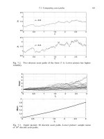
Figure 18.3 shows the value P
Am
(S, t) as a function of S, for t fixed. We
set E = 10, r = 0.06, σ = 0.3 and T = 1, and considered t = T/4. We used the
binomial method with a wide range of initial asset prices S
0
to compute values of
P
Am
(S, T/4). The figure shows that for small S the option value lies on the hockey
stick (S(t)), which is superimposed as a dashed line. For S bigger than some
level S

(T/4), the value P
Am
(S, T/4) lies above the hockey stick. It can also be
shown that the derivative ∂ P
Am
(S

(t), t)/∂ S =−1, so at the point S


(t) the curve
P
Am
(S(t), t) leaves the hockey stick smoothly, with a matching first derivative.
178 American options
100 150 200 250 300 350 400
0
0.002
0.004
0.006
0.008
0.01
M
Error in binomial method
100 200 400
10
−6
10
−4
10
−2
M
Error in binomial method
Fig. 18.2. Upper picture: Error in the binomial method for an American put as
the number of time points, M, increases from 100 to 400. Solid line is 1/M.
Lower picture: same data on a log–log scale.
0 2 4 6 8 10 12 14 16 18 20
0
1
2

3
4
5
6
7
8
9
10
t
=
T
/4
S
American put value
Fig. 18.3. Value P
Am
(S, T/4) for an American put, computed via the binomial
method. Hockey-stick payoff function (S) is superimposed as a dashed line.
18.5 Optimal exercise boundary 179
0 0.1 0.2 0.3 0.4 0.5 0.6 0.7 0.8 0.9 1
0
2
4
6
8
10
12
t
S
E

Exercise
Do not exercise
Fig. 18.4. Exercise boundary for an American put. Computed via the binomial
method.
Exercise 18.2 asks you to go half-way towards proving this, by establishing −1as
alower bound.
In Figure 18.4 we explicitly compute the optimal exercise boundary S

(t) for
the same E, r, σ and T as used in Figure 18.3. The boundary is shown as a solid
curve – below this curve it is optimal to exercise and above this curve it is op-
timal to hold on. At t = T/4wehaveS

(t) = 7.3, which agrees with the point
on the horizontal axis in Figure 18.3 where P
Am
(S, T/4) leaves the hockey stick.
We tracked the optimal exercise boundary by applying the binomial method with a
range of initial asset prices, S
0
.Ateach time point, t
i
,wedefined S

(t
i
) to be
the smallest value of S
i
n

over all binomial trees for which the e
−rδt
( pV
i+1
n+1
+
(1 − p)V
i+1
n
) term in (18.7) dominated the (S
i
n
) term. In other words, S

(t
i
)
was taken to be the smallest S
i
n
for which the binomial method chose not to
exercise.
It can be shown that Figure 18.4 is generic in the sense that
(i) S

(T ) = E,
(ii) S

(t) is a well-defined, single-valued function of t,
(iii) S


(t) is a nondecreasing function of t.
Exercise 18.3 deals with points (i) and (iii).
180 American options
18.6 Monte Carlo for an American put
We have seen that the binomial method has a natural extension from European to
American options. The same is not true for the Monte Carlo method. This mis-
match has two sources.
(a) Monte Carlo deals with single paths, whereas the binomial method essentially averages
over paths automatically.
(b) Monte Carlo works forward in time, whereas the binomial method runs backwards.
Monte Carlo for European options exploits the idea that the value can be ex-
pressed as an expectation. In the American case there is an analogous, but less
computationally useful, representation. Under the risk neutrality condition µ = r,
the time-zero American put value may be expressed as
P
Am
(S
0
, 0) = sup
0≤τ ≤T
E

e
−rτ
(S(τ))

, (18.8)
where τ is a stopping time.Todefine a stopping time precisely requires technic-
alities that have not been developed in this book, but the expression (18.8) can be

described informally as follows.
• The value taken by τ determines the time at which the option is exercised. So
e
−rτ
(S(τ )) in (18.8) represents the discounted payoff.
• The quantity τ is a random variable that depends upon the asset path S(t).
• Any rule that specifies τ as a function of the asset path S(t) can be used, with the proviso
that the decision to set τ = t

can only use information about S(t) for 0 ≤ t ≤ t

.
• The option value P
Am
(S
0
, 0) is given by using the rule for determining τ that leads to
the biggest expected payoff, suitably discounted for interest.
Putting this in words:
Imagine all possible exercise strategies, that is, all possible rules for determining when to
exercise the option. Suppose we judge the success of a strategy by its discounted expected
payoff. Then we recover the Black–Scholes American put option value if we use the best
out of all those exercise strategies that do not look forward in time – those that take an
exercise decision at each point in time using only information about the asset price up to
that time.
From a computational perspective, an enormous hurdle in (18.8) is the require-
ment to optimize over all allowable exercise strategies. It is impossible to write
down all such strategies in any useful way, let alone optimize over them! To
illustrate the idea, we restrict ourselves to a very simple class of allowable ex-
ercise strategies. Suppose we decide to exercise the option at time t if the dis-

counted payoff, e
−rt
(S(t)),exceeds some fixed level α>0. If we reach the ex-
piry date, T, and have not yet exercised the option, then it makes sense to exercise
if (S(T)) > 0. Overall, our exercise strategy may be written as follows.
18.6 Monte Carlo for an American put 181
0 1 2 3 4 5 6 7 8 9 10
0.8
0.9
1
1.1
1.2
1.3
1.4
1.5
α
Put value
American
European
Fig. 18.5. Asterisks are Monte Carlo approximations to the discounted expected
American put payoff with a simple exercise strategy parametrized by α. Upper
and lower horizontal lines show the true American and European values.
• Exercise at time t if e
−rt
[E − S(t)] >α.
• If we reach T, exercise if E − S(T)>0.
This is an allowable strategy, as the decision about whether to exercise at time t
uses only S(t).InFigure 18.5 we measure the success of this approach. Here we
valued an American option with S
0

= 9, E = 10, T = 1, r = 0.06 and σ = 0.3.
The Black–Scholes value, computed via the binomial method, was found to be
1.43. The corresponding European put option value is 1.32. These values are in-
dicated as horizontal lines. The asterisks in the figure show the Monte Carlo ap-
proximations to the option value, using the exercise strategy above, with a range of
choices for α. More precisely, we computed 10
6
risk-neutral discrete asset paths,
with a time spacing of δt = 10
−3
, and applied the strategy at each discrete time
point iδt. Confidence intervals for the sample means were smaller than the size of
the asterisks in the plot. We see from the figure that if α is taken to be around 2.5,
the discounted expected payoff is close to the Black–Scholes value. Exercise 18.4
asks you to explain the results for 0 ≤ α ≤ 1 and α large. In this example, we
are fortunate that optimizing over the parameter α in our simple class of exercise
strategies gives an answer that is close to the optimal over all allowable strate-
gies. Of course, if we were to change S
0
, E, T, r or σ then the optimal α would
182 American options
certainly change, and there is no guarantee that it would give a good approximation
to P
Am
(S
0
, 0).
In general, picking any particular allowable strategy and computing the dis-
counted expected payoff will lead to a lower bound on the true Black–Scholes
value.

By contrast, we could allow ourselves the luxury of peeking into the future in
order to select the best possible exercise times.
• Consider the whole path S(t) for 0 ≤ t ≤ T, and exercise where e
−rt
(S(t)) is
maximized.
For each asset path, this strategy does at least as well as the best allowable strategy.
Hence, the corresponding discounted expected payoff gives an upper bound on the
Black–Scholes value. In the example of Figure 18.5 the upper bound was 2.62,
which, as is typical, is too crude to be of much use.
18.7 Notes and references
Our derivation of the linear complementarity problem (18.2)–(18.6) followed
closely the treatment by Almgren (Almgren, 2002). It is possible to write the
American put valuation problem in terms of a PDE that explicitly involves the op-
timal exercise boundary, S

(t). This free boundary problem approach is described
in (Kwok, 1998; Wilmott et al., 1995), for example. Kwok (Kwok, 1998) gives
examples of more complex options with early exercise features for which the ex-
ercise and non-exercise regions are made up of disconnected sets. The condition
that ∂ P
Am
(S

(t), t)/∂ S =−1, which we illustrated in Figure 18.3, is discussed in
detail in (Kwok, 1998) and (Wilmott et al., 1995).
Convergence of the binomial method for American options is treated in (Leisen,
1998), where an error bound of the form (16.8) is derived.
The argument in Section 18.2 that shows the equivalence of European and
American call values fails to hold when the asset pays dividends, see (Hull,

2000; Kwok, 1998; Wilmott et al., 1995), for example, for details of how the theory
can be adapted.
Applied mathematicians have recently become interested in the nature of the
optimal exercise boundary for t ≈ T.Itcan be shown that as the boundary S

(t)
approaches E as t → T
−
, its tangent becomes unbounded, as may be observed in
Figure 18.4. The precise nature of this singularity is explored in (Goodman and
Ostrov, 2002; Kuske and Keller, 1998), for example.
Bj
¨
ork (Bj
¨
ork, 1998) is a good source for the mathematics behind (18.8).
Until quite recently, most researchers believed that a Monte Carlo approach
could not be used for valuing American options. However, a number of authors
18.8 Program of Chapter 18 and walkthrough 183
now argue that, with appropriate extensions, competitive Monte Carlo based com-
putational algorithms are achievable; see (Anderson and Broadie, 2001; Boyle
et al., 1997; Fu et al., 2001; Longstaff and Schwartz, 2001; Rogers, 2002), for
example.
EXERCISES
18.1. Repeat the analysis in Section 18.3 for the case of an American call
option. Show that the Black–Scholes European call option formula (8.19)
satisfies the relevant analogues of (18.2)–(18.6). Deduce that an American
call option has the same value as the corresponding European call option.
18.2.  In Section 18.5 it was mentioned that ∂ P
Am

(S

(t), t)/∂ S =−1. Give a
simple explanation why ∂ P
Am
(S

(t), t)/∂ S cannot be less that −1.
18.3.  Given that there is a well-defined, single-valued optimal exercise
boundary function S

(t) for an American put, show that S

(T) = E and
that S

(t) is a nondecreasing function of t.
18.4.  Explain the behaviour of the Monte Carlo approximations in Figure 18.5
for 0 ≤ α ≤ 1 and α large.
18.5.  Which of the following exercise strategies are allowable in (18.8)?
Strategy 1:
• Exercise at time t if S(t)<
1
2
E.
• If we reach T, exercise if E − S(T)>0.
Strategy 2:
• Exercise at time t if S(t)<min(E, 1.1 min
0≤r≤T
S(r)).

• If we reach T, exercise if E − S(T)>0.
Strategy 3:
• Exercise at time t if S(t)<min(E,
1
2
min
0≤r≤t/2
S(r)).
• If we reach T, exercise if E − S(T)>0.
18.8 Program of Chapter 18 and walkthrough
In ch18, listed in Figure 18.6, we give a modified version of ch16 that values an American
put with the binomial method. After initializing parameters, we create the one-dimensional
array dpowers with entries d
M
, d
M−1
, ,d
0
and the one-dimensional array upowers with entries
u
0
, u
1
, ,u
M
.Itfollows that S*dpowers.*upowers gives the asset values S
M
0
, S
M

1
, ,S
M
M
at
expiry in the asset price tree of Figure 16.1, and
S*dpowers(M-i+2:M+1).*upowers(1:i);
184 American options
%CH18 Program for Chapter 18
%
% Implements binomial method for an American put.
%%%%%% Problem and method parameters %%%%%%%%%
S=3;E=4;T=1;r=0.05; sigma = 0.3;
M=400; dt = T/M; p =0.5;
u=exp(sigma*sqrt(dt) + (r-0.5*sigmaˆ2)*dt);
d=exp(-sigma*sqrt(dt) + (r-0.5*sigmaˆ2)*dt);
%%%%%%%%%%%%%%%%%%%%%%%%%%%%%%%%%%
% Initial computations
dpowers = d.ˆ([M:-1:0]’);
upowers = u.ˆ([0:M]’);
%Time T option values
W=max(E-S*dpowers.*upowers,0);
%Work back to option value at time zero
for i = M:-1:1
Si = S*dpowers(M-i+2:M+1).*upowers(1:i);
W=max(max(E-Si,0),exp(-r*dt)*(p*W(2:i+1)+(1-p)*W(1:i)));
end
disp(’Option value is’), disp(W)
Fig. 18.6. Program of Chapter 18: ch18.m.
gives the asset values S

i
0
, S
i
1
, ,S
i
i
at the ith time level. In this way, the iteration (18.7) is enscap-
sulated as
W=max(max(E-Si,0),exp(-r*dt)*(p*W(2:i+1)+(1-p)*W(1:i)));
As with ch16, the loops exits with a scalar value for W that gives the option value V
0
0
.
The option value output by ch18.m is 1.0158. The validity of the result will be confirmed by
ch24 in Chapter 24.
PROGRAMMING EXERCISES
P18.1. Alter ch18 in order to re-create Figure 18.4.
P18.2. Think up an allowable exercise strategy and test it in the manner of
Figure 18.5.
Quotes
Although simulation is a powerful tool
for solving some higher-dimensional problems,
18.8 Program of Chapter 18 and walkthrough 185
conventional wisdom was that
simulation could not be applied to American-style pricing problems.
The algorithms described here represent the first attempts to solve these problems
that were long thought to be computationally intractable.
PHELIM BOYLE, MARK BROADIE AND PAUL GLASSERMAN (Boyle et al., 1997)

Academia was teeming with nerdy mathematicians who had been publishing
unintelligible dissertations on markets for years.
Wall Street had started to hire them, but only for research,
where they’d be out of harm’s way.
On Wall Street, the eggheads were stigmatized as ‘quants’,
unfit for the man’s game of trading.
ROGER LOWENSTEIN (Lowenstein, 2001)
I prefer the judgement of a 55-year old trader
to that of a 25-year old mathematician.
ALAN GREENSPAN,source (Taleb, 1997)

19
Exotic options
OUTLINE
• European-style options
• path-dependent options: lookbacks, barriers and Asians
• early exercise options: Bermudans and shouts
• Monte Carlo and binomial methods
19.1 Motivation
So far, we have seen European options and American-style options. A bewildering
array of alternatives are also available; these go by the general name of exotic
options. Each type of option is distinguished by
(i) the nature of its path dependency – the way in which the payoff depends upon the asset
path S(t) for 0 ≤ t ≤ T , and
(ii) whether early exercise is allowed.
In many cases, exact expressions for the option value are not available, and hence
approximations must be computed. This chapter introduces some of the less eso-
teric exotics and discusses the use of our two computational algorithms: the bino-
mial and Monte Carlo methods. A third computational approach, numerical solu-
tion of a Black–Scholes PDE formulation, is covered in Chapters 23 and 24.

19.2 Barrier options
Barrier options have a payoff that switches on or off depending on whether the
asset crosses a pre-defined level.
• A down-and-out call option has a payoff that is zero if the asset crosses some pre-
defined barrier B < S
0
at some time in [0, T ]. If the barrier is not crossed then the
payoff becomes that of a European call, max(S(T ) − E, 0).
187
188 Exotic options
0
T
B
E
Time
Asset
Fig. 19.1. Two asset paths and a barrier, B. The thicker asset path crosses the
barrier and hence would give zero payoff in a down-and-out call. The thinner asset
path fails to cross the barrier and hence would give zero payoff in a down-and-in
call.
• A down-and-in call option has a payoff that is zero unless the asset crosses some pre-
defined barrier B < S
0
at some time in [0, T ]. If the barrier is crossed then the payoff
becomes that of a European call, max(S(T ) − E, 0).
One reason for the popularity of barrier options is that, because the payoff op-
portunities are more limited, they are cheaper to buy than Europeans. Figure 19.1
illustrates the idea. Here, two asset paths are shown. Both expire above the ex-
ercise price: S(T )>E. Despite finishing the higher, the thicker of the two paths
dips lower, crossing the barrier. The thicker path would give a nonzero payoff for a

down-and-in call, but a zero payoff for a down-and-out call. Conversely, the thin-
ner path would give a zero payoff for a down-and-in call, but a nonzero payoff for
adown-and-out call.
The hedging idea from Chapter 8 remains valid for barrier options. Let C
B
(S, t)
denote the value of a down-and-out call option at asset price S and time t. The
Black–Scholes PDE (8.15) is relevant unless the barrier is crossed, so C
B
(S, t)
must satisfy the PDE on the domain 0 ≤ t ≤ T , B ≤ S.IfS = B then the option
becomes worthless, giving
C
B
(B, t) = 0, for 0 ≤ t ≤ T. (19.1)
19.2 Barrier options 189
0
B E
S
Call value
Down-and-out
European
Fig. 19.2. Time-zero down-and-out call value (19.3) as a function of S.
Also, at expiry, for S(T )>B we must recover the European value, so
C
B
(S, T ) = C(S, T ), for B ≤ S. (19.2)
Here, C(S, t) denotes the European value (8.19). In the case B < E it can be
shown that a solution to the Black–Scholes PDE on the domain 0 ≤ t ≤ T , B ≤ S,
that satisfies (19.1) and (19.2) is given by

C
B
(S, t) = C(S, t) −
(
S/B
)
1−2r/σ
2
C(B
2
/S, t); (19.3)
see Exercise 19.2.
We note that (19.3) immediately confirms that the down-and-out call is worth
less than the European call.
A plot of the time-zero value C
B
(S, 0) in (19.3) for B < E is given in
Figure 19.2. The European value is also shown. As we would expect, as the initial
asset price increases, and so the probability of hitting the barrier decreases, the
down-and-out call value approaches that of the European.
Given a formula for a down-and-out call, the corresponding down-and-in can
be found from the relation
in + out = European, (19.4)
see Exercise 19.3.
190 Exotic options
Replacing ‘down’ by ‘up’ gives another class of barrier options.
• An up-and-out call option has a payoff that is zero if the asset crosses some pre-defined
barrier B > S
0
at some time in [0, T ]. If the barrier is not crossed then the payoff be-

comes that of a European call, max(S(T ) − E, 0).
• An up-and-in call option has a payoff that is zero unless the asset crosses some pre-
defined barrier B > S
0
at some time in [0, T ]. If the barrier is crossed then the payoff
becomes that of a European call, max(S(T ) − E, 0).
There are also, of course, put versions of the above calls; just replace the word
‘call’ by ‘put’ in each case. This gives a total of eight different up/down-and-in/out
calls/puts. In each case, an analytical formula for the option value can be obtained
by solving the Black–Scholes PDE with appropriate final time and boundary con-
ditions. Formulas for each type of barrier option can be found via the references
in Section 19.7. As an example that we will return to in Section 19.6, we give the
formula for an up-and-out call:
S

N (d
1
) − N(e
1
) −

B
S

1+2r/σ
2
(N( f
2
) − N(g
2

))

−Ee
−r(T −t)

N (d
2
) − N(e
2
) −

B
S

−1+2r/σ
2
(N( f
1
) − N(g
1
))

. (19.5)
Here, d
1
and d
2
are defined in (8.20) and (8.21) and
e
1

=
log(S/B) +(r +
1
2
σ
2
)(T − t)
σ
√
T − t
,
e
2
=
log(S/B) +(r −
1
2
σ
2
)(T − t)
σ
√
T − t
,
f
1
=
log(S/B) −(r −
1
2

σ
2
)(T − t)
σ
√
T − t
,
f
2
=
log(S/B) −(r +
1
2
σ
2
)(T − t)
σ
√
T − t
,
g
1
=
log(SE/B
2
) − (r −
1
2
σ
2

)(T − t)
σ
√
T − t
,
g
2
=
log(SE/B
2
) − (r +
1
2
σ
2
)(T − t)
σ
√
T − t
.
Figure 19.3 plots the up-and-out call value (19.5) at time zero, along with the
corresponding European. The picture illustrates that barrier options can be signif-
icantly cheaper than Europeans. The up-and-out call has a limited up-side – the
19.3 Lookback options 191
0
E B
S
Call value
Up–and–out
European

Fig. 19.3. Time-zero up-and-out call value (19.5) as a function of S.
payoff cannot exceed B − E,and hence can be bought for much less than the
European version.
There are many generalizations of those eight basic barrier options.
• Double barrier options impose upper and lower bounds on the asset price, and payoff
may knock in (or out) if either barrier is (or both barriers are) crossed.
• Partial barrier options have barriers that apply for a limited time interval.
• Parisian options have barriers that must remain crossed for some pre-specified amount
of time.
• More generally, the barrier may be time-dependent and the nature of the option may be
re-set (e.g. to another barrier option) if a barrier is crossed.
Although the Black–Scholes analysis remains relevant in all cases, the more com-
plicated barrier options do not admit analytical expressions for the value.
19.3 Lookback options
The payoff for a lookback option depends upon either the maximum or the mini-
mum value attained by the asset. There are two broad categories, fixed and floating
strikes. In describing them, we use the notation
S
max
:= max
[0,T ]
S(t) and S
min
:= min
[0,T ]
S(t)
192 Exotic options
to denote the extreme asset values.
• A fixed strike lookback call option has payoff at the expiry date T given by max(S
max

−
E, 0).
• A fixed strike lookback put option has payoff at the expiry date T given by max(E −
S
min
, 0).
• A floating strike lookback call option has payoff at the expiry date T given by S(T ) −
S
min
.
• A floating strike lookback put option has payoff at the expiry date T given by S
max
−
S(T ).
These lookback options are clearly more valuable than the corresponding Euro-
peans. The fixed strike lookbacks differ from European options in that the final
asset value S(T ) is replaced by the ‘best’ asset price – the maximum in the case
of a call and the minimum in the case of a put. With a floating strike, the exercise
(strike) price becomes the extremely favourable minimum asset price for a call and
maximum asset price for a put. In the floating case it will always be worthwhile to
exercise, so the word ‘option’ is perhaps inappropriate.
It is possible to derive Black–Scholes formulas for the four lookback cases
above, see Section 19.7 for references. There are many extensions of these ideas,
typically designed to offer some of the lookback desirability at a cheaper price;
for example by looking back over a limited time period or over a finite number of
points in time. In many cases, the options may only be valued by computational
means.
19.4 Asian options
Whereas barriers and lookbacks focus on extreme values of the asset, Asian op-
tions are determined by average case behaviour.

• An average price Asian call option has payoff at the expiry date T given by
max

1
T

T
0
S(τ )dτ − E, 0

.
• An average price Asian put option has payoff at the expiry date T given by
max

E −
1
T

T
0
S(τ )dτ, 0

.
Here we are replacing the final asset price S(T ) that would be used in a European
option by the average asset price over the time period.
• An average strike Asian call option has payoff at the expiry date T given by
max

S(T ) −
1

T

T
0
S(τ )dτ, 0

.
19.5 Bermudan and shout options 193
• An average strike Asian put option has payoff at the expiry date T given by
max

1
T

T
0
S(τ )dτ − S(T ), 0

.
Here we are replacing the strike, or exercise, price E , that would be used in a
European option, by the average asset price.
Other Asian options can be defined, for instance, by replacing the continuous
average

T
0
S(τ )dτ/T by an arithmetic average
1
n
n


i=1
S(t
i
),
or geometric average

n

i=1
S(t
i
)

1/n
,
over n time points, 0 ≤ t
1
< t
2
< ···< t
n
≤ T .(In practice, as the real asset price
does not change continuously, even the continuous average would have to be ap-
proximated from discrete market data.)
The path dependency for Asians is, in a sense, more complicated than that for
barrier and lookback options. The payoff depends on the range of asset prices, not
just the extremes. It is possible to accommodate Asian options into the Black–
Scholes framework, but exact solutions have been found only in certain cases. One
such case is treated in Exercise 19.6.

19.5 Bermudan and shout options
A Bermudan option differs from the corresponding American option in only one
respect. While the American option allows the holder to exercise at any time in
[0, T ], the Bermudan option restricts the early exercise facility to a fixed number
of pre-determined dates.
As in the American case, there is no general analytical formula for the Bermu-
dan option value.
The simplest version of a shout call option allows the holder to ‘shout’ at most
once to the writer between times 0 and T . The payoff at expiry is given by

max(S(T ) − E, S(τ ) − E), if holder shouted at time τ,
max(S(T ) − E, 0), if holder did not shout,

(19.6)
and we may make the perfectly sensible assumption that a shout will only take
place if S(τ ) > E. The effect of shouting is to lock in a payoff of at least S(τ ) − E;
the actual payoff will then be the maximum of this value and the European payoff.
Typically, a shout will take place if the holder feels that the asset price has peaked
194 Exotic options
and is about to plummet. As with Americans and Bermudans, there is no exact
valuation formula for shouts.
19.6 Monte Carlo and binomial for exotics
The Monte Carlo method that we described in Chapter 15 extends easily to handle
path dependency. The extra step required is to set up a grid of points t
j
= jt, for
0 ≤ j ≤ N , where N is a large number and t = T /N.Wearegiven S(0) = S
0
,
so from (6.9) we can compute an asset price S(t

j+1
) in terms of S(t
j
) using the
formula
S(t
j+1
) = S(t
j
)e
(r−
1
2
σ
2
)t+σ
√
tZ
j
, for i.i.d. Z
j
∼ N(0, 1). (19.7)
(Note that we use the risk neutrality assumption, µ = r .) This gives us the asset
price at a closely spaced set of points in [0, T ], so we can compute approxima-
tions to the max, min or integral, and test for barrier crossings. For example, the
following algorithm values an up-and-out call option. Here, M is the number of
asset paths that we sample.
for i =1toM
for j =0toN − 1
compute an N(0, 1) sample ξ

j
set S
j+1
= S
j
e
(r−
1
2
σ
2
)t+σ
√
tξ
j
end
set S
max
i
= max
0≤j≤N
S
j
if S
max
i
< B set V
i
= e
−rT

max(S
N
− E, 0), otherwise set V
i
= 0
end
set a
M
=
1
M

M
i=1
V
i
set b
2
M
=
1
M−1

M
i=1
(V
i
− a
M
)

2
The result gives an approximate option price a
M
and an approximate 95% confi-
dence interval (15.5).
For Asian options we could use the Riemann sum t

N
j=1
S
j
to approximate
the integral

T
0
S(τ )dτ .With an average price Asian put this would give the fol-
lowing algorithm:
for i =1toM
for j =0toN − 1
compute an N(0, 1) sample ξ
j
set S
j+1
= S
j
e
(r−
1
2

σ
2
)t+σ
√
tξ
j
end
set Smean
i
= t

N
j=1
S
j
19.6 Monte Carlo and binomial for exotics 195
Table 19.1. Ninety-five per cent confidence intervals for Monte Carlo
on a European up-and-out call. Black–Scholes value (19.5) is 0.0983
t = 10
−2
t = 10
−3
t = 10
−4
M = 10
2
[0.0469, 0.1671] [0.0397, 0.1387] [0.0569, 0.1813]
M = 10
3
[0.0961, 0.1347] [0.0756, 0.1104] [0.0726, 0.1046]

M = 10
4
[0.1042, 0.1163] [0.0997, 0.1112] [0.0926, 0.1038]
M = 10
5
[0.1097, 0.1136] [0.1000, 0.1036] [0.0981, 0.1071]
set V
i
= e
−rT
(E − Smean
i
, 0)
end
set a
M
=
1
M

M
i=1
V
i
set b
2
M
=
1
(M−1)


M
i=1
(V
i
− a
M
)
2
Computational example We now apply Monte Carlo to the task of valuing
an up-and-out call with S
0
= 5, E = 6, σ = 0.3, r = 0.05 and T = 1, with
barrier B = 8. The Black–Scholes value (19.5) was found to be 0.0983. Ta-
ble 19.1 shows the 95% confidence intervals for timesteps t of 10
−2
,10
−3
and 10
−4
(so N = 10
2
,10
3
and 10
4
), and number of discrete sample paths M
equal to 10
2
,10

3
,10
4
and 10
5
.Asthe theory predicts, increasing M causes the
confidence interval to shrink. However, in general the Monte Carlo method is
over-estimating the option value. In particular, even for the largest sample size,
M = 10
5
, the t = 10
−2
and t = 10
−3
confidence intervals do not contain
the Black–Scholes value. To understand why, recall that the method is sampling
the path at finitely many discrete points, rather than over the continuous inter-
val [0, T ]. Because the discrete test max
0≤j≤N
S
j
< B is less stringent than
the continuous test max
0≤t≤T
S(t)<B, the Monte Carlo method allows more
nonzero payoffs than it should. As t is refined (so N increases) the discrete
test approaches the continuous one, and the bias becomes less pronounced. In
Table 19.1, we see that for t = 10
−4
and M = 10

5
, the confidence interval
does contain the Black–Scholes value, although it is still skewed to the right. A
more expensive simulation with t = 10
−5
and M = 10
6
improved the confi-
dence interval to [0.0980, 0.0992]. ♦
Although the Monte Carlo method typically produces low-accuracy solutions,
it does have the benefit of flexibility. It should be clear that the pathwise sampling
approach can be applied to any of the generalized path-dependent options men-
tioned in Sections 19.2, 19.3, 19.4.
196 Exotic options
The binomial method does not naturally extend to path-dependent options, as
the basic recombining tree of asset prices in Figure 16.1 loses track of individual
asset paths. At time t
M
= T we have only a set of asset prices {S
M
n
}
M
n=0
and no
information about how those asset prices were reached. (In fact we are essentially
averaging over all paths that finished at that price). Even so, researchers have de-
veloped techniques for adapting the binomial method to barriers, lookbacks and
Asians; see Section 19.7 for references.
Conversely, as we have seen in Chapter 18, early exercise does not fit comfort-

ably with Monte Carlo, but is easily incorporated into the binomial method.
In the case of Bermudan options, it is clear that the binomial method may be
used. In fact, as applied to American options in Section 18.4, the method is really
approximating the American by a Bermudan with a large number of closely spaced
early exercise points. Bermudan options can thus be handled this way if we simply
make sure that the prescribed exercise dates are included in the set of times t
i
, and
then use (18.7) if t
i
is an allowable exercise time and (16.3) otherwise.
To handle the shout option with payoff (19.6), note that if a shout happened at
time τ ,then the payoff may be written
max
(
S(T ) − S(τ ), 0
)
+ S(τ) − E. (19.8)
From this point of view, a shout locks in a bonus of S(τ) − E and moves the
exercise price to S(τ). Once τ and S(τ) are known, the first term in (19.8),
max(S(T ) − S(τ ), 0), corresponds to the payoff for a European option, so it is
given by the Black–Scholes formula (8.19) with time set to τ and exercise price
set to S(τ ).Wemay thus use the approach outlined in Section 18.4 with (18.7)
replaced by
V
i
n
= max

value (19.8) from shouting at (t

i
, S
i
n
),
e
−rδt

pV
i+1
n+1
+ (1 − p)V
i+1
n

, (19.9)
for 0 ≤ n ≤ i and 0 ≤ i ≤ M −1. The overall method is then defined by (16.1),
(16.2) and (19.9).
19.7 Notes and references
The texts (Kwok, 1998) and (Wilmott et al., 1995), and any of the Wilmott
incarnations, such as (Wilmott, 1998), give much more detail about how the
Black–Scholes PDE framework can be used to value exotic options. Also (Hull,
2000; Kwok, 1998; Wilmott, 1998) are good sources for analytical valuation for-
mulas.