An Introduction to Financial Option Valuation Mathematics Stochastics and Computation_11 doc

21.5 Analysis of the uniform case 219
Table 21.1. Ninety-five per cent confidence intervals for (21.4) and
(21.6) on problem (21.3), plus ratios of their widths
M Standard Antithetic Ratio of widths
10
2
[1.8841, 2.0752] [1.9875, 2.0012] 14.0
10
3
[1.9538, 2.0087] [1.9976, 2.0017] 13.4
10
4
[1.9890, 2.0062] [1.9997, 2.0010] 13.5
10
5
[1.9969, 2.0023] [1.9998, 2.0002] 13.5
of the two confidence intervals. This is precisely the ratio of the square roots
of the sample variances. As predicted by (21.11), it converges to
√
181.2485 ≈
13.5. As a practical note, it is worth emphasizing that the confidence intervals
for the antithetic variates estimate were computed via the sample variance of
{

Y
i
}
M
i=1
, which are independent, and not


e
√
U
i

M
i=1
∪

e
√
1−U
i

M
i=1
, which are
highly correlated. ♦
21.5 Analysis of the uniform case
To understand how the antithetic variate technique works, consider the more gen-
eral case of approximating
I =
E( f (U )), where U ∼ U(0, 1),
for some function f . The standard Monte Carlo estimate is
I
M
=
1
M
M


i=1
f (U
i
), with i.i.d. U
i
∼ U(0, 1), (21.12)
and the antithetic alternative is

I
M
=
1
M
M

i=1
f (U
i
) + f (1 −U
i
)
2
, with i.i.d. U
i
∼ U(0, 1). (21.13)
Copying the way that we derived (21.8), we find that
var

f (U

i
) + f (1 −U
i
)
2

=
1
2
(
var
(
f (U
i
)
)
+ cov
(
f (U
i
), f (1 −U
i
)
))
.
(21.14)
The success of the new scheme hinges on whether var

1
2

( f (U
i
)+
f (1 −U
i
))

is smaller than var( f (U
i
)). The identity (21.14) tells us that effi-
ciency boils down to making cov
(
f (U
i
), f (1 −U
i
)
)
as negative as possible.We
want f (U
i
) to be big (relative to its mean) when f (1 − U
i
) is small (relative to
its mean). Intuitively, this approach will work when f is monotonic. Loosely, the
220 Monte Carlo Part II: variance reduction by antithetic variates
antithetic variate technique attempts to compensate for samples that are above the
mean by adding samples that are below the mean, and vice versa.
We may convert this intuition into a mathematical result. First we recall that
to say a function f is monotonic increasing means x

1
≤ x
2
⇒ f (x
1
) ≤ f (x
2
).
Similarly, to say a function f is monotonic decreasing means x
1
≤ x
2
⇒ f (x
1
) ≥
f (x
2
).Itfollows straightforwardly that if f and g are both monotonic increasing
functions or both monotonic decreasing functions then
(
f (x) − f (y)
)(
g(x) − g(y)
)
≥ 0, for any x and y, (21.15)
see Exercise 21.5. Now we prove a useful lemma.
Lemma If f and g are both monotonic increasing functions or both monotonic
decreasing functions then, for any random variable X ,
cov( f (X), g(X)) ≥ 0.
Proof Let Y be a random variable that is independent of X with the same

distribution. From (21.15) we may write
(
f (X) − f (Y )
)(
g(X) − g(Y )
)
≥ 0.
So the random variable
(
f (X) − f (Y )
)(
g(X) − g(Y )
)
must have a non-
negative expected value. Hence
0 ≤
E
[
(
f (X) − f (Y )
)(
g(X) − g(Y )
)
]
=
E
[
f (X)g(X)
]
−

E
[
f (X)g(Y )
]
−
E
[
f (Y )g(X)
]
+
E
[
f (Y )g(Y )
]
.
Since X and Y are i.i.d., that last right-hand side simplifies to
2
E
[
f (X)g(X)
]
− 2
E
[
f (X)
]
E
[
g(X)
]

,
which is 2 cov( f (X), g(X)), and the result follows. ♦
Now note that if f is a monotonic increasing function, then so is −f (1 − x).
Similarly, if f is a monotonic decreasing function, then so is − f (1 − x).Inei-
ther case, applying our lemma gives cov( f (X), −f (1 − X)) ≥ 0. Equivalently,
cov( f (X), f (1 − X)) ≤ 0. In (21.14) this shows that
var

f (U
i
) + f (1 −U
i
)
2

≤
1
2
var
(
f (U
i
)
)
, (21.16)
21.6 Normal case 221
when f is monotonic. In words:
For monotonic f , the variance in the antithetic sample is always less than or equal to half
that in the standard sample.
Of course, this is only a bound. The actual improvement can be much better, as in

the f (x) = e
√
x
example of the previous section.
21.6 Normal case
The antithetic variates trick is not restricted to functions of uniform random vari-
ables. In the case of
I =
E( f (U )), where U ∼ N(0, 1), (21.17)
the standard Monte Carlo estimate is
I
M
=
1
M
M

i=1
f (U
i
), with i.i.d. U
i
∼ N(0, 1), (21.18)
and the antithetic alternative is

I
M
=
1
M

M

i=1
f (U
i
) + f (−U
i
)
2
, with i.i.d. U
i
∼ N(0, 1). (21.19)
Because the N(0, 1) distribution is symmetric about the origin, rather than about
1
2
, the antithetic estimate uses −U
i
, rather than 1 −U
i
.Ofcourse, −U
i
is also an
N(0, 1) random variable.
The above analysis that gave us (21.16) can then be repeated to give us
var

f (U
i
) + f (−U
i

)
2

≤
1
2
var
(
f (U
i
)
)
(21.20)
when f is monotonic.
Computational example Here we show the antithetic variate trick in use with
N(0, 1) samples. We take (21.17) with f (x) = (1/
√
e)e
x
,sothat E( f (U )) = 1
(see Exercise 15.3). (A similar computation was done in Chapter 15 for standard
Monte Carlo. We now scale by 1/
√
e so that the confidence intervals are easier
to assimilate.) Table 21.2 shows the 95% confidence intervals for (21.18) and
(21.19). As in the previous example, we took M = 10
2
, 10
3
, 10

4
, 10
5
, and used
the same random number samples for the two methods. The antithetic version
gives almost twice as much accuracy. ♦
222 Monte Carlo Part II: variance reduction by antithetic variates
Table 21.2. Ninety-five per cent confidence intervals for (21.18) and
(21.19) on problem (21.17) with f (x) = (1/
√
e)e
x
, plus ratios of
their widths
M Standard Antithetic Ratio of widths
10
2
[0.8247, 1.2819] [0.9518, 1.6767] 0.6
10
3
[0.9713, 1.1574] [1.0166, 1.1244] 1.7
10
4
[0.9647, 1.0137] [0.9945, 1.0243] 1.6
10
5
[0.9953, 1.0115] [0.9955, 1.0046] 1.8
21.7 Multivariate case
The antithetic variates idea extends readily to the case where f is a function of
more than one random variable. For example, suppose we wish to approximate

I =
E( f (U, V, W)), where U, V, W are i.i.d. ∼ N(0, 1).
The standard Monte Carlo estimate is
I
M
=
1
M
M

i=1
f (U
i
, V
i
, W
i
), with U
i
, V
i
, W
i
i.i.d. ∼ N(0, 1),
and the antithetic version is

I
M
=
1

M
M

i=1
f (U
i
, V
i
, W
i
) + f (−U
i
, −V
i
, −W
i
)
2
,
with U
i
, V
i
, W
i
i.i.d. ∼ N(0, 1).
An extension of the above analysis shows that benefits accrue when f is monotonic
in each of the arguments.
21.8 Antithetic variates in option valuation
The application that we have in mind is, of course, Monte Carlo estimation of

path-dependent exotic options. In this case we discretize the time interval [0, T ]
and compute risk-neutral asset prices at {t
i
}
N
i=1
, with t
i
= i t, N t = T .We
know that on each increment the price update uses an N(0, 1) random variable
Z
j
coming from the i.i.d. sequence {Z
0
, Z
1
, ,Z
N −1
} according to (19.7). We
wish to compute the expected value of some payoff function. We are therefore
looking for the expected value of a function of the N i.i.d. N(0, 1) random vari-
ables {Z
0
, Z
1
, ,Z
N −1
}. The antithetic variates technique is to take the average
payoff from one path with samples {Z
0

, Z
1
, ,Z
N −1
} and another path with
21.8 Antithetic variates in option valuation 223
0
T
Time
Asset
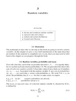
Fig. 21.1. A pair of discrete asset paths computed using antithetic variates. The
payoff from both paths is averaged in order to give a single sample.
samples {−Z
0
, −Z
1
, ,−Z
N −1
}. Where one path zig-zags, the other path zag-
zigs. Figure 21.1 illustrates such a pair of paths.
Computational example We value an up-and-in call option with S
0
= 5, E =
6, r = 0.05, σ = 0.3 and T = 1, using a timestep t = 10
−4
,soN = 10
4
.We
take B = 8 for the barrier level. Recall from Section 19.2 that
• the payoff is zero if the asset never attained the price B,that is, if max

[0,T ]
S(t)<
B,
• the payoff is equal to the European call value max(S(T ) − E, 0) if the asset at-
tained the price B, that is, if max
[0,T ]
S(t) ≥ B.
Using the ideas from Section 19.6, a basic Monte Carlo strategy can be sum-
marized as follows:
for i = 1toM
for j = 0toN − 1
compute an N(0, 1) sample ξ
j
set S
j+1
= S
j
e
(r−
1
2
σ
2
)t+σ
√
tξ
j
end
set S
max

i
= max
0≤j ≤N
S
j
if S
max
i
> B set V
i
= e
−rT
max(S
N
− E, 0), otherwise V
i
= 0
224 Monte Carlo Part II: variance reduction by antithetic variates
end
set a
M
=

1
M


M
i=1
V

i
set b
2
M
=

1
M−1


M
i=1
(V
i
− a
M
)
2
This gives an approximate option price a
M
and an approximate 95% confi-
dence interval (15.5).
The corresponding antithetic variate version is
for i = 1toM
for j = 0toN − 1
compute an N(0, 1) sample ξ
j
set S
j+1
= S

j
e
(r−
1
2
σ
2
)t+σ
√
tξ
j
set S
j+1
= S
j
e
(r−
1
2
σ
2
)t−σ
√
tξ
j
end
set S
max
i
= max

0≤j ≤N
S
j
set S
max
i
= max
0≤j ≤N
S
j
if S
max
i
> B set V
i
= e
−rT
max(S
N
− E, 0), otherwise V
i
= 0
if
S
i
max
> B set V
i
= e
−rT

max(S
N
− E, 0), otherwise V
i
= 0
set

V
i
=
1
2
(V
i
+ V
i
)
end
set a
M
=
1
M

M
i=1

V
i
set b

2
M
=
1
M−1

M
i=1
(

V
i
− a
M
)
2
Table 21.3 shows the 95% confidence intervals, and the ratios of their widths,
for M = 10
2
, 10
3
, 10
4
, 10
5
.Wesee that using antithetic variates shrinks the con-
fidence intervals by a factor of around 1.5. As mentioned in Section 19.6, the
overall accuracy of the process depends not only on the error in the Monte Carlo
approximation to the mean, but also on the error arising from the time discretiza-
tion – we take the maximum over a discrete set of points rather than over a con-

tinuous time interval. In this experiment we found that using smaller t values
did not significantly change the computed results, so the sampling error is dom-
inant. ♦
Table 21.3. Ninety-five per cent confidence intervals, plus ratios of their
widths, for standard and antithetic Monte Carlo on an up-and-in call
M Standard Antithetic Ratio of widths
10
2
[0.0878, 0.3219] [0.1239, 0.3061] 1.3
10
3
[0.2285, 0.3333] [0.2238, 0.2936] 1.5
10
4
[0.2443, 0.2764] [0.2370, 0.2580] 1.5
10
5
[0.2359, 0.2458] [0.2373, 0.2440] 1.5
21.10 Program of Chapter 21 and walkthrough 225
21.9 Notes and references
The texts (Hammersley and Handscombe, 1964; Madras, 2002; Ripley, 1987) that
we mentioned in Chapter 15 are good sources of general information about an-
tithetic variates, and (Boyle et al., 1997; Boyle, 1977; Clewlow and Strickland,
1998; J
¨
ackel, 2002) look at practical issues for option valuation.
EXERCISES
21.1.  Show that (21.1) and (21.2) are equivalent and hence conclude that if X
and Y are independent then cov(X, Y ) = 0.
21.2.  Show that I = 2in(21.3) and confirm (21.5).

21.3.  Establish the identity (21.7). [Hints: make use of (3.6) and (3.10) in
(21.1).]
21.4.  Use your favourite scientific computation package to confirm that
var(

Y
i
) ≈ 0.001073 in (21.10). (For example, a suitable approxima-
tion to the integral

1
0
e
√
x+
√
1−x
dx in (21.10) can be obtained from
>> quadl(’exp(sqrt(x) + sqrt(1-x))’,0,1,1e-9) in MATLAB.)
21.5.  Prove the statement involving (21.15).
21.6.  Consider the case where f is a monotonic increasing function that is
extremely expensive to evaluate on a computer – so much so that the cost
of a sample from a pseudo-random number generator is negligible by com-
parison. Can we still argue that the antithetic variate estimate (21.13) is at
least as efficient as the standard one, (21.12)?
21.7.  Show that the antithetic estimators (21.13) and (21.19) are exact in the
case where f is linear, that is, f (x) = αx + β, for α, β ∈
R.What can you
say about the corresponding confidence intervals?
21.8. Find a simple example where antithetic variates are less efficient than

standard Monte Carlo.
21.10 Program of Chapter 21 and walkthrough
In ch21, listed in Figure 21.2, we value an up-and-out call option. We use the same parameters as for
ch19,soweknow that the Black–Scholes value is 0.1857.
The first part of the for loop implements standard Monte Carlo, as in ch19.Wethen compute
the payoffs with a negated version of the pseudo-random numbers in samples. The ith entry of the
array Vanti thus contains the average of the payoffs for the ith asset path and its antithetic twin.
Running ch21 gives conf = [0.1763, 0.1937] for the Monte Carlo confidence interval. This
is identical to the interval produced by ch19, because by setting the random number generator to
the same state with randn(’state’,100),weare using exactly the same samples. The antithetic
version gives confanti = [0.1807, 0.1921], which is roughly 1.5 times as small as the standard
Monte Carlo confidence interval.
226 Monte Carlo Part II: variance reduction by antithetic variates
%CH21 Program for Chapter 21
%
% Up-and-out call option
% Uses Monte Carlo with antithetic variates
randn(’state’,100)
%%%%%% Problem and method parameters %%%%%%%%%
S=5; E=6; sigma = 0.25; r = 0.05; T = 1;B=9;
Dt = 1e-3;N=T/Dt;M=1e4;
%%%%%%%%%%%%%%%%%%%%%%%%%%%%%%%%%
V=zeros(M,1);
Vanti = zeros(M,1);
for i = 1:M
samples = randn(N,1);
% standard Monte Carlo
Svals = S*cumprod(exp((r-0.5*sigmaˆ2)*Dt+sigma*sqrt(Dt)*samples));
Smax = max(Svals);
if Smax < B

V(i) = exp(-r*T)*max(Svals(end)-E,0);
end
% antithetic path
Svals2 = S*cumprod(exp((r-0.5*sigmaˆ2)*Dt-sigma*sqrt(Dt)*samples));
Smax2 = max(Svals2);
V2=0
if Smax2 < B
V2 = exp(-r*T)*max(Svals2(end)-E,0);
end
Vanti(i) = 0.5*(V(i) + V2);
end
aM = mean(V); bM = std(V);
conf = [aM - 1.96*bM/sqrt(M), aM + 1.96*bM/sqrt(M)]
aManti = mean(Vanti); bManti = std(Vanti);
confanti = [aManti - 1.96*bManti/sqrt(M), aManti + 1.96*bManti/sqrt(M)]
Fig. 21.2. Program of Chapter 21: ch21.m.
21.10 Program of Chapter 21 and walkthrough 227
PROGRAMMING EXERCISES
P21.1. Alter ch21 to the case of a different exotic option.
P21.2. Type
help cov to learn about MATLAB’s covariance function, and apply
it to the examples studied in this chapter.
Quotes
Monte Carlo simulation will continue to gain appeal
as financial instruments become more complex, workstations become faster,
and simulation software is adopted by more users.
The use of variance reduction techniques
along with the greater power of today’s workstations
can help to reduce the execution time required for achieving acceptable precision
to the point that simulation can be used by financial traders to value derivatives in real

time.
JOHN CHARNES, ‘Sharper estimates of derivative values’, Financial Engineering
News, June/July 2002, Issue No. 26
Even statisticians often fail to treat simulations seriously as experiments.
BRIAN D. RIPLEY (Ripley, 1987)
It’s not always easy to tell the difference between understanding
and brute force computation.
ROGER PENROSE,source www.apmaths.uwo.ca/ rcorless/

22
Monte Carlo Part III: variance reduction by
control variates
OUTLINE
• control variates
• Asian option example
22.1 Motivation
We saw in the previous chapter that the antithetic variates idea relies upon find-
ing samples that are anticorrelated with the original random variable. In contrast,
the technique discussed here relies upon finding samples that have some general
known correlation. This control variate approach is less generic than antithetic vari-
ates, as it requires some knowledge about the underlying random variables in the
simulations. However, when it works it can be very powerful.
22.2 Control variates
Given that we wish to estimate
E(X), suppose we can somehow find another ran-
dom variable, Y , that is ‘close’ to X with known mean
E(Y ). Then the random
variable
Z = X +
E(Y ) − Y (22.1)

satisfies
E(Z) = E(X ) + E(Y ) − E(Y ) = E(X), and hence we could apply Monte
Carlo to Z instead of X.Inthis context, Y is called the control variate.
Since adding a constant to a random variable does not change its variance (Ex-
ercise 3.6), we see immediately from (22.1) that
var(Z) = var(X − Y ).
Hence, to get some benefit from this approach, we would like X − Y to have a
smaller variance than X. This is what we mean above by ‘close’. Note, however,
that it may be more expensive to sample Z than X.Ifvar(Z) = R
1
var(X) for
229
230 Monte Carlo Part III: variance reduction by control variates
some R
1
< 1 and the cost of sampling Z is R
2
times that of sampling X, then we
get an overall gain in efficiency if R
1
R
2
< 1, see Exercise 22.1.
We may generalize (22.1) to the case of
Z
θ
= X + θ
(
E(Y ) − Y
)

, (22.2)
for any θ ∈
R. Note that we still have E(Z
θ
) = E(X),sowemay apply Monte
Carlo to Z
θ
.Inthis case
var(Z
θ
) = var(X −θY ) = var(X) − 2θ cov(X, Y) + θ
2
var(Y ).
As θ varies, the value of θ that minimizes this quadratic is given by
θ
min
:=
cov(X, Y )
var(Y )
. (22.3)
Further, we can show that var(Z
θ
)<var(X) if and only if θ lies between 0 and
2θ
min
, see Exercise 22.2.
Of course, on a general problem we typically do not know cov(X, Y) and hence
cannot find θ
min
.However, it is possible to estimate cov(X, Y ), and hence θ

min
,
during a Monte Carlo simulation.
The name ‘control variate’ comes from the fact that the
E(Y ) − Y term controls
the Monte Carlo process. Suppose the covariance is positive, that is, cov(X, Y ) :=
E(
(
X − E(X)
)(
Y − E(Y )
)
)>0 and θ>0. In this case, when X is larger than av-
erage (X >
E(X))wewould also expect Y to be larger than average (Y > E(Y )).
Generally, adding the negative amount θ
(
E(Y ) − Y
)
helps to correct the over-
estimate of
E(X) from that sample of X. Similarly when X is smaller than aver-
age (X <
E(X))wewould also expect Y to be smaller than average (Y < E(Y ))
and adding the positive amount θ
(
E(Y ) − Y
)
helps to correct the underestimate.
A similar argument applies when cov(X, Y)<0andθ<0.

Computational example We return to the example from the previous chapter of
computing I =
E

e
√
U

, where U ∼ U(0, 1).For illustration, we take e
U
as our
control variate, and use the fact that
E(e
U
) =

1
0
e
x
dx = e − 1. Since e
√
U
and
e
U
are close over [0, 1], we will try the simple θ = 1version. Thus the control
variate Monte Carlo algorithm applies to Z = e
√
U

+ e − 1 −e
U
.Table 22.1
shows the 95% confidence intervals for the standard and control variate algo-
rithms, and also the ratios of confidence interval widths. We did four tests, cov-
ering M = 10
2
, 10
3
, 10
4
, 10
5
, and used the same random number samples for
the two methods. (Note that the confidence intervals for standard Monte Carlo
are identical to those in Table 21.1, as we started the random number genera-
tor at the same point.) We see that the control variate version has confidence
intervals that are just over 4 times smaller. Separate computations confirm that
22.3 Control variates in option valuation 231
Table 22.1. Ninety-five per cent confidence intervals with standard and
control variate algorithm (22.1) for
E(e
√
U
), plus ratios of their widths
M Standard Control variate Ratio of widths
10
2
[1.8841, 2.0752] [1.9601, 2.0031] 4.4
10

3
[1.9538, 2.0087] [1.9951, 2.0084] 4.1
10
4
[1.9890, 2.0062] [1.9994, 2.0036] 4.1
10
5
[1.9969, 2.0023] [1.9993, 2.0006] 4.1
Table 22.2. Ninety-five per cent confidence intervals with standard and
control variate algorithm (22.2) for
E(e
√
U
), plus ratios of their widths
M Standard θ -Control variate θ Ratio of widths
10
2
[1.8841, 2.0752] [1.9623, 2.0004] 0.89 5.0
10
3
[1.9538, 2.0087] [1.9937, 2.0048] 0.88 4.9
10
4
[1.9890, 2.0062] [1.9993, 2.0027] 0.88 5.0
10
5
[1.9969, 2.0023] [1.9994, 2.0005] 0.88 5.0
var(e
√
U

− e
U
) is about 17 times smaller than var(e
√
U
).Next, we tried the more
general version based on (22.2). Here, we initially used the U(0, 1) samples from
the random number generator to estimate cov(X, Y) and var(Y ), and hence esti-
mate θ
min
in (22.3). The samples were then re-used for the Monte Carlo estimate
of (22.2) with this θ value. Table 22.2 gives the results, including the θ values
that arose. We see that the optimal θ estimates are close to 1, and the extra work
has only slightly improved the confidence interval widths. ♦
22.3 Control variates in option valuation
The control variate idea can be used on path-dependent options where there is no
known analytical expression for the option value, but there is an expression for a
similar option. The classic example is an arithmetic average price Asian option,
where the average is taken over a pre-set collection of discrete times {t
i
}
n
i=1
.As
described in Section 19.4, the payoff for the arithmetic average price Asian call
option is
max

1
n

n

i=1
S(t
i
) − E, 0

, (22.4)
232 Monte Carlo Part III: variance reduction by control variates
whereas the corresponding geometric average price Asian option has payoff
max



n

i=1
S(t
i
)

1/n
− E, 0


. (22.5)
We see that (22.5) differs from (22.4) only in that the arithmetic average has been
replaced by a geometric average. If the discrete times are equally spaced, t
i
= i t,

with t = T/n, then Exercise 19.6 shows that there is an exact formula for the
geometric average option. However, for the arithmetic average version there is no
known explicit formula.
It is reasonable to expect the arithmetic and geometric versions to be well cor-
related – typically, paths where one option has a large/small payoff should also be
paths where the other option has a large/small payoff. Because we have the exact
expression (19.10) for the value (that is, the expected payoff under risk neutrality)
of the geometric version, we may use this option as a control variate when valuing
the arithmetic version.
Computational example We now use Monte Carlo to value the arithmetic av-
erage price Asian option described above. We take S
0
= 5, E = 6, r = 0.05,
σ = 0.3 and T = 1, and discrete time points t, 2t, ,nt, where n = 100,
so t = 10
−2
. Since we are not interested in the asset prices at any other times,
we used t as the timestep in the algorithm and computed risk-neutral asset
prices S(t), S(2t), . ,S(N t).Table 22.3 shows the 95% confidence in-
tervals for standard Monte Carlo and for the alternative that uses the geomet-
ric average price Asian option as a control variate in the basic formulation
(22.1). We used M = 10
2
, 10
3
, 10
4
, 10
5
samples. We see that the control vari-

ate improves accuracy by a factor of around eight. In this case, sampling the
control variate involves relatively little extra work, so the gain in efficiency is
significant. ♦
22.4 Notes and references
The references (Hammersley and Handscombe, 1964; Madras, 2002; Ripley, 1987)
deal with the use of control variates in general, and (Boyle et al., 1997; Boyle,
1977; Clewlow and Strickland, 1998; J
¨
ackel, 2002) apply specifically to finance.
The review paper (Boyle et al., 1997) also discusses a number of other variance
reduction techniques.
Because of the representation (3.8), any algorithm for approximating an ex-
pected value may be thought of as a quadrature method, that is, a method
for approximating integrals. Quadrature has a long and distinguished history
in numerical analysis, and many methods have been developed. Monte Carlo
22.4 Notes and references 233
Table 22.3. Ninety-five per cent confidence intervals with
standard and θ = 1 control variate algorithm (22.1) for a
barrier option, plus ratios of their widths
M Standard Control Variate Ratio of widths
10
2
[0.0283, 0.1161] [0.0885, 0.1010] 7.1
10
3
[0.0823, 0.1207] [0.0947, 0.0990] 8.9
10
4
[0.0911, 0.1035] [0.0965, 0.0981] 8.2
10

5
[0.0968, 0.1007] [0.0973, 0.0978] 8.2
simulations for path-dependent options, where asset paths are computed at points
t, 2t, ,N t = T , correspond to N -dimensional integrals. In this con-
text, although Monte Carlo is one of the few viable techniques, current re-
search indicates that algorithms based on so-called low discrepancy sequences
can be more efficient. Quasi Monte Carlo methods, which combine the effi-
ciency of low discrepancy sequences with the confidence interval information from
Monte Carlo, have also been developed recently. The texts (Hull, 2000; J
¨
ackel,
2002; Kwok, 1998) and the survey (Boyle et al., 1997) give pointers to recent
literature.
Both variance reduction and hedging share the aim of making a random variable
more predictable, and this connection can be exploited in practice, see (Clewlow
and Strickland, 1998), for example.
EXERCISES
22.1.  Confirm that if var(Z ) = R
1
var(X) for some R
1
< 1and the cost of
sampling Z is R
2
times that of sampling X,then we get an overall gain in
efficiency from applying Monte Carlo to (22.1) if R
1
R
2
< 1.

22.2.  Show that var(Z
θ
)<var(X) if and only if θ lies between 0 and 2θ
min
,
where θ
min
is defined in (22.3). (Note that θ
min
may be negative.)
22.3. (This exercise relates to Section 15.4, but fits in with the general theme
of variance reduction.) Suppose that a random variable V depends on some
deterministic parameter, p, and we wish to compute
E
(
V ( p + h)
)
−
E
(
V ( p)
)
h
for some small increment h. Consider the following Monte Carlo ap-
proaches:
234 Monte Carlo Part III: variance reduction by control variates
Method 1
(a) apply Monte Carlo to give an approximation A ≈ E
(
V (p + h)

)
,
(b) apply Monte Carlo to give an approximation B ≈ E
(
V (p)
)
(using a different
pseudo-random number sequence from that in (a)),
(c) compute ( A − B)/ h as the overall approximation.
Method 2
(a) apply Monte Carlo to give an approximation C ≈ E(V ( p + h) − V ( p)),
(b) compute C/ h as the overall approximation.
Using (21.7), explain why Method 2 is likely to be more successful than
Method 1.
22.5 Program of Chapter 22 and walkthrough
In ch22, listed in Figure 22.1, we do a control variate computation of the type reported in Table 22.3.
Our task is to value an arithmetic average price Asian option using the geometric average price
Asian, which has a Black–Scholes formula, as control variate. After initializing the parameters, we
evaluate the formula (19.10) for the geometric version. Next, we compute an M by L array Spath,
whose ith row represents the ith asset path at times 0,t, 2t, ,T . The standard Monte Carlo
method is then applied. The command mean(Spath,2) evaluates the sample mean over the second
index; this returns an M by 1 array whose ith entry is the sample mean over the i th row of Spath. The
quantity exp(-r*T)*max(arithave-E,0) then represents the array whose ith entry is the payoff
of the arithmetic average price Asian option from the i th path. The Monte Carlo confidence interval
for these payoff samples turned out to be confmc = [0.2479,0.2631].
For the geometric average price Asian control variate, we must evaluate the quantity

N

i=1

S(t
i
)

1/N
.
To eliminate the possibility of under/overflow in the evaluation of the product

N
i=1
S(t
i
) it is prudent
to implement the equivalent form
exp

1
N
N

i=1
log
(
S(t
i
)
)

.
The variable geoave gives the pathwise geometric average and Pgeo then stores the payoffs – these

are our control variate samples. The array Z thus contains samples corresponding to Z in (22.1). The
resulting confidence interval is confcv = [0.2576, 0.2584]. This is nearly 20 times smaller than
confmc.
PROGRAMMING EXERCISES
P22.1. Alter ch22 so that the θ version (22.2) is used.
P22.2. Test whether it is worthwhile to combine the antithetic and control variates
techniques.
22.5 Program of Chapter 22 and walkthrough 235
%CH22 Program for Chapter 22
%
% Monte Carlo on an arithmetic average price Asian option
% using a geometric average price Asian as control variate
randn(’state’,100)
%%%%%% Problem and method parameters %%%%%%%%%
S=4;E=4;sigma = 0.25;r=0.03;T=1;
Dt = 1e-2;N=T/Dt;M=1e4;
%%%%%%%%%%%%%%%%%%%%%%%%%%%%%%%%%
%%%%%%%%% Geom Asian exact mean %%%%%%%%%%%%
sigsqT= sigmaˆ2*T*(N+1)*(2*N+1)/(6*N*N);
muT = 0.5*sigsqT + (r - 0.5*sigmaˆ2)*T*(N+1)/(2*N);
d1 = (log(S/E) + (muT + 0.5*sigsqT))/(sqrt(sigsqT));
d2 = d1 - sqrt(sigsqT);
N1 = 0.5*(1+erf(d1/sqrt(2)));
N2 = 0.5*(1+erf(d2/sqrt(2)));
geo = exp(-r*T)*( S*exp(muT)*N1 - E*N2 );
%%%%%%%%%%%%%%%%%%%%%%%%%%%%%%%%
Spath = S*cumprod(exp((r-0.5*sigmaˆ2)*Dt+sigma*sqrt(Dt)*randn(M,N)),2);
% Standard Monte Carlo
arithave = mean(Spath,2);
Parith = exp(-r*T)*max(arithave-E,0); % payoffs

Pmean = mean(Parith);
Pstd = std(Parith);
confmc = [Pmean-1.96*Pstd/sqrt(M), Pmean+1.96*Pstd/sqrt(M)]
% Control variate
geoave = exp((1/N)*sum(log(Spath),2));
Pgeo = exp(-r*T)*max(geoave-E,0); % geo payoffs
Z=Parith + geo - Pgeo; % control variate version
Zmean = mean(Z);
Zstd = std(Z);
confcv = [Zmean-1.96*Zstd/sqrt(M), Zmean+1.96*Zstd/sqrt(M)]
Fig. 22.1. Program of Chapter 22: ch22.m.
236 Monte Carlo Part III: variance reduction by control variates
Quotes
Simulation has a colourful language, and variance reduction techniques,
especially clever ones, are often known as swindles.
Presumably it is nature that is being swindled,
but she frequently gets her own back.
Variance reduction swindles quite frequently do not work,
especially when more than one idea is tried simultaneously.
BRIAN D. RIPLEY (Ripley, 1987)
The antithetic method is easy to implement,
but often leads to only modest error reductions.
The control variate technique can lead to very substantial error reductions,
but its effectiveness hinges on finding a good control for each problem.
PHELIM BOYLE, MARK BROADIE AND PAUL GLASSERMAN (Boyle et al., 1997)
Spock: Random chance seems to have operated in our favor.
McCoy: In plain non-Vulcan English, we’ve been lucky!
Spock: I believe I said that, doctor.
From
STAR TREK, source />Never let the continuous progress of CPU speeds

and processing power
be an excuse for ill-thought-out algorithm design.
PETER J
¨
ACKEL (J
¨
ackel, 2002)
23
Finite difference methods
OUTLINE
• finite difference operators
• FTCS and BTCS
• local accuracy
• von Neumann stability
• convergence
• Crank–Nicolson
23.1 Motivation
In Chapter 8 we obtained the Black–Scholes formula for a European call option
by first deriving the PDE (8.15)–(8.18) and then displaying its analytical solution
(8.19). Chapters 18 and 19 showed that the values of other options may also be
characterized via the solutions to PDEs. In general, the PDEs that arise for valuing
exotic options cannot be solved analytically. However, it is possible to compute
approximate solutions. This chapter introduces finite difference methods, which
represent the most popular computational approach. We have already come across
the underlying idea, that of discretization, a number of times in this book. Here, we
develop three widely used finite difference schemes for the basic heat equation and
discuss their key properties. The next chapter focuses on the use of finite difference
technology for option valuation.
23.2 Finite difference operators
Given a smooth function y :

R → R,weknow from the definition of a derivative
that, for small h,
y(x + h) − y(x)
h
≈
dy
dx
(x).
237
238 Finite difference methods
Table 23.1. Difference operators
Operator Symbol Definition Taylor series
Forward difference  y
m+1
− y
m
hy

+
1
2
h
2
y

+
Backward difference ∇ y
m
− y
m−1

hy

−
1
2
h
2
y

+
Half central difference δ y
m+
1
2
− y
m−
1
2
hy

−
1
24
h
2
y

+
Full central difference 
0

1
2
(y
m+1
− y
m−1
) hy

+
1
6
h
3
y

+
Second order central δ
2
y
m+1
− 2y
m
+ y
m−1
h
2
y

−
1

12
h
4
y

+
difference
Shift Ey
m+1
y + hy

+
Average µ
1
2

y
m+
1
2
+ y
m−
1
2

y +
1
8
h
2

y

+
If we let y
m
denote the value y(mh) then this may be written
y
m+1
− y
m
≈ h
dy
dx
(mh). (23.1)
To ease the notation, we will use a prime,

,todenoteaderivative, so y

means
dy/dx and y

means d
2
y/dx
2
, and assume that functions are evaluated at x = mh
unless otherwise stated. With the aid of a simple Taylor series expansion, we may
extend (23.1) to
y
m+1

− y
m
= hy

+
1
2
h
2
y

+ ···
The quantity y
m+1
− y
m
is known as a forward difference and the associated for-
ward difference operator, ,isdefined by
y
m
= y
m+1
− y
m
.
(This is, of course, not to be confused with the delta of an option. In this chapter 
will exclusively denote the forward difference operator.) In Table 23.1 we define a
number of finite difference operators. These operators, which act on grid values
y
m

= y(mh), form the main building blocks of finite difference methods. The
table also gives the first two terms in the corresponding Taylor series expansions;
Exercise 23.2 asks you to verify them. Two of those definitions involve ‘half-way’
values, y
m±
1
2
= y((m ±
1
2
)h).
23.3 Heat equation
We will focus on a simple mathematical problem. Our task is to find a function of
two variables, u(x, t), that satisfies the PDE
∂u
∂t
=
∂
2
u
∂x
2
, for 0 ≤ x ≤ L and 0 ≤ t ≤ T, (23.2)
23.4 Discretization 239
subject to the initial condition
u(x, 0) = g(x) (23.3)
and the boundary conditions
u(0, t) = a(t) and u(L, t) = b(t). (23.4)
The PDE (23.2) is known as the heat equation, because u(x, t) describes the tem-
perature at time t of the point x on a thin metal bar with initial temperature profile

(23.3) and with endpoints heated according to (23.4). There are two good reasons
for focusing on this PDE.
(i) It allows us to develop the ideas behind finite difference methods in a simple setting.
(ii) The basic Black–Scholes PDE (8.15) can be translated into an equation of this form;
Section 23.9 gives references. In Section 24.4 we will go part of the way towards that
translation.
We will follow the usual convention of regarding x as space and t as time. (In
the next chapter, however, x will correspond to asset price.)
In the case L = π with
g(x) = sin(x), a(t) = b(t) = 0, (23.5)
it is easy to verify that
u(x, t) = e
−t
sin(x) (23.6)
solves (23.2), (23.3) and (23.4). In Figure 23.1 we plot the solution (23.6). This
will be used for reference when we derive finite difference methods.
23.4 Discretization
In computing an approximate solution to the PDE (23.2), (23.3) and (23.4), our first
step is to discretize.Wehave already used the idea of discretization in a number of
contexts:
• development of an asset price model in Chapter 6,
• derivation of the binomial method in Chapter 16,
• extension of Monte Carlo to path-dependent option valuation in Chapter 19.
The plan is to compute approximations to the PDE solution only at a finite set
of points. We divide the space axis into N
x
+ 1 equally spaced points {jh}
N
x
j=0

,
where h = L/N
x
, and the time axis into N
t
+ 1 equally spaced points
{ik}
N
t
i=0
, where k = T/N
t
. The points ( jh, ik) form what is called the grid,or
240 Finite difference methods
0
L
0
T
0
0.2
0.4
0.6
0.8
1
x
t
u
Fig. 23.1. Heat equation solution u(x, t ) for (23.2), (23.3) and (23.4) with initial
and boundary conditions (23.5).
the mesh.Weseek values U

i
j
that approximate the solution on the grid,
U
i
j
≈ u( jh, ik), 0 ≤ j ≤ N
x
and 0 ≤ i ≤ N
t
.
This notation is consistent with that in Chapter 16 in the sense that a superscript
is used to denote the time level. Figure 23.2 illustrates the grid. The open circles
indicate grid points where the solution is not yet known. Points where the initial
condition (23.3) and boundary conditions (23.4) can be used to determine the so-
lution are marked with filled circles. Hence, our task is to find numbers to put into
the points marked ◦.Wewill do this by using finite difference operators to form
equations that the grid values U
i
j
must satisfy.
23.5 FTCS and BTCS
The key step in deriving finite difference methods is to replace differential
operators with finite difference operators. Our problem domain involves two
independent variables, 0 ≤ x ≤ L and 0 ≤ t ≤ T , and hence we must distinguish
between difference operators in the x- and t-directions. We do this with a subscript,
so, for example,

t
U

i
j
= U
i+1
j
− U
i
j
and 
x
U
i
j
= U
i
j+1
− U
i
j
.