Báo cáo hóa học: " Research Article Camera Network Coverage Improving by Particle Swarm Optimization" docx

Hindawi Publishing Corporation
EURASIP Journal on Image and Video Processing
Volume 2011, Article ID 458283, 10 pages
doi:10.1155/2011/458283
Research Article
Camera Network Coverage Improving by
Particle Swarm Optimizat ion
Yi-Chun Xu,
1
Bangjun Lei,
1
and Emile A. Hendriks
2
1
Institute of Intelligent Vision and Image Information, China Three Gorges University, 443002, Yichang, China
2
Department of Mediamatics, Faculty of Electrical Enginee ring, Mathematic s, and Computer Science (EEMCS),
Delft University of Technology, 2600 GA Delft, The Netherlands
Correspondence should be addressed to Yi-Chun Xu,
Received 30 April 2010; Revised 29 July 2010; Accepted 16 November 2010
Academic Editor: Dan Schonfeld
Copyright © 2011 Yi-Chun Xu et al. This is an open access article distributed under the Creative Commons Attribution License,
which permits unrestricted use, distribution, and reproduction in any medium, provided the original work is properly cited.
This paper studies how to improve the field of view (FOV) coverage of a camera network. We focus on a special but practical
scenario where the cameras are randomly scattered in a wide area and each camera may adjust its orientation but cannot move in
any direction. We propose a particle swarm optimization (PSO) algorithm which can efficiently find an optimal orientation for
each camera. By this optimization the total FOV coverage of the whole camera network is maximized. This new method can also
deal with additional constraints, such as a variable region of interest (ROI) and possible occlusions in the ROI. The experiments
showed that the proposed method has a much better performance and a wider application scope. It can be effectively applied in
the design of any practical camera network.
1. Introduction

Video cameras are widely applied to inspect and/or monitor
interesting objects and scenes remotely and automatically
[1, 2]. Often, to cover a large area, multiple cameras are con-
nected together to form a camera/video network. By acting
as an integrated unit, the camera network provides a much
larger field of view (FOV) coverage than any single camera
that constitutes it. However, the distribution of cameras
(locations and orientations) will influence greatly the total
FOV coverage of the camera network. With a fixed number
of cameras, an optimal arrangement—putting cameras at the
right locations and orientations—will produce the largest
FOV coverage. It subsequently maximizes the effectiveness
of the camera network deployment. This optimization
problem has been studied by, for example, computer vision
researchers from slightly different perspectives, such as 3D
reconstruction [3, 4], target surveillance [5, 6].
The camera network FOV coverage optimization is
defined as the using fewest possible cameras to moni-
tor/inspect a fixed area or maximizing the FOV coverage
of a network with fixed number of cameras. At present,
the video camera is still an expensive sensor (not only in
terms of financial cost but also in terms of bandwidth and
computation power needed for transmitting and processing
its output). That is why the coverage optimization has
attracted a lot of research attention [7]. The oldest coverage
optimization may be the Art Gallery Problem (AGP) [8]. The
goal of AGP is to determine a minimal number of guards and
their positions, so that all important sites in a polygon area
can be fully under supervision. Because the human guards
have no eyesight limitations (in comparison to the limited

FOV of video cameras), applying AG P directly to camer a
networks is difficult. Erdem and Sclaroff [9]definedacamera
placement problem similar to AGP, but with a more realistic
camera model. For solving this problem, they proposed a
0-1 integer program model for the placement and then
adopted a bound and branch approach. Ho wever, it is very
difficult, if not impossible, to globally optimize the formed
mathematical model when the problem size becomes large.
To avoid this problem, Hsieh et al. [10] limited themselves to
several special types of scenarios (lanes and circles) and one
type of cameras (omni directional).
Recently, more considerations from real applications
are taken into account. For instance, unlike the previous
mentioned papers trying to minimize the overlapping FOV,
2 EURASIP Journal on Image and Video Processing
Yao et al. [ 11] suggested that in some applications an
overlapping FOV between the cameras is necessary. One such
example is the object tracking. The t rajectory of an object
should be maintained across different camera views. For this
purpose a sufficient uniform overlap between neighboring
cameras’ FOVs should be secured so that camera handover
can be successful and automated. They proposed sensor-
planning methods which add the handoff rate analysis.
Zhao and Cheung [12] studied how to arrange the cameras
for tracking visual tags. Their model incorporates realistic
camera models, occupant traffic models, self-occlusion, and
mutual occlusion possibilities.
The above-mentioned papers are about the full plan
for deploying cameras in a network, where both location
and orientation of each camera can be determined before

constructing the network. Recently, Tao et al. [13, 14]
studied another type of coverage optimization problem. In
their system, the cameras were randomly spread over an
area, the location of each camera could not be changed,
but the orientation of each camera can be freely adjusted.
Their system can be applied for military purposes where
hundreds of cameras with wireless sensors are scattered
by an airplane and quickly form a camera network to
monitor a wide area. For large camera networks this system
is more practical because in most situations the mounting
locations are limited by the physical possibilities. Tao et
al. proposed a potential field-based coverage enhancing
algorithm (PFCEA) for solving this problem. In PFCEA,
the FOV of each camera is regarded as a virtual particle
and can be repelled by other cameras. The virtual force idea
first appeared in [15], where it was used to deploy omni
directional sensors. In [13, 14], if the virtual torque on the
FOV of a camera is not zero, the camera will adapt its angle
accordingly. They found the coverage of the camera network
was maximized when the network reached an equilibrium.
In this paper, we base ourselves on the problem model
and application of [13, 14]. Whereas, to overcome the
disadvantage of the PFCEA algorithm (to be explained in
Section 4), we propose to use particle swarm optimization
(PSO) as the optimization engine. PSO was proposed by
Kennedy and Eberhart to model birds flocking and fish
schooling for food [16]. It is welcomed in practice, because
it is easy to implement, needs few parameters, and does not
require the objective function to be differentiable [17]. PSO
has attracted a lot of research attentions in recent years. It has

been successfully applied in, for example, training of neural
networks [18], control of the reactive power and voltage [19],
and cutting and packing problems [20]. We will show that
PSO is also very effective for the camera network coverage
problem. It can achieve global optimization. To prove its
superior performance, we conduct an extensive comparison
between PSO and PFCEA through several experiments. Fur-
ther, we will theoretically analyze the optimization feasibility
under different situations. We therefore find a new effective
way for optimizing the camera network coverage problem
that is much better than previous approaches. On the other
hand, we explore a new field of applying the PSO algorithm.
Conci and Lizzi [21] also reported on the placement
of cameras using PSO. In their method, they assumed
a Rayleigh distribution for characterizing the distance of
the object and a Gaussian distribution for modeling the
horizontal camera FOV, and, their work mainly focused on
an indoor environment where the number of cameras is
small and the PSO performance is not an issue. Our work,
on the contrary, is more intended for applications discussed
in [13, 14] where hundreds of cameras or more are randomly
distributed in an unknown area. Therefore we focus more
on the performance of the algorithm and the relationships
between the coverage improvement and the scale of the
network. This makes our work complementary to [21].
The paper is organized as follows. We first define
our problem model in Section 2. We then introduce our
PSO algorithm in detail in Section 3. Subsequently, we
experimentally show the superior performance of our PSO
algorithm and make comparisons to the PFCEA in Section 4.

We then give discussions about the results in Section 5,and
finally, we conclude the paper in Section 6
.
2. Problem Model
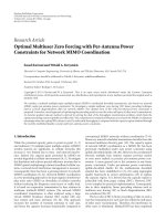
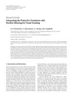
2.1. Camera FOV. TheFOVofacameraisdefinedasa
fan-shaped area as in Figure 1, where CAB defines the FOV
of a camera C. The length of CA or CB is denoted by R,
which defines the distance from the camera to the most
distant objects that appear with an acceptable resolution. The
camera angle of view is denoted by 2α.Thevectord defines
the orientation of the camera and θ is the azimuth. We use
(R, α) to note the type of the camera.
2.2. Camera Viewing Coverage. Under aforementioned cam-
era FOV model, the viewing coverage c ofacamerais
defined as the ratio of the area of the FOV of the camera
to the total monitored area S as c
= αR
2
/S. In the camera
network, the observed regions of different cameras may be
overlapped with each other. We use an approximate approach
to calculate the coverage of a camera network. The total
monitored area is divided into small regular grids. The
coverage is then defined as the ratio of the number of covered
grids to the total numbers of grids:
c
=
number of covered grids
total number of grids
. (1)

2.3. Camera Number versus Network Coverage. Suppose N
cameras of the same type (R, α) are distributed randomly
over an area S.Thecoveragec, defined in the previous
subsection as a probability of the total area being covered, can
be estimated as follows [9]:
c
= 1 −

1 −
αR
2
S

N
(2)
or
N
=
ln
(
1 − c
)
ln
(
S − αR
2
)
− ln S
.
(3)

Our simulations indeed showed that these equations are
satisfied well for real situations. From (2) we can observe
EURASIP Journal on Image and Video Processing 3
α
α
θ
A
B
X
Y
d
R
C(x, y)
Figure 1: The FOV of a camera. The camera is located at C and
oriented at θ.2α is the camera angle of view. The fan area between
CA and CB is the FOV of this camera.
that the expected coverage can be improved by adding more
cameras. However, when N is large enough, adding more
cameras is not effective any more. On the other hand, if we
can adjust the orientation of the cameras to decrease the
overlap of the VOF of the cameras, we can save a lot of
cameras.
2.4. Coverage Optimization Problem. Suppose N cameras of
the same type (R, α) are randomly dist ributed in a two-
dimensional space. Each camera cannot change its location,
but may adjust its orientation to any direction. A control
center receives information about the orientations of all
cameras and can adapt them accordingly (e.g., through the
PTZ mechanism). The object ive of the control center is
then to determine the optimal orientations of all cameras,

(θ
1
, θ
2
, , θ
N
), so that the total coverage of the whole camera
network becomes maximized.
3. PSO for the Coverage Improvement
Our objective is to find the optimal orientation for each
camera. But since the objective function (1) cannot be
differentiated, the traditional g radient descent method will
not work. PSO is a global optimizer which uses random
search and does not require the objective function being
differentiable. Moreover, it has shown good performance in
many engineering optimization fields. Therefore we choose
PSO to optimize the coverage of the camera network.
3.1. Concepts of PSO Algorithm. PSO was proposed by
Kennedy and Eberhart (1995) to model birds flocking and
fish schooling for food [16]. Since then it has been improved
and applied in a lot of science and engineering fields. Similar
to the genetic algorithm, a population of particles is used
to search the solution space of an optimization problem.
Each particle has a position vector and a velocity vector. The
position vector is a potential solution of the optimization
problem, and the velocity vector represents the step length of
the update of the position. During the iterations of the PSO
algorithm, all the par ticles vary their positions and velocities
to search for the best solution. The optimal position found by
the particles swarm is the final solution of the optimization.

The basic framework of PSO for optimizing an objective
function f (x) can be described as follows:
Step 1. Randomly generate m position vectors, x
1
, x
2
, , x
m
,
each one is regarded as a particle and represents a potential
solution of the optimization problem.
Step 2. Randomly generate m velocity vectors, v
1
, v
2
, , v
m
,
where v
i
is the step length for the update of x
i
.
Step 3. Initialize m private best positions, p
1
, p
2
, , p
m
,by

setting p
i
= x
i
,wherep
i
stores the best solution found by
particle i during its history of updates. The evaluation of
a position vector being best or not is based on f (x), the
objective function of the optimization problem.
Step 4. Initialize a global best position g,whereg is the best
among p
1
, p
2
, , p
n
.
Step 5. While the stop criteria are not satisfied,
(1) for i
= 1, 2, , m, update each velocity vector v
i
by
(4)
v
i
:= C
1
× v
i

+ C
2
× rnd
()
×

p
i
− x
i

+ C
3
× rnd
()
×

g − x
i

,
(4)
(2) for i
= 1, 2, , m, update each position vector x
i
by
(5)
x
i
:= x

i
+ v
i
,(5)
(3) for i
= 1, 2, , m, reevaluate each position vector x
i
,
and set p
i
= x
i
if x
i
is better than p
i
,
(4) set g to be the best among p
1
, p
2
, , p
m
.
Step 6. Output g as the final solution of the optimization
problem.
In the above PSO algorithm, searching for the optimum
is an analogy to the particle swarm flying in the space. The
key step is to get the velocity vector by (4), which defines the
step length of the position update during the search. C

1
, C
2
,
and C
3
are constants and rnd() is a random number in (0, 1).
Checking the right part of (4), we can see that v
i
is composed
of three components. The first one means that the flying is
affected by the velocity in the last iteration. Therefore C
1
is
often called the inertia factor. The second part means that
the flying is affected by the private best position memorized
by the particle. And the third part means that the flying is
also affected by the global best position memorized by the
system.
From (4) we can see that if the flying of each particle is
attracted by the best particles found in the swarm, then a
lot of exploitation will be performed near the best particle,
and the convergence of algorithm can be assured. However,
too fast convergence will make the algorithm fall into a local
minimum. PSO uses the inertia factor and the rnd() to make
the particles deviate from directly flying to the temporary
4 EURASIP Journal on Image and Video Processing
(1) Randomly generate mN-dimensional orientation vectors x
1
, x

2
, , x
m
,andmN-dimensional velocity vectors
v
1
, v
2
, , v
m
. Then evaluate the coverage based on these orientation vectors and get the first private best
position p
1
, p
2
, , p
m
and the global best g.
(2) While the predefined iterations is not reached
(3) for each particle i
= 1 to m
(4) calculate v
i
as (4);
(5) calculate x
i
as (5)
(6) transform x
i
in to [0, 2π) and evaluate the coverage based on x

i
(7) if x
i
is better than p
i
, then update p
i
.
(8) if x
i
is better than g, then update g.
(9) end for
(10) end while
(11) output the global best position g, and the obtained coverage.
Algorithm 1: The PSO algorithm for the coverage optimization.
best particle. Then much more space around can be explored
and the algorithm can jump out from a local minimum. This
explains why the PSO generally has a good performance.
3.2. PSO for the Coverage Improvement. The “position vec-
tor” defined in the general PSO is a potential solution x when
we optimize an objective function f (x). The key problems
for applying PSO are to define the position vector x and the
objective function f (x). To avoid confusion, we use for the
cameras the terms “locations” and “orientations” instead of
the “positions” throughout this paper.
In our coverage improvement problem, we need to
optimize the orientation vector of the cameras, x
=
(θ
1

, θ
2
, , θ
N
). The objective function is the total coverage
defined in (1). The computation of (1) is based on the
orientations, locations, and the type parameters (R, α)of
all cameras. The locations and the type parameters of the
cameras are the inputs to the algorithm. The orientations are
what will be searched for. For all the experiments, we follow
[22]tosetC
1
= 0.729 and C
2
= C
3
= 1.49445 in (4).
In standard PSO, the velocity v is often bounded in a
range of (
−V max, Vmax) to a void a long jump of x that may
result x(i) missing the optimum. In our experiments, we do
not limit the velocity, but transform the orientation of the
camera to a value in the range of [0, 2π). Then the update of
the x is also bounded.
The algorithm will stop when the number of iterations
is equal to a predefined number, or a predefined coverage is
reached. Because the locations of the camer as are randomly
generated, we cannot predefine the coverage. Therefore in
practice we often use a predefined maximum number of
iterations. T he complete algorithm is listed in Algorithm 1.

4. Experiments and Results
Three experiments were carried out to demonstrate the
performance of the PSO for the coverage improvement of
cameras. In Experiment 1, the performance and convergence
of PSO were studied. In Experiment 2,PSOandPFCEA
were compared to each other and the advantages of PSO
0.5
0.55
0.6
0.65
0.7
0 100 200 300 400 500 600 700 800 900 1000
Iteration
Coverage
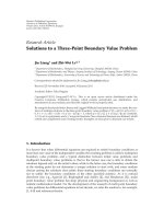
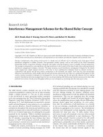
Figure 2: The convergence curve of PSO on a 500 × 500 area with
150 randomly distributed cameras.
Table 1: The statistical data about the coverage improvement.
Algorithm Mean Stdvar
PSO 0.13 0.009
PFCEA 0.07 0.018
were shown by the statistical data. In Experiment 3, the
relationships between the coverage improvement and the
configuration of the camera networks, including the number
of the cameras and the type parameters of the cameras, were
investigated.
Experiment 1. In this experiment, the monitored area was set
to be a 500
× 500 rectangle, and 150 cameras were r andomly
distributed in the rectangle. Each camera was of type (R
=

40, α = π/4). To calculate the coverage, the rectangle was
divided into 500
× 500 unit grids. For the PSO algorithms, 20
particles were used and the max iteration number was set to
1000.
The global best coverage found in the first iteration was
0.52. After 1000 PSO iterations, the coverage was improved
to 0.65. The convergence curve is displayed in Figure 2.The
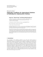
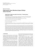
pictures of the initial layout and the final layout of the camera
network are shown in Figure 3.
EURASIP Journal on Image and Video Processing 5
(a) (b)
Figure 3: The coverage improvement of the PSO. (a) the initial layout. (b) The final improved layout.
As indicated by (2), 150 cameras are expected to reach
the coverage of 0.53. Our initial placement with the coverage
of 0.52 was close to this. After the 1000 cycles of PSO,
the coverage was raised to 0.65, that is, the coverage was
improved for about 0.13. If we want to get this coverage
without optimization, we will need to add another 58
randomly placed cameras (total of 208 cameras) as can be
seen in Figure 2.Inotherwords,wehavesaved58cameras
by improving the coverage using the PSO.
Note that the improvement of the coverage varies with
respect to the ra ndom initial configuration of the network,
but in Experiment 2 we will show that the coverage improve-
ment of the PSO is often stable.
Experiment 2. To show the performance of the PSO further,
we ran the program for 30 runs with the same camera num-
ber, camer a type, and PSO parameters as in Experiment 1 .
We collected the coverage improvement data, where each

run started from a random initial configuration. We also
implemented PFCEA as described in [9, 10]tomakea
comparison. In PFCEA, if the virtual torque was greater than
10
−6
, the camera was rotated for π/180, otherwise the camera
was regarded to be in equilibrium. The iteration of PFCEA
was set to 360 in order for each camera to rotate for a full
round (Our experiences also showed that 360 iterations are
enough for the convergence of PFCEA, and more iterations
did not improve the coverage any more.) The collected
statistical data about the coverage improvement is shown
in Table 1. From this we conclude that our PSO statistically
more significantly improved the coverage than PFCEA and
the performance was more stable.
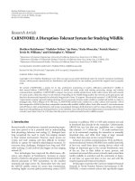
Actually, because of the limitation of the underlying
principle employed, Tao et al.’s PFCEA algorithm cannot
achieve the best possible optimization in a camera net-
work. As illustrated in Figure 4(a), the two cameras are in
equilibrium but the coverage of the two cameras is not as
large as in Figure 4(b). In view of the optimization, PFCEA
tries to use the virtual force as the gradient to search for
A
B
(a)
A
B
(b)
Figure 4: An illustration of the disadvantage of PFCEA algorithm.
(a) Since the two cameras are not allowed translational movement,

they are in a balance state. This configuration is considered as the
optimal solution by PFCEA but it is not really optimal because
of the existence of overlaps. (b) A possible state with maximal
coverage.
the orientations, but because the cameras cannot move, its
optimization ability is always limited.
Experiment 3. In this experiment, the relationships between
the coverage and the three parameters N, R,andα were
investigated, and our PSO algorithm was further compared
with the PFCEA of Tao. In each calculation, the positions of
all the cameras were randomly generated and fed to PSO and
PFCEA identically. The settings for PSO and PFCEA were the
same as in Experiments 1 and 2.
The experiment was carried out in three phases with
marginally varying the 3 parameters. Firstly we varied N,
keeping R,andα fixed. Then we var ied R, keeping N,and
α fixed. Finally we varied α, keeping instead N and R fixed.
The parameters of the camera networks are shown in Tab le 2,
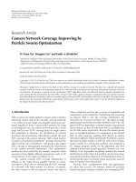
the results are illustrated in Figure 5.
The main results that we can conclude from Figure 5 are
the following.
(a) PSO performed better than PFCEA in all three
phases. In mostcases, the coverage improvement of
6 EURASIP Journal on Image and Video Processing
Table 2: The parameters of the camera networks in Experiment 2.
SN R α
Phase 1 500 × 500 rectangle Varied from 50 to 600 40 π/4
Phase 2 500
× 500 rectangle 100 Varied from 20 to 100 π/4
Phase 3 500

× 500 rectangle 100 40 Varied from π/6 to 3/4π
0
0.2
0.4
0.6
0.8
1
50 100 200 300 400 500 600
Number of cameras
Coverage
Expected coverage
Coverage by PSO
Coverage by PFCEA
(a)
0
0.2
0.4
0.6
0.8
1
Coverage
Expected coverage
Coverage by PSO
Coverage by PFCEA
20 40 60 80 100
R of FOV
(b)
0
0.2
0.4

0.6
0.8
1
Coverage
Expected coverage
Coverage by PSO
Coverage by PFCEA
2/12π 3/12π 4/12π 5/12π 6/12π 7/12π 8/12π 9/12π
α of FOV
(c)
0
0.05
0.1
0.15
0.2
0 0.2 0.4 0.6 0.8 1
Expected coverage
Coverage impr ovement
Number of cameras
α of FOV
R of FOV
(d)
Figure 5: The relationships between the parameters and the coverage. (a) Relationship of (c, N); (b) relationship of (c, R); (c) relationship
of (c, α); (d) relationship of the coverage increment by PSO and the initial coverage.
PSO was nearly twice as large as that of PFCEA.
We believe that this is because PSO is a global
optimization technique and the global coverage is
the objective of this optimization. In contrast, the
objective of PFCEA is balancing the virtual torque
and the optimization of coverage is indirect. There-

fore no global optimal coverage can be obtained.
That is why in some rare cases PFCEA even decreases
the coverage, as can be seen in Figure 5(c) (camera
angleofviewequalto2/12π, the initial coverage
equal to 0.279, and a fter the processing of PFCEA, the
coverage became 0.267).
(b) when the initial coverage was very small or very large,
the improvement was small. This finding was first
claimed in [9], and consistent with the experiments
in this paper, as shown in Figure 5(a), 5(b),and
5(c). The reason to this is that if the initial coverage
is very small, the overlap between the FOV of the
cameras will also be small in general, and then the
improvement cannot be very large. A contradictory
case is that the small initial coverage is caused by
the heavy overlap of FOV, but because the initial
deployment is random, the coverage should obey (2),
then this special case rarely appears. On the other
hand, when the initial coverage is very large, there
is little space left for improvement, and then it is
impossible for any algorithm to find large uncovered
spaces.
(c) to get a clearer picture about the relationship between
the initial coverage and the coverage improvement,
we used the initial coverage as x-axis and the coverage
improvement as y-axis, and we got three curves as
in Figure 5(d), which are derived from Figures 5(a),
5(b),and5(c). We can observe again that, when
EURASIP Journal on Image and Video Processing 7
0

0.2
0.4
0.6
0.8
1
1.2
50 100 150 200 250 300 350 400 450 500 550 600
Number of camera
Expected coverage
Expected coverage
Upbound of coverage
(a)
0
0.05
0.1
0.15
0.2
0.25
0.3
0.35
0.4
0 0.1 0.2 0.3 0.4 0.5 0.6 0.7 0.8 0.9 1
Expected coverage
Coverage improvement
(b)
Figure 6: Relationship of the coverage improvement and the expected coverage. (a) Curves of expected coverage, upper bound of coverage;
(b) relationship of the expected coverage and the coverage improvement.
the initial coverage was too small or too large, the
improvement was small. When the initial coverage
was near 0.6, the PSO obtained the greatest coverage

improvement.
5. Discussions
5.1. The Expected Coverage for the Probably Maximal Cover-
age Improvement. The experiments in the previous section
demonstrated that the PSO can improve the coverage the
most when the initial coverage is about 0.6 but has less effect
when it is close to 0 or 1. Considering that we can get the
expectation (expected coverage) of this initial coverage by
(2), we will explain the results theoretically. That is, we want
to show that when the expected coverage is near 0.6, there
will be maximum space for the improvement.
Assuming that there is no overlap between any two
cameras in a camera network, we have a maximum covered
area. Therefore, we can define the upper bound of the
coverage (c
ub
)ofN camera s in type of (R, α) as follows.
c
ub
= min

NαR
2
S
,1

. (6)
With (2)and(6), we then have an upper bound of the
coverage improvement
delta

−
c
ub
= min

NαR
2
S
,1

−
⎛
⎝
1 −

1 −
αR
2
S

N
⎞
⎠
. (7)
Let us consider the relationship of delta
−
c
ub
and N with
(R, α)andS being constant. From (7) we can conclude that

delta
−
c
ub
is a monotonically increasing function of N when
NαR
2
/S ≤, and a monotonically decreasing function when
NαR
2
/S ≥ 1. Then we get the maximum improvement when
NαR
2
/S = 1.
Replacing αR
2
/S with 1/N in the expected coverage (2),
c
= 1 −

1 −
αR
2
S

N
= 1 −

1 −
1

N

N
. (8)
We know that when N is large enough (e.g., above 100 in
this paper), (1
− (1/N))
N
→ e
−1
yielding c = 1−e
−1
= 0.635.
This means that w hen the expected coverage near 0.6, we
could get the maximum coverage improvement. This value
is close to our observations from the experiments.
In Figure 6(a) we plot the expected coverage c and the
upper bound of the coverage c
ub
as the function of N,where
S is set to 500
× 500, cameras are of type (R = 40, α =
π/4). From this fi gure we derive Figure 6(b) in which we
plot the coverage improvement delta
−
c
ub
as a function of the
expected coverage c.InFigure 6(b), we can clearly see that
the upper bound of coverage improvement is small when the

expected coverage is near 0 or 1, and is maximal when the
expected coverage is near 0.6.
5.2. Adaptive ROI with the Proposed PSO. PFCEA adjusts
the orientations of the cameras to enlarge the FOV of the
camera network. However, the larger FOV does not always
mean higher coverage. Some applications need the camera
network to cover a special region of interest (ROI). As PFCEA
cannot relate the ROI with the FOV of the camera network,
new approaches must be developed. In our proposed PSO,
ROI and FOV are related by (1), so our method can work
well without any modification.
Always, constraints should be considered in real appli-
cations, such as ROI differences, and the occlusions by
obstacles. We still assume that the cameras are already
installed, and we are required to adjust orientations of the
cameras to improve the coverage of the network. Given that
areas that are not in the ROI need not be covered, the
definition of coverage is changed into
c
=
number of covered grids in ROI
total number of gr ids
. (9)
(a) D ifferent ROI at Different Time. In some applications,
the ROI of the system varies depending on the surveillance
objective. For example in Figure 7, two cameras installed on
the wall should monitor A
1
(working area) in the daytime,
8 EURASIP Journal on Image and Video Processing

C
1
C
2
A
1
A
2
A
3
(a)
C
1
C
2
A
1
A
2
A
3
(b)
Figure 7: The results of PSO for different ROIs. (a) Two cameras C
1
and C
2
are arranged to monitor A
1
in the daytime. (b) They monitor
A

2
and A
3
in the night.
C
1
C
2
A
B
(a)
C
1
C
2
A
W
B
(b)
Figure 8: The results of PSO when ROI is occluded. (a) Camera C
1
monitors A and camera C
2
monitors B. (b) When the obstacle W appears,
PSO finds new orientations for the two cameras.
monitor A
2
and A
3
(two doors) in the night. The size of room

is 100
× 100. The area A
1
is a rectangle of 30 × 60 and located
near the center of the western wall. The area A
2
and A
3
are
rectangles of 10
× 20 and located at the two corners beside
the eastern wall. Two cameras C
1
and C
2
are of type (R = 60,
α
= π/2) and installed at the center of northern and southern
wall of the room.
Then we can use PSO to compute the optimal orientation
of the two cameras in the two periods. The results are listed
in Tab le 3, and shown in Figures 8(a) and 8(b) illustrating the
solution in the daytime and the night. Note that because the
ROI in the daytime and in the night is different, we cannot
compare the coverage in the two cases.
(b) ROI Is Occluded by Obstacle(s). In this example shown in
Figure 8, a room of 100
× 100 is monitored by two cameras
C
1

and C
2
,whereC
1
located at the northwest corner and C
2
located at the southeast corner a nd both cameras are of type
Table 3: The orientations of the cameras by PSO for different ROI.
Orientation of
C
1
(radians)
Orientation of
C
2
(radians)
Coverage
Day time
2.330290163 3.732819163 0.2234
Night
0.128384856 5.845456163 0.0410
(R = 100, α = π/4). The ROI is the area occupied by two
rectangles A and B with the same size of 50
× 50.
At first, we get a solution by PSO as in Figure 8(a),where
camera C
1
is arranged to monitor area A and camera C
2
is

arranged to monitor B. Figure 8(b) shows the solution when
an obstacle W appears in the room and the initial FOV of
C
1
is occluded. As a result, the PSO provides a new solution,
letting C
1
monitor B and C
2
monitor A. The results are listed
in Table 4 . We note that the coverage is maintained after the
adjustment of the orientations of the two cameras.
EURASIP Journal on Image and Video Processing 9
Table 4: The orientations of the cameras by PSO for obstacles.
Orientation of
C
1
(radians)
Orientation of
C
2
(radians)
Coverage
No obstacle
0.384704775 3.524939082 0.4475
Obstacle W
1.182262775 4.322527082 0.4475
6. Conclusions
In this paper, we proposed a PSO algorithm to greatly
improve the coverage of a camera network in which the

orientation of each camera can be freely adjusted. Our
results showed that the coverage can be greatly improved
by adjusting the orientation of each individual camera. In
this way we may save a large amount of cameras. T he
algorithm can improve the coverage the most when the initial
coverage is about 0.6. But it has less effect when the initial
coverage is near 0 or 1. Our way of optimizing the camera
network coverage problem outperforms current solutions
from PFCEA. We also showed that our approach can deal
with variable ROIs and with occlusions. Our findings suggest
that the optimization of orientations of cameras should
attract more attentions in the design of camera networks.
We further believe that the method provided in this paper
can be applied in the camera networks to adjust not only the
orientation but also the position of the camera.
Acknowledgments
The authors thank all the anonymous referees for their
helpful comments. This research is suppor ted by the National
Natural Science Foundation of China (60972162), the Sci-
ence Funding of Hubei Provincial Department of Education
(Q20101205), Program of Science and Technology R and D
project of Yichang (A2010-302-10), and the Science Funding
of CTGU (KJ 2009B014).
References
[1] B. Lei and L Q. Xu, “Real-time outdoor video surveil-
lance system with robust foreground detection and state-
transitional object management,” Pattern Recognition Letters,
vol. 15, pp. 1816–1825, 2006.
[2] B. Lei and L Q. Xu, “From pixels to objects and trajectories:
a generic real-time o utdoor video surveillance system,” in

Proceedings of the IEE International Symposium on Imaging
for Crime Detection and Prevent ion ( ICDP ’05), pp. 117–122,
London , UK, June 2005.
[3] E. Dunn and G. Olague, “Pareto optimal camera placement for
automated visual inspection,” in Proceedings of the IEEE/RSJ
International Conference on Intelligent Robots and Systems
(IROS ’05), pp. 3821–3826, 205.
[4] G. Olague and R. Mohr, “Optimal camera placement for
accurate reconstruction,” Pattern Recognition,vol.35,no.4,
pp. 927–944, 2002.
[5] A. O. Ercan, A. E. Gamal, and L. J. Guibas, “Camera network
node selection for target localization in the presence of
occlusions,” in Proceedings of the Distributed Smart Cameras,
October 2006.
[6]A.O.Ercan,A.ElGamal,andL.J.Guibas,“Objecttracking
in the presence of occlusions via a camera network,” in
Proceedings of the 6th International Symposium on Information
Processing in Sensor Networks (IPSN ’07), pp. 509–518, April
2007.
[7] A. T. Murray, K. Kim, J. W. Davis, R. Machiraju, and R. Parent,
“Coverage optimization to support secur i ty monitoring,”
Computers, Environment and Urban Systems,vol.31,no.2,pp.
133–147, 2007.
[8] J. O’Rourke, Art Gallery Theorems and Algorithms,Oxford,
New York, NY, USA, 1987.
[9] U. M. Erdem and S. Sclaroff, “Optimal placement of cameras
in floorplan to satisfy task requirements and cost constraints,”
in Proceedings of the 5th Workshop on Omnidirectional Vision,
Camera Networks and Non Classical Cameras (Omnivis ’04),
Prague, Czech Republic, 2004.

[10] Y. C. Hsieh, Y. C. Lee, P. S. You, and T. C. Chen, “An immune
based two-phase approach for the multiple-type surveillance
camera location problem,” Expert Systems with Applications,
vol. 36, no. 7, pp. 10634–10639, 2009.
[11] Y. Yao, C. H. Chen, B. Abidi, D. Page, A. Koschan, and
M. Abidi, “Can you see me now? Sensor positioning for
automated and persistent surveillance,” IEEE Transactions on
Systems, Man, and Cybernetics—Part B, vol. 40, no. 1, pp. 101–
115, 2010.
[12] J. Zhao and S. C. S. Cheung, “Optimal visual sensor planning,”
in Proceedings of the IEEE International Symposium on Circuits
and Systems (ISCAS ’09), pp. 165–168, May 2009.
[13] D. Tao, H. D. Ma, and L. Liu, “Virtual potential field
based coverage-enhancing algorithm for directional sensor
networks,” Ruan Jian Xue Bao/Journal of Software, vol. 18, no.
5, pp. 1152–1163, 2007.
[14] D. Tao, Research on coverage control and cooperative processing
method for vedio sensor networks, Doctoral dissertation, Beijing
University of Posts and Telecommunications, Beijing, China,
2007.
[15] YI. Zou and K. Chakrabarty, “Sensor deployment and target
localization based on virtual forces,” in Proceedings of the
22nd Annual Joint Conference on the IEEE Computer and
Communications Societies (INFOC OM ’03), pp. 1293–1303,
April 2003.
[16] J. Kennedy and R. Eberhart, “Particle swarm optimization,”
in Proceedings of the IEEE International Conference on Neural
Networks, pp. 1942–1948, December 1995.
[17] B. Brandst
¨

atter and U. Baumgartner, “Particle swarm
optimization—mass-spring system analogon,” IEEE Transac-
tions on Magnetics, vol. 38, no. 2, pp. 997–1000, 2002.
[18] F. van den Bergh and A. P. Engelbrecht, “Training product
unit networks using cooperative particle swarm optimisers,”
in Proceedings of the International Joint Conference on Neural
Networks (IJCNN ’01), vol. 1, pp. 126–131, July 2001.
[19] H. Yoshida, K. Kawata, Y. Fukuyama, S. Takayama, and Y.
Nakanishi, “A Particle swarm optimization for reactive power
and voltage control considering voltage security assessment,”
IEEE Transactions on Power Systems, vol. 15, no. 4, pp. 1232–
1239, 2000.
[20] R. B. Xiao, YI. C. Xu, and M. Amos, “Two hybrid compaction
algorithms for the layout optimization problem,” BioSystems,
vol. 90, no. 2, pp. 560–567, 2007.
10 EURASIP Journal on Image and Video Processing
[21] N. Conci and L. Lizzi, “Camera placement using particle
swarm optimization in visual surveillance applications,” in
Proceedings of the IEEE International Conference on Image
Processing (ICIP ’09), pp. 3485–3499, November 2009.
[22] M. Clerc and J. Kennedy, “The particle system—exploration,
stabilty, and convergence in a multidimensional complex
space,” IEEE Transactions on Evolutionary Computation, vol. 6,
no. 1, pp. 53–58, 2002.