Báo cáo hóa học: " Research Article Parametric Time-Frequency Analysis and Its Applications in Music Classification" pdf

Hindawi Publishing Corporation
EURASIP Journal on Advances in Signal Processing
Volume 2010, Article ID 380349, 9 pages
doi:10.1155/2010/380349
Research Article
Parametr ic Time-Frequency Analysis and Its Applications in
Music Classification
Ying Shen, Xiaoli Li, Ngok-Wah Ma, and Sridhar Krishnan
Department of Electrical and Computer Engineering, Ryerson University, Toronto, ON, Canada M5B 2K3
Correspondence should be addressed to Sridhar Krishnan,
Received 14 February 2010; Revised 15 July 2010; Accepted 15 August 2010
Academic Editor: Yimin Zhang
Copyright © 2010 Ying Shen et al. This is an open access article distributed under the Creative Commons Attribution License,
which permits unrestricted use, distribution, and reproduction in any medium, provided the original work is properly cited.
Analysis of nonstationary signals, such as music signals, is a challenging task. The purpose of this study is to explore an efficient
and powerful technique to analyze and classify music signals in higher frequency range (44.1 kHz). The pursuit methods are
good tools for this purpose, but they aimed at representing the signals rather than classifying them as in Y. Paragakin et al., 2009.
Among the pursuit methods, matching pursuit (MP), an adaptive true nonstationary time-frequency signal analysis tool, is applied
for music classification. First, MP decomposes the sample signals into time-frequency functions or atoms. Atom parameters are
then analyzed and manipulated, and discriminant features are extracted from atom parameters. Besides the parameters obtained
using MP, an additional feature, central energy, is also derived. Linear discriminant analysis and the leave-one-out method are
used to evaluate the classification accuracy rate for different feature sets. The study is one of the very few works that analyze
atoms statistically and extract discriminant features directly from the parameters. From our experiments, it is evident that the MP
algorithm with the Gabor dictionary decomposes nonstationary signals, such as music signals, into atoms in which the parameters
contain strong discriminant information sufficient for accurate and efficient signal classifications.
1. Introduction
Since most of the real-world signals are non-stationary, the
study and analysis of non-stationary signals is receiving
more and more attention in the scientific community.
For signal analysis, time series and frequency spectrum
contain all the information about the underlying processes

of signals. But by themselves, the best representations of
non-stationary processes may not be well presented. Due
to the time-varying behavior, techniques which give joint
time frequency (TF) information are needed to analyze
non-stationary signals. Gabor introduced the concept of
atoms and stated that any signal could be described as a
superimposition of a large number of such atoms [1]. Atoms,
also called basis functions, are signals localized in both time
and frequency domains. This signal analysis method devises
a joint function of time and frequency, that is, a distribution
that will describe the energy density or intensity of a signal
simultaneously in time and frequency [2]. Features extracted
from TF analysis contain the combined time-frequency
dynamics of the given signal, as opposed to features along
either the time or the frequency axis alone, as provided by
conventional techniques [3].
The TF distribution is best suited for non-stationary
signals which need all the three axes of time, frequency,
and energy (or amplitude or magnitude) to represent them
efficiently. TF distributions can be only used for representa-
tion and visualization and not for modeling or analysis of
the signals b ecause these techniques are limited to represent
the signals with possible optimum TF resolution, instead of
efficiently parameterizing them [4].
Another approach of TF analysis is called TF decomposi-
tion. This approach is parametric and more suitable for mod-
eling non-stationary signals. In our work, TF decomposition
is used, signals are decomposed into TF atoms, and atom
parameters are analyzed and manipulated directly to extract
discriminant features for signal classifications.

TF decomposition breaks down a signal into elementary
building blocks, TF atoms, to represent the inner structure
and the processes. It can better reveal the joint TF relation-
ship and can be useful in determining the nature of the
many kinds of non-stationary signals. The success of any TF
2 EURASIP Journal on Advances in Signal Processing
modeling lies in how well it can model the signal on a TF
plane with optimal TF resolution.
Different analysis techniques to decompose signals into
TFatoms(orbasisfunctions)havebeendeveloped.Fourier
analysis and wavelet transform are the most common exam-
ples of such signal analysis models. However, in many cases,
the basis func tions are orthogonal to each other, such as for
the cosines and sines func tion in Fourier and wavelets bases.
Orthogonal basis functions are suitable for data compression
applications, but they exhibit drawbacks for modeling non-
stationary signals in feature extraction application. Based on
Heisenberg’s uncertainty principle, wavelets provides good
time resolution and poor frequency resolution at higher
frequencies, and poor time resolution and good frequency
resolution at lower frequencies. On the other hand, shape-
gain vector quantization is designed to approximate patterns
in functions which occur over a range of different gain
values. Since the size of the codebooks needed to cover
the sphere with a given density increases exponentially with
the dimension of the space, the small number of terms
in the expansions place a sharp limit on the dimension
of the space from which functions can be approximated
with an acceptable degree of accuracy. To expand large
signals, such as digital audio recordings or images, the signals

are first segmented into low-dimensional components, and
these components are then quantized. The expansions can
only represent efficiently those structures that are limited to
a single low-dimensional partition. Structures that extend
across the partitions require many more dictionary functions
for accurate representation. Matching pursuit (MP) with
Gabor dictionary is the suitable method for this requirement.
Atoms in Gabor dictionary can reach the best possible TF
resolution. This is due to the fact that the TF resolution is
limited to the lower bound of the Heisenberg’s uncertainty
principle and it has been proven that only Gabor functions
or atoms (Gaussian) satisfy the lower bound condition [4].
Gabor dictionary is also more flexible and adaptive than
wavelets since there is no restriction on windowing patterns
and the scaling parameter is independent of frequency. Thus,
Gaussian func tions have better time-frequency localization
than wavelet packets. Since the expansions are not con-
strained to orthonormal bases, MP is better adapted to the
time-frequency localization of signal structures and more
efficiently perform non-stationary signal decomposition.
Mallat and Zhang [5] have stated that for a given class of
signals, if we can adapt the dictionary to minimize the storage
for a given approximation precision, we a re guaranteed
to obtain better results by MP than decompositions on
orthonormal bases.
MP with Gabor dictionary has been applied in different
application researches. Jiang et al. [6] proposed joint visual-
audio features for generic video concept classification. Audio
descriptors are used based on MP with the bases, that
is, Gabor functions. These descriptors as a supplementary

means combined with the visual features, effectively improve
the concept classification accuracy rate of a short-term video.
In [7], Chu et al. also proposed MP-based method to classify
the ambient environmental sounds. The proposed MP-based
method utilizes a dictionary from which features of ambient
Non-stationary
signal
Audio
(multimedia)
Best feature set
for classification
Matching pursuit
decomposition
Atoms
Discriminatory
parameters
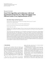
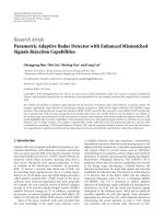
Figure 1: Block diagram of the proposed method for non-
stationary signal classification.
environmental sounds are selected, resulting in successful
classification.
2. Overview of Our Approach
In our work, music signals are being decomposed and
analyzed to classify it into se veral preset categories. A music
signal often includes notes of different durations at the same
time, thus even if a best local cosine basis cannot represent
it well. A music note may have different durations when
played at different times, so a best wavelet packet basis may
not be adaptive and flexible enough to represent this sound.
To approximate music signals efficiently, the decomposition
must have the same flexibility as the composer, who can

freely choose the TF atoms (notes) that are best adapted
to represent a sound [8]. Due to the highly non-stationary
and multicomponent nature of the signals, a more flexible
and adaptive TF decomposition technique, MP with Gabor
dictionary, is utilized to approximate signals and extract the
features for classification. In this work, we propose a para-
metric analysis method to study the atoms obtained from the
decomposition and extract the discriminant features from
the atom parameters.
Figure 1 shows the schematic representation of the
feature extr action, selection, and classification systems used
in our work. Each non-stationary signal is decomposed
into atoms using MP. Atom parameters are analyzed and
manipulated to obtain discriminatory information. Discrim-
inant features are extracted from the parameters. In order
to automatically group signals of same characteristics using
the discriminatory features derived, pattern classification is
carried out using linear discriminant analysis (LDA) tech-
nique. The leave-one-out method is employed to estimate the
correct classification rate with a least bias.
The two experiments cope with music decomposition
and genre classification. From the experiments, it is shown
that the proposed method (see Figure 1) analyzes and
classifies non-stationary signals with acceptable accuracy.
Without any signal segmentations, MP decomposes the
whole non-stationary signal into atoms, and the efficient
classification feature sets are found by analyzing the atom
parameters.
EURASIP Journal on Advances in Signal Processing 3
3. Techniques

3.1. Signal Decomposition Technique:
Matching Pursuit with Gabor Dictionary
3.1.1. Atoms and Dictionary. MP decomposes signals into a
linear expansion of atoms which are well localized both in
time and frequency. Atoms are selected from a predefined
overcomplete dictionary, that is, Gabor dictionary, which
includes functions with a wide range of time-frequency local-
ization and suitable for general decomposition purposes.
The TF base functions (atoms) in Gabor dictionary are
generated by scaling, translating, and modulating a single
Gaussian function g(t). For any scale s>0, frequency
modulation ξ and translation u,wedenoteγ
= (s, u, ξ)and
define
g
γ
(
t
)
=
1
√
s
g

t − u
s

e
iξt

.
(1)
Since a Gaussian function can be transformed into very
different waveforms, the atoms in Gabor dictionary are
very flexible and adaptive, and have good time-frequency
localization. It makes it possible to approximate a non-
stationary signal with an expansion of the atoms selected
from Gabor dic tionary.
Atoms are selected one by one from the dictionary, while
optimizing the signal approximations (in terms of energy) at
each step.
3.1.2. Iterative Algorithm. MP is a greedy signal approxima-
tion algorithm, selecting at least one atom at each iteration
to best match the inner structures of a signal. At the first
iteration, signal f can be decomposed into
f
=

f , g
γ0

g
γ0
+ Rf,(2)
where g
γ0
is the first atom chosen from the dictionary, Rf is
the residual function after approximating f in the direction
of g
γ0

, f , g denotes the inner product of the signal f and
the selected atom g,andg
γ0
is orthogonal to Rf.
In (2), to minimize
Rf, g
γ0
is chosen from the
dictionary so that
|f , g
γ0
 is maximum. In some cases, it is
only possible to find an atom g
γ0
that is almost the best in the
sense that




f , g
γ0




≥
α sup





f , g
γ




,(3)
where α is an optimality factor that satisfies 0 <α
≤ 1[9]. In
the above e quation, sup stands for “supremum”. A value is a
supremum with respect to a set if it is at least as large as any
element of that set.
Thechoiceofg
γ0
is not random. It is defined by a
choice function. The axiom of choice guaranties that there
exists at least one choice function, but in practice, there are
many ways to define it, which depends on the numerical
implementation.
MP is an iterative algorithm that subdecomposes the
residue Rf by projecting it on a base function in the
dictionary that matches Rf almost at best, as it was done
for f .AfterM iteration, the signal f can be decomposed in a
concatenated sum,
f
=
M−1


n=0

R
n
f , g
γn

g
γn
+ R
M
f ,(4)
where g
γn
is the nth base function selected from Gabor
Dictionary, with scale s
n
, translation u
n
and frequency
modulation ξ
n
,andR
M
f is the residual after M iterations.
Thus, signal f can be expressed as a linear expansion
of M base functions selected from the dictionary and the
residue.
3.1.3. Faster Implementation of Matching Pursuit. The main
disadvantage of MP is the high computational complexity

required to repeatedly calculate all the inner products and
search in the overcomplete dictionary for the best atom. In
order to lower the computational cost and accelerate the
signal decomposition process, the iterative process can be
stopped before the residual component will be decomposed
completely, and the search for the atoms that best match the
signal residue can be limited to a subdictionary.
There are two ways to stop the iterative process: one is
to use a prespecified limiting number M of the TF atoms,
and the other is to check the energy of the residue R
M
f .In
this algorithm, the pursuit iterations are preset to M.The
signal decomposition is stopped after extracting the first M
TF atoms. The number of iterations M is selected according
to the size of samples and the complexity of classification. As
long as the atoms extracted contain sufficient discriminant
information to classify the sample into the preset categories,
a smaller number of M is preferred. Therefore, in this work,
the number of iterations is relatively small, and thus the
computational complexity is relatively low.
Instead of searching in a very redundant dictionary, the
search for the atoms that best match the signal residues can
be limited to a subdictionary, w hich can be much smaller
than the original dictionary. This faster version of MP is
implemented as follows: in order to further lower the com-
putational cost and accelerate the decomposition process, the
pursuits are performed only on a set of maximum atoms
which correspond to the most energetic local maxima, that
is, the small areas on the spectrogram of a signal or its

residue with the highest energy concentration (both in time
and frequency). When no qualified atoms are left (either
because they have all been selected or because after a few
iterations their energy is too low), then the corresponding
spectrograms are updated (using the residual), and a new
set of maximum atoms are selected [10]. The algorithm
performs the pursuit on this new set and so on. To use this
faster decomposition, the number of maxima in the set needs
to be specified. If the number is 1, then this method is exactly
equivalent to the regular MP, which is searching the best
match in the whole dictionary. The more maxima put in the
set, the faster the algorithm and the less accurate the signal
approximation will be.
4 EURASIP Journal on Advances in Signal Processing
Considering the size of the samples and the complexity
of classifications, a relatively large maxima is selected in this
algorithm, as long as the parameters obtained are accurate
enough for classification.
In this study, MP signal decomposition is implemented
using the LastWave signal processing software package [10].
Some explanations about the 17 parameters can be found in
the appendix.
3.2. Classification Scheme
3.2.1. Linear Discr iminant Analysis (LDA). In this work,
pattern classification is carried out using the linear dis-
criminant analysis (LDA) technique in SPSS statistics soft-
ware package [11]. To distinguish among the groups, a
set of discriminating features are selected which measure
characteristics in which the groups are expected to differ.
LDA method tries to find one or more linear combinations

of a set of discr iminating features that best separate the
groups of samples. These combinations a re called canonical
discriminant functions and have the form:
f
= x
1
b
1
+ x
2
b
2
+ ···+ x
10
b
10
+ a,(5)
where x
1
···x
10
is the set of features, b
1
···b
10
and a are the
coefficients and constant, respectively, which are estimated
and derived during the LDA procedure [11].
The procedure automatically chooses a first function
that will separate the groups as much as possible. It then

chooses a second function that is both uncorrelated with the
firstfunctionandprovidesasmuchfurtherseparationas
possible. The procedure continues adding functions in this
way until reaching the maximum number of functions.
3.2.2. Leave-One-Out Method. In this study, the classification
accuracy is estimated using the leave-one-out method which
is known to provide a least bias estimate. In the leave-one-
out method, one sample is excluded from the dataset and the
classifier is trained with all the remaining samples. Then the
excluded sample is used as the test data and the classification
accuracy is determined.
This operation is repeated for all samples in the dataset.
The number of correctly classified cases is used to calculate
the classification accuracy rate. Since each sample is excluded
from the training set in turn, the independence between the
test set and the training set is maintained. In a database
with N examples, N experiments are performed. For each
experiment, N
− 1 examples are used for training and
the remaining example is used for testing. The number
of correctly classified subjects is counted to estimate the
classification accuracy rate. The true error is estimated as the
average error rate on test examples:
E
=
1
N
N

i=1

E
i
. (6)
4. Application in Music Classification
4.1. Possible Application. Music genre hierarchies are typi-
cally created manually by human experts and are currently
used to organize and structure music databases. There are
different perceptual criteria that can be used to characterize
a particular music genre. Traditional music genres consist of
classical, rock, jazz, country, blues, reggae, and so on.
Traditionally music databases stored in computers are
organized and retrieved using one or several of the text
indices, just like other textual information. Although manual
indexing and classification have proved to be useful and
widely accepted, finding a computerized method which
allows efficient and automated classification plus easy and
fast retrieval of music database is of increasing importance.
In this study, a content-based music classification scheme
is proposed and tested. The proposed work may have the
following applications: (1) It is possible to perform the
automatic music classifications and annotations. (2) It allows
users to query music by style in spite of the composer. For
example, the user can search for the music with both Bach
and Mozart style composed by other composers. (3) It can
be used in the personalized content-based music retrieval
(CBMR) system based on users’ preference. A CBMR system
can learn users preferred music style by monitoring the users’
retrieval activities and discover the syntactic patterns from
the accessed music [12].
4.2. Previous Works on Music Classification. Content-based

music recognition has been receiving increasing attention in
recent years. Various algorithms have been proposed. These
works c an be primarily separated into two classes: one deals
with score-based music, and the other deals with raw music
data. The latter is more general and has greater significance.
Most of the existing techniques do not take into con-
sideration the non-stationary behavior of the music signals
while deriving the discriminating features. Samples are
examined in either the time or frequency domain where it
is assumed that the signals are wide sense stationary. The
computational complexity for most of the existing works
is relatively high. And the classifications are mostly among
farther-distanced sound groups, such as speech, music, and
noise, or advertisement, football and news. Only a few works
analyze music signals in joint time-frequency domain, using
true non-stationary tools to extract discriminating features,
where the classifications are among different music styles
which is harder than distinguishing music from other sound
recordings, such as, speech or noise.
In [13], Esmaili et a l. proposed a technique using short-
time Fourier transform (STFT) where features are derived
directly from the time-frequency domain, where 143 music
signals, with 5-second duration in each signal, are classified
into six genres, that is, rock, classical, folk, jazz, pop,
and country. Features extracted include entropy, centroid,
centroid ratio, bandwidth, silence ratio, energy ratio, and
location of minimum and maximum energy. LDA is applied
to test the group classification of cases. The accuracy of
classification reaches 92.3% using the leave-one-out method.
The proposal deals with music signals in time-frequency

EURASIP Journal on Advances in Signal Processing 5
domain, and features extracted reflect the non-stationary
properties of music signals. The computational complexity
is relatively low and classification accuracy is relatively hig h
compared to prev ious works. However, since STFT is used
in this technique, music signals are stil l being segmented
and the determination of optimum window size brings up
challenges and uncertainty in pract ice.
In [14], Umapathy et al. also used MP, the same adaptive
TF decomposition algor ithm employed in our work, to
analyze music samples. The music samples were treated
as true non-stationary signals, and no segmentations were
required. As well, no window sizes need to be determined.
An overall correct classification accuracy reached 90%. Some
important observations were also made, such as, the octave
parameter obtained as a result of TF decomposition exhibits
potential discriminatory abilit y to classify audio signals, and
the octave distribution reflects the spect ral similarities for the
same category of sig n als.
Panagakis et al. [15] applied MP for music classification
as well. In this method, the music recording is represented by
its auditory temporal modulations. These auditory temporal
modulations form an overcomplete dictionary of basis sig-
nals for music genres. The music classification is performed
by assigning each test recording to the class where the
dictionary atoms, that are weighted by nonzero coefficients,
belong to. The features were obtained by utilizing dimen-
sionality reduction methods, such as NMF, PCA, random
projection or downsampling, and not by analyzing the atoms
themselves. The classification accuracy is high when the

feature dimension goes up to a certain large number.
Due to space limitations, the other music discrimination
methods with their comparison results which are not
included in this paper can be found in [15–19].
4.3. Music Sample Processing. Since for classification purpose
somewhat general characteristics of signals in a broad sense
is sufficient, the fast implementation of MP is employed.
The number of pursuit iterations is preset to control
decomposition process, and local maxima is used to limit
the searching area. While ensuring that the atoms extracted
from each music sample are sufficient for a satisfactory
classification, we try to use fewer pursuit iterations and larger
local maxima, to reduce the computational complexity and
achieve a better efficiency.
In the foll owing two experiments, only single-channel
recordings in the music samples are used, and sampling rate
is kept as 44.1 kHz. Thus, a 5-second music clip applied in the
first experiment occupies 441,000 bytes and a 10-second clip
applied in the second experiment occupies 882,000 bytes.
4.4. 6-Group Music Classifications
4.4.1. Sample Decomposition. The database is comprised of
96 pieces of music samples, each sample has the duration of
5 seconds. The samples fit into 6 categories as described in
Tab le 1.
Each music sample in the database is decomposed into
atoms with MP. Atoms extracted from one signal are saved
Table 1: 6-group music database.
Group
number
Group name

Number of
samples
Duration of
each sample
1 Christmas Choir 16 5 seconds
2 Country Music 16 5 seconds
3 Greek music 16 5 seconds
4 Jazz Music 16 5 seconds
5 Rock Music 16 5 seconds
6 Scottish Music 16 5 seconds
in a book, which is a variable type for storing the result
of MP decompositions. The number of iterations of the
pursuit is set to be 1,000. Thus the book for each signal
ends up with 1,000 atoms in it, except if the pursuit stops
before because the residue is zero, which has not happened
in the experiment. For each iteration, a set of 100 maxima is
selected to accelerate the decomposition.
4.4.2. Parameter Analysis and Feature Extraction. All of the
17 parameters introduced in Section 3.1.3 are analyzed and
plotted. It is found that some of the parameters do not
carry much distinguishing information and some parameters
are redundant in meaning. For instance, dim is always “1”
because the number of atoms in word is always “1” in the
experiment. Parameters of status, g2Cos2 and chirpId, are
always “0” in the experiment. Phase plots look similar to one
another. Energy in word is the same in value as energy in
atom, and coeff2ofwordisequivalenttocoeff2ofatom,as
there is only one atom in each word. The parameter coeff2of
atom equals to energy in atom in the experiment.
Inordertodetermineeffective classification feature sets,

6 more discriminant parameters are selected and further
analyzed, that is, energy in atom, octave, freqId, innerProdR,
innerProdI, and realGG.
It is observed that octave and energy for the 1,000 atoms
contain good discriminating information for classification.
Octave is just scaling parameter and it is decided by the
adaptive window duration of the Gabor function. The
distribution patterns of octaves for different music groups
look different. Energy distributions for the first 1,000 atoms
are unique for each group. Thus, it is possible to extract good
discriminant information from octave and energy in atom.
Based on the atom energy distributions, one additional
feature “central energy” is derived in order to attain the best
classification feature set. Having taken the energy impact in
each atom along the frequency axis into consideration, we
assume there is one “super” atom at a frequency location
whose energy can replace all the total energy in all the atoms
and still reflects the actually total energy effect along the
frequency axis. This “super” atom energy is defined as central
energy in the study. Thus, central energy is calculated as
the sum of energy in each atom with the frequency weight
divided by the total frequency.
Inordertofindaneffective discriminant feature set to
classify the 96 music samples into one of the six music
groups, that is, Christmas choir, country, Greek music,
6 EURASIP Journal on Advances in Signal Processing
−10 −8 −6 −4 −20 2 4
4
6
6

6
8
Function 1
1
1
Function 2
Canonical discriminant functions
Class
Group centroids
10
−6
−4
−2
0
2
4
6
8
2
2
3
3
4
5
5
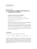
Figure 2: All-group scatter plot with the first two canonical
discriminant functions.
jazz, rock, and Scottish music, supervised classification is
conducted. The parameters of energy, octave, innerProdR,
innerProdI, and realGG, including their derivative values,

for example, the standard deviation of octaves in the first
1,000 atoms, the mean of octaves in the first 1,000 atoms,
the median of octaves in the first 1,000 atoms, and the
derived feature central energy, have been studied and selected
into the discriminant feature sets. The performance of each
feature set is evaluated using LDA. The feature set which
brings up the best classification accuracy will be recognized
as the discriminatory feature for the database.
Observation. (1) In general, combining good features can
bring up better performance. (2) Sometimes, by adding
a good feature to the test feature set, the result is worse
than adding a bad feature. For example, as an individual
feature, the mean of octaves provides better performance
than median of octaves. However, the median of octaves
works better as a component in the test feature set. (3) When
the result reaches a limit, adding more features to the test
feature set does not necessarily bring out better results.
4.4.3. Classifications and Results. After a long try and com-
paring process, the optimum feature set, which brings up
the best classification accuracy, is found to be the standard
deviation of octave, the median of octave, the standard
deviation of innerProdI, the standard deviation of realGG,
and the central energy.
Table 2: Performance of the optimum feature set in LDA classifier
with the leave-out method.
Group
Predicted group membership
Tot al
12 3 4 5 6
Count 1 16 0 0 0 0 0 16

2 0 12 2 0 2 0 16
30 411 0 1 0 16
40 0016 0 0 16
5000016016
6 0 0 0 1 0 15 16
% 1 100.0 .0 .0 .0 .0 .0 100.0
2 .0 75.0 12.5 .0 12.5 .0 100.0
3 .0 25.0 68.8 .0 6.3 .0 100.0
4 .0 .0 .0 100.0 .0 .0 100.0
5 .0 .0 .0 .0 100.0 .0 100.0
6 .0 .0 .0 6.3 .0 93.8 100.0
A scatter plot in Figure 2 is created in SPSS statistics
software package showing the discriminant scores of the
cases on the first two discriminant functions. This plot shows
the separation between different cases. All 96 music samples
are categorized into six groups (Christmas choir, country,
Greek music, jazz, rock, and Scottish music), and the
confusion matrix depicted in Table 2 shows the classification
performance of the optimum feature set. All 16 pieces of
Christmas choir samples, jazz samples, and rock samples are
correctly classified. The other types of music are correctly
classified in a certain rate. For example, 12 out of 16 pieces
of country music samples are well classified, 2 pieces are
misclassified into Greek music group, and the other 2 pieces
are misclassified into rock music group. Using the leave-one-
out method, 89.6% of all original grouped cases are correctly
classified.
4.5. 2-Group Music Classifications
4.5.1. Sample Decomposition. The second database is com-
prised of 112 pieces of music samples with 56 rock-like music

and 56 classical-like music samples, and each sample has
the duration of 10 seconds. All the samples fall into two
categories, that is, rock-like music group (7 subgroups with 8
pieces of 10-second clips in each subgroup), and classical-like
music group (7 subgroups with 8 pieces of 10-second clips
in each subgroup) experiment. The number of iterations of
the pursuit is increased to be 3,000 to get more detailed
information for effective classifications. Thus, the book for
each signal ends up with 3,000 atoms in it, except if the
pursuit stops before because the residue is zero, which has
not happened in the experiment. In order to accelerate the
decomposition, a set of 300 maxima is selected for each
iteration.
We try to use as few atoms as possible to reduce the
computational complexity, as long as satisfying classification
results can be obtained. In this experiment, the first 2,000
atoms are analyzed to find the optimum classification feature
set.
EURASIP Journal on Advances in Signal Processing 7
0 0.5 1 1.5
2
×10
5
Time
0
0.1
0.2
0.3
0.4
0.5

0.6
0.7
0.8
0.9
1
Frequency
Rock-like
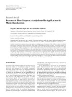
(a) Spectrogram of a rock-like music signal. X-axis: t ime samples. Y-
axis: normalized frequency where maximum frequency corresponds to
sampling frequency/2. Colors indicate different energy levels, with blue
the lowest and red the highest
0 0.5 1 1.5
2
×10
5
0
0.1
0.2
0.3
0.4
0.5
0.6
0.7
0.8
0.9
1
Time
Frequency
Classical-like
(b) Spectrogram of a classical-like music signal. X-axis: time samples. Y-

axis: normalized frequency where maximum frequency corresponds to
sampling frequency/2. Colors indicate different energy levels, with blue
the lowest and red the highest
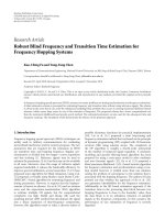
Figure 3: The spectrograms of rock-like music and classical-like music.
In order to l ook more into the characteristics demon-
strated by rock-like music samples and classical-like music
samples, and define the discriminatory features for classifi-
cation, the spectrograms of the samples are also studied. A
spectrogram is the squared modulus of the STFT and is gen-
erally used to display the TF energy distribution over the TF
plane. From the spectrogram plots, it is easy to observe that
in general the energy distribution is different for rock-like
and classical-like music samples. It was found that rock-like
music samples usually contain higher energy components. In
[14], Umapathy et al. studied the MP decomposition algo-
rithm and observed that the octave distribution can reflect
the spectral similarities for the same category of signals. Since
rock-like music samples and classical-like music samples
demonstrate different categorical characteristics with regard
to the spectral energy distribution, it is expected that the
octave parameter may carry distinguishing information to
separate rock-like music samples from classical-like ones.
Spectrograms of one rock-like and one classical-like music
sample are randomly selected from the database and plotted
in Figures 3(a) and 3(b), to show the visible differences of the
spectral energy distribution between the two groups.
4.5.2. Parameter Analysis and Feature Extraction. Knowing
octave may contain important discriminating information
for classification, this parameter, along with its derivative
values such as the standard deviation of octaves in the first

2,000 atoms, the mean of octaves in the first 2,000 atoms,
and the median of octaves in the first 2,000 atoms, has been
studied. The octave and/or its derivatives are selected into the
test feature sets for music g roup classification. The optimum
feature set, which br ings up the best classification accuracy,
is found to be: the standard deviation of octaves in the first
2,000 atoms.
4.5.3. Classification Results and Conclusion. The values of
standard deviation of octaves in the first 2,000 atoms are
listed in Tab le 3. By observation, the threshold of 1.7 is
assigned, which can completely separate the rock-like music
samples from the classical-like music samples. When the
standard deviation of octaves in the first 2,000 atoms is
smaller than 1.7, the music sample is classified into classical-
like music group. When the standard deviation of octaves
in the first 2,000 atoms is larger than 1.7, the music sample
is classified into rock-like music group. The classification
accuracy is 100%.
The experiments on the music databases verify again
that MP, as an adaptive time-frequency tool, decomposes
non-stationary signals into atoms whose parameters contain
good discriminant information for classification. The study
further proves that the octave has the discriminatory ability
to classify audio signals.
5. Conclusion
In this work, MP algorithm with Gabor dictionary is applied
to the decomposition and classification of non-stationary
signals: music signals. It can apply the decomposition on a
signal with any length instead of determining the optimal
window size to segment the signal into pieces. Moreover, by

applying fast approach, the computation complexity can be
reduced, which makes the approach feasible for fast music
classification.
Good discriminating parameters are extracted from atom
parameters obtained from pursuit iterations and analyzed,
and their derivative values, such as mean, median, and
standard deviation, are also calculated and studied. An
additional feature, such as the central energy, is also defined
and derived. The atom parameters and their derivative
8 EURASIP Journal on Advances in Signal Processing
Table 3: Standard deviation of octaves in the first 2,000 atoms of
each music smaple. The four numbers in each row correspond to
the four music samples, respectively.
Music sample
Standard deviation of octaves
Classical 1–4 1.2109 1.1631 1.2701
1.4257
Classical 5–8 1.5357 1.4144 1.0916
1.2308
Classical 9–12 1.0760 1.2239 1.4580
1.1023
Classical 13–16 1.2622 1.1759 1.4090
1.5346
Classical 17–20 1.4979 1.4900 1.4958
1.5222
Classical 21–24 1.4492 1.6053 1.4742
1.3996
Classical 25–28 1.3389 1.2897 1.2771
1.2380
Classical 29–32 1.2351 1.2903 1.3520

1.3613
Classical 33–36 1.3665 1.2858 1.2777
1.1167
Classical 37–40 1.3031 1.4725 1.2384
1.1055
Classical 41–44 1.1702 1.1286 1.1718
1.1266
Classical 45–48 1.3096 1.1946 1.4924
1.1853
Classical 49–52 1.2886 1.1800 1.2341
1.1556
Classical 53–56 1.1894 1.2725 1.3664
1.3428
Rock 1–4 2.1355 2.3155 2.1863
2.0359
Rock 5–8 2.0105 1.9743 2.0570
2.2351
Rock 9–12 2.5278 2.5570 2.3779
2.1647
Rock 13–16 2.2028 2.2540 2.1758
2.0557
Rock 17–20 1.9922 2.0358 2.0630
1.7830
Rock 21–24 2.0853 1.9753 2.0233
1.9941
Rock 25–28 2.0534 1.9518 1.9035
1.9630
Rock 29–32 2.0667 1.8370 1.8492
1.8096
Rock 33–36 2.1048 1.9141 1.8272

1.7141
Rock 37–40 2.0565 2.0237 1.9021
1.7591
Rock 41–44 2.7277 2.5827 2.3621
2.6165
Rock 45–48 2.5539 2.6482 2.6736
2.3581
Rock 49–52 2.4693 2.3978 2.2018
2.1915
Rock 53–56 2.2678 2.1218 2.0843
2.1882
values, along with the additional features, are selected and
combined into various classification features sets. Since
the group labels are preset for all the samples, supervised
classification is conducted. All feature sets are fed to the
linear discriminant analysis classifier (LDA). The classifi-
cation accuracy rate is estimated using the leave-one-out
method. The analysis and classification methodologies are
the same for all two databases. However, since the physical
characteristics are different for each group of signals, the
numbers of pursuit iterations, the values of maxima, and
the optimum discriminating feature sets are different for
different databases, and the classification accuracy rates are
different as well.
It was observed that a combination of good discrim-
inatory features may bring up improved results. It was
also noted that adding more discriminatory features does
not necessary improve the classification performance. The
study proves that the octave has the discriminatory ability
to classify audio signals. It was also discovered that some

other atom parameters besides the octave carry satisfying
discriminatory information as well. The derivative values
of these parameters may act as good discriminant features,
bringing good classification results. The new feature, the
central energy, had a good performance as well. Besides, the
optimum classification feature sets for different databases are
different as well.
In time-frequency (TF) analysis, atoms are usually used
for visualization in TF plane. The study is one of the
very few works that analyze atoms statistically and extracts
discriminant features directly from the parameters. Together
with the similar works done by Umapathy et al. [14]and
Esmaili et al. [13], this work opens a door to the parametric
analysis method in joint time-frequency distribution (TFD).
Appendices
A. Parameters Associated to Word
(i) dim: dimension of word, that is, the number of atoms
contained in each word, for this experiment, it is
always “1”.
(ii) energy in word: always equals to “energy in atom” in
this experiment, as the number of atoms in word is
“1”.
(iii) resEnergy: residual energy in word.
(iv) coeff2 of word: sum of the coeff2ofatoms.Itisalways
equals to “coeff2 of atom” in this experiment, as the
number of atoms in word is “1”.
(v) status: always “0” in this experiment.
B. Parameters Associated to Atom
(i) octave: the scale factor which controls the width of
the window function.

(ii) timeId: related to the discrete time samples where the
atom is localized.
(iii) freqId: related to the center frequency of the atom.
(iv) chirpId: the chirp-rate of the atom. It is always “0” in
this experiment.
(v) innerProdR: the real part of the inner-product
between the signal and the atom.
(vi) innerProdI: the imaginary part of the inner-product
between the signal and the atom.
(vii) phase: used for combining multiple atoms.
(viii) g2Cos2: always “0” in this experiment.
(ix) realGG: the real part of the inner-product between
the complex atom and its conjugate. It is always “0”
for most of the atoms in this experiment.
(x) imagGG: the imaginary part of the inner-product
between the complex atom and its conjugate. It is
always “0” for most of the atoms in this experiment.
(xi) energy in atom: energy in atom. The first extracted
atom contains the largest energy.
(xii) coeff2 of atom: equals to energy in atom in this
experiment.
EURASIP Journal on Advances in Signal Processing 9
Acknowledgment
The authors would like to thank the financial support
received from the Canada Research Chairs’ Program and
the Natural Sciences and Engineering Research Council of
Canada.
References
[1] L. M. Donagh, F. Bimbot, and R. Gribonval, “A granular
approach for the analysis of monophonic audio signals,” in

2003 IEEE International Conference on Accoustics, Speech, and
Signal Processing, pp. 469–472, April 2003.
[2] L. Cohen, “Time-frequency distributions—a review,” Proceed-
ings of the IEEE, vol. 77, no. 7, pp. 941–981, 1989.
[3] S. Krishnan and R. M. Rangayyan, “Automatic de-noising
of knee-joint vibration signals using adaptive time-frequency
representations,” Medical and Biological Engineering and Com-
puting, vol. 38, no. 1, pp. 2–8, 2000.
[4] K. Umapathy, Time-frequency modelling of wideband audio
and speech signals, M.S. thesis, Deparment of Electrical and
Computer Engineeing, Ryerson University, Toronto, Ontario,
Canada, 2002.
[5] S. G. Mallat and Z. Zhang, “Matching pursuits with time-
frequency dictionaries,” IEEE Transactions on Signal Process-
ing, vol. 41, no. 12, pp. 3397–3415, 1993.
[6] W. Jiang, C. Cotton, S F. Chang, D. Ellis, and A. Loui,
“Short-term audio-visual atoms for generic video concept
classification,” in Proceedings of the 17th ACM Multimedia
Conference (ACM MM ’09), pp. 5–14, Beijing, China, 2009.
[7] S. Chu, S. Narayannan, and C C. J. Kuo, “Environmental
sound recongition using mp-based features,” in Proceedings
of the IEEE International Conference on Acoustics, Speech and
Signal Processing, pp. 1–4, 2008.
[8] S. Mallat, A Wavelet Tour of Signal Processing, Academic Press,
San Diego, Calif, USA, 1998.
[9]G.Davis,S.Mallat,andZ.Zhang,“Adaptivetime-frequency
approximation w ith matching pursuits,” Optical Engineering,
vol. 33, no. 7, pp. 2183–2191, 1994.
[10] E. Bacry, “LastWave Documentation,” p
.polytechnique.fr/

∼bacry/LastWave/download doc.html.
[11] SPSS Inc., “SPSS advanced statistics user’s guide,” in User
Manual, SPSS Inc., Chicago, Ill, USA, 1990.
[12] M. Shan, F. Kuo, and M. Chen, “Music style mining and clas-
sification by melody,” in Proceedings of the IEEE International
Conference on Multimedia and Expo, vol. 1, pp. 97–100, 2002.
[13] S. Esmaili, S. Krishnan, and K. Raahemifar, “Content based
audio classification and retrieval using joint time-frequency
analysis,” in Proceedings of the IEEE International Conference
on Acoustics, Speech, and Signal Processing, pp. 665–668, May
2004.
[14] K. Umapathy, S. Krishnan, and S. Jimaa, “Audio signal
classification using time-frequency parameters,” in Proceedings
of the IEEE International Conference on Multimedia and Expo,
vol. 2, pp. 249–252, 2002.
[15] Y. Panagakis, C. Kotropoulos, and G. R. Arce, “Music genre
classification via sparse representations of auditory temporal
modulations,” in Proceedings of the 17th European Signal
Processing Conference (EUSIPCO ’09), August 2009.
[16] S. Lippens, J. P. Martens, T. De Mulder, and G. Tzanetakis, “A
comparison of human and automatic musical genre classifi-
cation,” in Proceedings of the IEEE International Conference on
Acoustics, Speech and Signal Processing (ICASSP ’04), vol. 4, pp.
233–236, 2004.
[17] J. Bergstra, N. Casagrande, D. Erhan, D. Eck, and B. K
´
egl,
“Aggregate features and ADABOOST for music classification,”
Machine Learning, vol. 65, no. 2-3, pp. 473–484, 2006.
[18] D. Ellis, “Classifying music audio with timbral and chroma

features,” in Proceedings of the 8th International Conference on
Music Information Retrieval (ISMIR ’07), pp. 339–340, 2007.
[19] T. Lidy and A. Rauber, “Evaluation of feature extractors and
psycho-acoustic transformations for music genre classifica-
tion,” in Proceedings of the 6th International Conference on
Music Information Retrieval (ISMIR ’05), pp. 34–41, London,
UK, 2005.