Báo cáo hóa học: " Research Article Robust Object Categorization and Segmentation Motivated by Visual Contexts in the Human Visual System" docx

Hindawi Publishing Corporation
EURASIP Journal on Advances in Signal Processing
Volume 2011, Article ID 101428, 22 pages
doi:10.1155/2011/101428
Research Article
Robust Object Categorization and Segmentation Motivated by
Visual Contexts in the Human Visual System
Sungho Kim
Yeungnam University, 214-1 Dae-Dong Gyeongsan-Si, Gyeongsangbuk-Do, 712-749, Republic of Korea
Correspondence should be addressed to Sungho Kim,
Received 7 April 2010; Accepted 9 November 2010
Academic Editor: Steven McLaughlin
Copyright © 2011 Sungho Kim. This is an open access article distributed under the Creative Commons Attribution License, which
permits unrestricted use, distribution, and reproduction in any medium, provided the original work is properly cited.
Categorizing visual elements is fundamentally important for autonomous mobile robots to get intelligence such as novel object
learning and topological place recognition. The main difficulties of visual categorization are two folds: large internal and external
variations caused by surface markings and background clutters, respectively. In this paper, we present a new object categorization
method robust to surface markings and background clutters. Biologically motivated codebook selection method alleviates the
surface marking problem. Introduction of visual context to the codebook approach can handle the background clutter issue. The
visual contexts utilized are part-part context , part-whole context, and object-background context. The additional contribution is
the proposition of a statistical optimization method, termed boosted MCMC, to incorporate the visual context in the codebook
approach. In this framework, three kinds of contexts are incorporated. The object category label and figure-ground information
are estimated to best describe input images. We experimentally validate the effectiveness and feasibility of object categorization in
cluttered environments.
1. Introduction
Intelligent mobile robots should have visual perception
capability akin to that provided by human eyes. Currently,
many researchers have tried to develop human-like visual
perception capabilities such as self-localization and object
recognition for the intelligent mobile robots. Let us imagine
that we have bought a new service robot and put it in our

home environment. The robot should adapt to the strange
environment automatically. It will wander the house and
categorize each room as a kitchen, bath room, or living room.
Additionally, it will categorize novel objects such as the door,
sofa, TV, dining table, chair, or refrigerator. As we can see in
this scenario, the two basic functions of an intelligent mobile
robot are categorizing places and objects for automatic
high-level learning about new environments. In addition,
vision-based categorization system can be helpful for the
visually handicapped people. Such system can give them
useful place and object information. In the current state-
of-the-art, topological localization remains at the level of
image identification or matching to the same environment
[1, 2]. Object identification (recognition) of the same objects
is almost matured due to the robustness of local invariant
features such as SIFT and its generalized version, G-RIF
[3, 4].
Currently, the categorization of general objects or scenes
is an active research area in computer vision society to
realize the helper robots and human assisting vision systems
[5–7]. Therefore, many approaches have been proposed to
handle object categorization. In general, the definition of
object categorization is to assign a category label (normally
basiclevel)foranovelobject.Themaindifficulty of
object categorization is thelarge intraclass variations. Among
many sources of them, such as geometric shape variations
and photometric color variations, textured appearances or
surface markings are dominant in man-made objects as
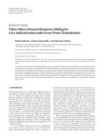
shown in Figure 1. Note the large variations of the surface
markings at the interior regions of the objects. The effect

of surface marking is much larger in man-made objects
than in animals or plants due to creative design for beauty.
These markings degrade the generalization capability of any
categorization methods.
To our best knowledge, there has been few works
published on the reduction of surface markings in object
2 EURASIP Journal on Advances in Signal Processing
Figure 1: Examples of textured objects such as cups, umbrellas, and
ewers (note the different surface markings).
categorization. Until now, most researchers have focused
on how to minimize the intraclass variations caused by
the object shape. We can categorize the current object
representation schemes according to the relation of the
geometric strength and intraclass variation as shown in
Figure 2. As the strength of a geometric relation is weaker,
the handling capability of intraclass variation is higher. At
the same time, the discrimination power is reduced due to
the weak spatial relation. Since the conventional principle
component analysis (PCA) can represent whole objects with
eigen vectors and eigen values, it is relatively weak to handle
the geometric variations [8]. The constellation model of
visual parts can handle geometric variations more flexibly
[5, 9]. It can handle visual variations with the part-based
spring model. Flexible shape samples using geometric blur
can represent large variations of shapes [10]. Bag of words,
derived from document indexing, is a very robust method to
visual variation because it considers no geometrical relations
[11]. Texton, which is a more generalized version of bag of
words, can categorize textured regions such as forest, sky, and
sea [12]. A compromise of both extremes is the implicit shape

model, which assigns pose information for each codebook
[13].
Based on the bag of visual words, extended methods
are proposed, such as spatial pyramid [14], hyperfeatures
[15], and sparse localized features [16] that encode spatial
information to histograms. Zhang et al. focused on classifier
rather than feature extraction [17]. They combine nearest
classifier with SVM, called SVM-KNN that shows upgraded
performance for the Catech-101 DB (66.23%). Varma and
Ray proposed a domain-specific kernel learning method and
obtained a classification rate of 79.85% for the same DB [18].
Perronnin et al. used universal codebooks and class specific
codebooks that enhanced performance but required more
memory space [19]. Wang proposed a discriminative code-
book generation method by introducing multiresolution
codebooks. This obtained superior discrimination compared
to the single-resolution codebooks [20]. Yeh et al. presented
an incremental method for learning a codebook in a dynamic
environment, where images are continuously added to the
database [21]. Gemert et al. introduced uncertainty (kernel
density) modeling in a codebook that suffers less from
the curse of dimensionality [22]. Zhang et al. proposed
a learning method of multiple nonredundant codebooks
for the categorization of complex objects that produced
upgraded categorization performance [23]. However, those
approaches do not consider the exterior variations such as
the background clutter problem explicitly for optimal object
categorization. These methods assume objects as whole
images, so it is very similar to image classification.
If there is background clutter, the above approaches

regard the clutter as parts of objects during learning. If we
learn objects without background clutter and test two sets of
images (segmented, cluttered) using the bag of visual words,
we can obtain meaningful results as shown in Figure 3. These
confusion matrices represent the object categorization for 48
man-made objects of Caltech DB. Note that categorization
accuracy degrades from 90.13% to 60.97% (almost 30%).
Such experimental results are supported by the recent
psychological experiment conducted by Grill-Spector and
Kanwisher [24]. They showed that categorization and figure-
ground segmentation are closely linked.
Several researchers have tried to reduce background
clutter in object categorization. In the feature level, feature
selection [25], or boosting [26] is proposed to overcome
the clutter issue. Leibe et al. proposed combined object
categorization and segmentation with an implicit shape
model (ISM) [13, 27]. First they estimate object category
and then segment the figure-ground pixel-wise. The spatial
relation is modeled in a maximum entropy framework and
leads to a high categorization rate [28]. Direct object region
detection using a boundary fragment, a similar model to
ISM, is also proposed. It shows some promising results
to cluttered objects [29–31]. The partial matching method
such as χ
2
distance can alleviate background clutter during
categorization using SVM [32]. Object segmentation with
given category information using the random field model
shows good segmentation results, even for occluded objects
[33]. Shotton et al. proposed a multiclass object recognition

and segmentation method based on jointly modeling texture,
layout, and context [34]. Recently, Felzenszwalb et al.
proposed an object detection system based on mixtures of
multiscale deformable part model. It can detect deformable
objects on challenging data [35].
All the approaches tried to solve the background clutter
issue in terms of object categorization or object detection
(localizing objects given a category). These methods are par-
tial solutions to our goal, categorization and segmentation
of unknown objects. Now, look at the Figure 4.Doyou
know what it is? This one figure motivates this research work.
HVS can resolve what the object represents: it is a face. In
this paper, our approach is motivated from several biological
findings of human visual systems for the large intraclass
variation and background clutter issues. The next section
summarizes the mechanisms of the human visual system for
visual object categorization in cluttered environments.
EURASIP Journal on Advances in Signal Processing 3
Handling of intraclass variation
Strength of geometric relation
Te x t o n
Bag of
words
Geometric blur
model
Common frame
CM
Constellation
model (CM)
PCA

(global)
Implicit shape
model (ISM)
- Less discriminative
-Robusttovariation
Pose
Pose
Pose
- Discriminative
-Weaktovariation
Figure 2: The trade off between handling capability of visual variation and object discriminability according to the different object
representation schemes: Global PCA-based object representation uses strong pixel relation, which leads to strong discrimination but weak
visual variation. Likewise, texton-based object representation discards pixel relation, which leads to weak discrimination but strong to visual
variation.
Confusion matrix using nearest
neighbor classifier
100
90
80
70
60
50
40
30
20
10
0
45
40
35

30
25
20
15
10
5
Segmented
test image
90.13%
5 1015202530354045
(a) Categorization results for segmented objects
Confusion matrix using nearest
neighbor classifier
100
90
80
70
60
50
40
30
20
10
0
45
40
35
30
25
20

15
10
5
Cluttered
test image
60.97%
5 1015202530354045
(b) Categorization results for cluttered objects
Figure 3: The effect of background clutter to object categorization using the bag of visual words. Confusion matrix measure is used for
comparison.
2. Visual Context in Human Visual System
2.1. Part-Part Context. According to Gestalt’s law, the human
visual system actively utilizes the laws of proximity and
similarity to discriminate the figural region and background
region [36]. Proximity and similarity can group visual
features into the figural region and background region.
Visual context, such as part-part context, can be explained
in terms of such Gestalt law. Part-part context means that
parts belonging to the same object category should have the
same property. Motivated from this psychological finding, we
consider two properties of part relation: the same labeling
and proximity, as shown in Figure 5. Parts belonging to
an object share the same object labels. Furthermore, those
parts are spatially very close. Gestalt’s law of proximity and
similarity for part-part context can provide a group of parts.
Appropriate weights are assigned to those parts according
to the probability of the same labeling and proximity.
Contextually supported parts get stronger weights with a
certain label. Parts belong to background region rarely show
the clustering property compared to parts in the object

region.
2.2. Part-Whole Context. Artale et al.’s research shows that
the part-whole relation has been extensively used to convey
structural information of objects [37]. Part information is
used to predict whole object information (called transitivity
property), such as hands in the human body and nose in
the face. In addition, the interrelations among parts and
whole can help us to recognize objects. Recent neurophys-
iological findings verified that visual recognition processes
are hierarchical and interactively correlated through spike
timing in the ventral visual stream [38]. Therefore, part
information facilitates figure-ground, which also facilitates
object categorization. At the same time, whole category
information facilitates figure-ground segmentation that also
facilitates part detection. Figure 6 represents the simple
4 EURASIP Journal on Advances in Signal Processing
Figure 4: What is this? leaves or stones?
Strong neighbor
support
Weak neighbor
support
ID ID
ID
Same label
Proximity
Figure 5: Similarity and proximity of part-part context.
concept of the part-whole relationship. Visual parts can
predict the figure-ground and object center. Simultaneously,
whole object category information can be used to verify
recognition by carefully analyzing detected parts.

2.3. Ob ject-Place Context. In addition to the part-part
context, and part-whole context, the human visual system
also utilizes object-place context [39]. In general, objects
do not exist in a white background. Instead, objects exist
in certain places, such as cars in a street, hair driers in
a bathroom, and drills in a workshop. Therefore, object
and place (background) are strongly correlated and usually
coexist, as shown in Figure 7. If the relationship between
object and place (background) is stronger, then we can
categorize an unknown object more accurately.
These contexts are modeled by a directed graphical
model that can provide object category with figure-ground
segmentation. Bottom-up evidence from part-part context
and part-whole context can provide the proposal function.
Top-down generative inference using object-background
context and whole-part context can provide the optimal cat-
egory label, region of interest, and figure-ground mask that
can best describe input features (both object and background
features). The inference is conducted by multimodal MCMC
sampling. Experimental results validate the power of the
proposed framework for object categorization and figure-
ground segmentation in a cluttered environment.
Part:
visual parts
Whole:
figure/ground
center
Prediction Verification
Figure 6: Part to whole prediction and whole to part verification in
part-whole context.

Car
Cooperative
Street
Correlated
Object Place
Figure 7: Strong correlation between object and background
(place) context.
3. Biologically Motivated Object Categorization
3.1. Categorization Model of HVS. Conventionally, vision
is considered to be accomplished by a feedforward chain
of computations [40, 41]. Serre et al. also introduce a
hierarchical feedforward system that closely follows the orga-
nization of visual cortex and builds an increasingly complex
and invariant feature representation by alternating between
a template matching and a maximum pooling operation
for object recognition [42]. Pinto et al. found that V1-
like model can recognize objects well [43]. However, recent
neurophysiological experiments have provided a variety of
evidence suggesting that feedback from higher-order areas
(IT) can modulate the processing of the early visual cortex
(V1, V2, V4) [38, 44–46]. A popular theory in the biological
community to account for feedback is based on attention
modulation and biased competition. From that perspective,
visual processing is still primarily a series of feedforward
computations, except that the computation and information
flow are regulated by selective attention. Based on those
neuropsychological findings, we can make a feasible object
categorization model in the ventral visual pathway as shown
in Figure 8. Along the ventral pathway, the specific visual
properties and features to which cells are selective become

more and more complex. See the left image in Figure 8.
The first feature dimension extracted by the visual system
in the retina and present in the LGN is luminance contrast.
In the primary visual cortex, neurons use this input to
build selectivity for line or edge orientation and sometimes
display a certain degree of invariance to complex cells.
Further down the line neurons respond to figure-ground
boundaries in V2, and to complex geometric patterns in
V4. Selectivity for the identity and category of complex
objects or their components arises in the posterior part
EURASIP Journal on Advances in Signal Processing 5
of the inferotemporal cortex (PIT) and is refined as visual
information advances to the anterior part (AIT). Typically,
neurons in IT respond to meaningful objects, in particular
those with obvious biological relevance such as faces. IT
is thus often considered as the end-point of the ventral
stream hierarchy. This hierarchy is widely taken as evidence
for a functional architecture in which, in a sequence of
relatively small computational steps, visual areas extract from
their afferents increasingly complex features of the stimulus
theory. At the last levels, such features are by construction
complex enough to represent object identity or category [38].
Note also that the visual processing modules such as, V1, V2,
V4 are interrelated. Furthermore, each module has bottom-
up analysis and top-down synthesis for the correct image
understanding.
The right image in Figure 8 is the corresponding visual
processes implemented in this paper. Given an image, Gabor
90
◦

phase and Gabor 0
◦
phase images are obtained for
corner and blob center detection. Simultaneously, edge map
is detected for the object boundary points. These processes
are performed in scale space pyramid. Such low level
processing modules are similar to the V1 in HVS. Next,
figure-ground segregation process exists like V2 in HVS.
Dense local invariant structures extracted in V4, then final
object categorization is performed on the top position. Those
functional blocks interact with each other through bottom-
up analysis and top-down synthesis. Details will be explained
in the following sections.
3.2. Object and Category Representation. To fully utilize the
visual contexts, we propose a composite representation of
object instance with region of interest (ROI, object center +
scale), object boundary, and local parts, as shown in Figure 9.
ROI represents the object center with the scale in this work.
An object boundary or figure-ground mask divides an image
into figural region and background region. Finally, local
parts (clustered from dense features) represent the part-
based object appearance. The ROI, figure-ground, and local
parts are interrelated, like the spring model. In this joint
model, local parts have an important role, since they relate
ROI and the figure-ground boundary. That is, if we know a
visual part, then we can predict ROI and object boundary.
This is the part-whole context explained in the previous
section. Every object instance is represented by ROI, Figure-
ground mask, and codebook (including part appearance and
pose).

We represent a category by extending the basic object
representation model, as shown in Figure 10. There are uni-
versal appearance codebook and category-specific appear-
ance codebook in the category representation. Local appear-
ances of visual parts in the object instance are linked to
category-specific codebook (CCB). Part pose information is
stored in each part relative to the object center in the object
instance. Category-specific codebooks are also linked to the
universal codebook (UCB) by comparing visual appearance.
In Figure 10, wheels in the car codebook and in airplane
codebook have a similar appearance. At the same time,
each category also has a contextually related background
codebook. Therefore, each category has a category-specific
codebook and category-related background codebook. In
addition, each UCB contains all possible link information
to CCB. This link information is useful for bottom-up
inference. Details of modeling and learning will be explained
int the next sections.
3.3. Mathematical Formulation for Object Categorization.
Look at the object in a cluttered environment, as shown in
Figure 7. We can generate such images if we have the category
label, ROI (object center + scale), figure-ground mask,
and codebook corresponding to input features belonging to
the object category and category-related background. Fig-
ure 11(a) shows such an example of the generative procedure.
We assume a single object in a cluttered background, since
it is the basic block for multiple object categorization. The
parameter
{C, B} represents a pair of category label C and
related background label B.Givena

{C, B},firstwecangen-
erate the region of interest (ROI) of an object. ROI includes
both object center and relative object scale. Therefore, the
ROI parameter V contains object center (x
c
, y
c
)andobject
scale factor (s) relative to model size. In the next layer, figure-
ground mask (M) is generated using the information of both
category-background label and ROI. Mask M is an array
of
{0, 1}, where 0 represents the background pixel and 1
represents the foreground pixel. In the third layer, codebook
index F is selected using category-background information
and figure-ground mask. The codebook index denotes label
of category-specific codebook as shown in Figure 10.If
the index belongs to the object region, our algorithm will
search it from CCB and if it belongs to the background
region, our algorithm will search it from the background
codebook related to the CCB. Finally, we can generate input
features G using the selected codebook and ROI information.
G consists of a set of local appearance A and part pose
X (total N features). ROI information is reflected to part
pose generation. Figure 11(b) shows the directed graphical
model (Bayesian Net) exactly corresponding to Figure 11(a).
White nodes represent hidden variables and shaded nodes
represent observed variables. Note the causal relationship
between nodes. Due to the N input features, we replicate the
codebook index and observation nodes N times, as boxed

regions. In addition to the top-down generative model, we
draw bottom-up (dotted arrow) flow for fast estimation. This
will be explained in the learning section.
Now, let us formulate the object categorization in clut-
tered images based on the directed graphical model. Given
an unknown object with cluttered background, we can detect
multiscale input features G
={g
i
= (a
i
, x
i
)}, i = 1,2, , N.
a
i
denotes descriptor vector of local patch and x
i
denotes
part position. Assume that we already have trained model
D, which has labels, figure/ground masks, and ROIs with
learned parameters (learning will be explained in the next
section). Then, the object categorization and segmentation
problem is to estimate the category label, C, figure-ground
mask, M(i, j)
= 1or0,andROI,V ={x
c
, y
c
, s}.Weset

the solution vector as H
= (C, M, V) and the solution space
as Ω. Then the optimal solution can be represented by (1).
6 EURASIP Journal on Advances in Signal Processing
Bottom-up analysis
Top-down synthesis
Scale space
pyramid
V1
V2
V4
IT
Gabor 90
◦
phase
(for corner detection)
Gabor 0
◦
phase
(for blob center detection
Edge map for object
boundary points
Figure/ground
Local invariant
features
Distributed category prototypes
(joint appearance and shape model)
Figure 8: The overall flow of object categorization of human visual system.
For 2D object: region of interest
(object center, scale)

Boundary shape
Figure/ground information
Region of interest Figure/ground mask Local appearance
Appearance codebook
part pose
Figure 9: Basic representation of an object instance by region of interest (ROI), figure-ground mask, and local appearance.
Normalization is omitted for the simplicity, as we should
maximize the posterior
H
∗
= arg max
H∈Ω
p
(
H | G, D
)
= arg max
H∈Ω
p
(
H | H,D
)
p
(
H | D
)
.
(1)
According to the directed graphical model (see Fig-
ure 11(b)), the prior term p(H

| D) is decomposed into
three conditional probabilites, as (2). If you want to know
the basics of the graphical model, we recommend you see
[47]. From trained data D, p(C
| D) represents the prior
EURASIP Journal on Advances in Signal Processing 7
UCB: universal codebook
for bottom-up inference
CCB: category specific codebook for
top-down inference
Contextually-related background codebook
Object instance representation: ROI + figure/ground + part
Car Airplane
··· ··· ···
··· ···
···
Figure 10: Category representation by two-layered codebook (universal codebook + category-specific codebook) with object instance
representation.
To p - d o w n
Bottom-up
Codebook index
Figure-ground
ROI
{C, B}
G
F
M
V
N
b1

f2
f1
f3
b3
f5
f4
b2
b4
b5
b6
(a) Example of generative process
To p - d o w n
Bottom-up
{C, B}
AX
F
M
V
N
(b) Corresponding graphical model
Figure 11: (a) Generative framework for simultaneous object categorization and figure-ground segmentation in cluttered environment, (b)
corresponding representation by directed graphical model (Bayesian Net).
of the category label. Given category label C and D, p(V |
C, D) represents the prior of ROI. Given a category, ROI
with trained data, we can generate the figure-ground mask
M from p(M
| C, V, D)
p
(
H

| D
)
= p
(
C | D
)
p
(
V | C, D
)
p
(
M | C,V,D
)
.
(2)
Given a hypothesis H
= (C, V, M) and trained data D,
the likelihood term p(G
| H, D)isfactorizedas(3)
p
(
G
| H, D
)
= p
f

G
f

| H, D

p
b
(
G
b
| H, D
)
,(3)
where G
f
={g
m
: M(x
m
) = 1} and G
b
={g
n
: M(x
n
) =
0}. G
f
denotes the figural feature set and G
b
denotes the
background feature set. In addition, x
m

is the position of
8 EURASIP Journal on Advances in Signal Processing
Figure 12: Foreground objects and detected local features.
Repeatable part
Surface marking part
Surface marking
reduction by
intermediate blurring
Cup instances
Figure 13: Large intraclass variations due to surface markings and
reduction strategy during codebook selection.
the input feature g
m
in the image space. If we assume N
independent input features, each likelihood term is defined
as (4)
p
f

G
f
| H, D

=
N
f

i=1
⎛
⎜

⎝
|
F
f
|

j=1
φ
j
N

a
i
; μ
j
a
, Λ
j
a

·
N

x
i
; s ·μ
j
x
+


x
c
, y
c

, Λ
j
x

⎞
⎟
⎠
,
p
b
(
G
b
| H, D
)
=
N
b

i=1
⎛
⎝
|F
b
|


j=1
φ
j
N

a
i
; μ
j
a
, Λ
j
a

A
⎞
⎠
,
(4)
where N
f
is the number of input features generated by
the object codebook F
f
and N
b
is the number of input
features generated by the background codebook F
b

.Thus,
N
f
+ N
b
= N, the total number of input features. φ
j
is the probability of codebook j. Foreground features are
generated by Gaussian distributions N where μ
j
a
and Λ
j
a
denote mean and covariance of appearance codebook a
i
,
respectively. μ
j
x
denotes the average position of part j.
Note that the codebook mean is affected by the ROI,
V
= (x
c
, y
c
, s). Background features are generated by the
background codebook. However, the pose distribution is
uniform, since they are distributed randomly in area A.

Details of learning and inference will be explained in the next
sections.
4. Learning Parameters
As shown in Figure 10, the category representation scheme
consists of universal codebook and category-specific code-
book. The category-specific codebook should be linked to
the universal codebook. Each codeword is also linked to
all similar parts in object instances. The learning items are
first category-specific codebook, universal codebook, links
between CCB and UCB; second, links between CCB and
local patches in object instances that have ROI, figure/ground
mask, and local patches. Note that training object instances
are reused to handle large intraclass variations. The link
information is a useful cue during bottom-up inference.
From a scene feature, we can find similar UCB. Then, if
we use the link information in the UCB, we can select
the category-specific codebook. The links between CCB and
local patches can give probable ROI, because each part has
object center information. Finally, we introduce how to learn
prior parameters, as shown in (2).
4.1. Step 1: Local Feature Extraction. First, we extract dense
(or sparse) features, called G-RIF (Generalized Robust
Invariant Feature), in scale-space from foreground object
regions, as shown in Figure 12 [4]. G-RIF is similar to the
well-known SIFT, but it is a generalized version of SIFT. It
can detect corner-like interest points from a convolved image
with 90
◦
phase of the Gabor kernel. It can also detect blob
center points from a convolved image with 0

◦
phase of the
Gabor kernel. In addition, we also use randomly sampled
canny edge points, since this can enhance categorization
capability in the codebook approach [48]. After interest point
detection, the scale of local interest point is determined
using the SIFT method. Then, the localized histogram of
edge strength, orientation, hue makes a descriptor in G-
RIF. Positions (x, y) of local features are defined in polar
coordinates based on the object center to reflect object size
changes.
EURASIP Journal on Advances in Signal Processing 9
42
44
46
48
50
52
54
56
Classification rate
01234567
Blur level (σ)
Figure 14: Evaluation of blurring level in terms of categorization rate.
0
1
2
3
4
5

6
7
8
9
H(C
i
| F)
0 50 100 150 200 250 300 350
Low entropy
High entropy
Figure 15: Observation for repeatable parts (high entropy) and surface marking parts (low entropy).
4.2. Step 2: Learning Index of CCB Guided by Entropy.
We have to learn parameters related to codebook for the
likelihood estimation in (4).Acodewordinacodebook
has four components: codeword index (F), probability of
codeword frequency (φ), appearance parameters (mean,
variance for both object and category), and pose parameters
(mean, variance for only the object). The codebook selection
method is important to achieve successful categorization. We
focus on reducing surface markings during visual words or
codebook generation, as shown in Figure 13.Ourstrategies
10 EURASIP Journal on Advances in Signal Processing
0
0.5
1
1.5
2
2.5
3
3.5

4
Entropy (H(L | F))
0 100 200 300 400 500
High entropy
Low entropy
Index of codebook candidate
Category specific codebook versus entropy
Figure 16: Entropy of candidate codebook and corresponding visual features.
0
0.2
0.4
0.6
0.8
1
3
2
1
Low entropy (H(χ
| F), H(σ |F))−→ good codebook
123456
Prob. of scale
p(χ
| F)
p(σ
| F)
Prob. of feature position
0
0.2
0.4
0.6

0.8
1
123456789
(a)
0
0.1
0.2
0.3
0.4
0.5
3
2
1
High entropy
−→ bad codebook
123456
Prob. of feature position
Prob. of scale
0
0.1
0.2
0.3
0.4
0.5
0.6
0.7
123456789
(b)
Figure 17: Probability distribution of a codeword pose (position and scale) and its corresponding parts. We select the final codebook whose
pose entropy is low.

EURASIP Journal on Advances in Signal Processing 11
Figure/ground mask
Codeword F
i
Codeword F
j
θ
r
(r, θ)
χ, σ
Figure 18: Learning CCB pose including figure-ground mask.
Figure 19: Examples of learned codebook overlaid on exemplars. Differentcolorrepresentsdifferent codebook.
are twofold. First, apply intermediate blurring to extract
important object shape information. This is motivated
from the cognitive experiments showing that human visual
systems can categorize blurry objects very quickly and
accuracy performance is virtually unaffected by up to 50%
blurring, but then rapidly falls to a low level, following a
sharp sigmoid curve [39, 49]. This means that low spatial
frequency information is important to visual categorization.
The second is based on the information theory for the code-
book selection. The simplest codebook generation method
is k-means clustering. However, the proposed entropy-
guided codebook can represent repeatable or semantically
meaningful parts removing surface markings.
In advance, we evaluate the effect of blurring by changing
the smoothing level (the standard deviation, σ in Gaussian
blur). G-RIF features are extracted from the blurred images.
Figure 14 shows the evaluation results with the correspond-
ing blurred objects. We use bag-of-keyword method with its

nearest neighbor classifier [11]. According to the maximum
value, we set the blurring level as σ
= 3.
12 EURASIP Journal on Advances in Signal Processing
CCB: Car
CCB: Category
specific codebook
CCB: Airplane
UCB: Universal
codebook
···
··· ···
Figure 20: Learning universal codebook from category-specific codebooks.
1. Input
2. Dense feature
3.Matching to UCB
4. Grouping (similarity
and proximity)
5. Part-part context
(estimate weight)
6. Part-whole context
Category model DB
Car
CCB
···
Background CB
UCB
Final result
Car
10. Check hypothesis

9. Multi-modal
figure-ground mask
8. Multi-modal ROI
7. Car category
Top-down inferenceBottom-up proposals
Airplane
Figure 21: The overall inference flow by boosted MCMC method for simultaneous object categorization and figure-ground segmentation.
Assume that we have finite (ex. 15) images. Through
agglomerative clustering (bottom-up) and k-means cluster-
ing (top-down), we can obtain candidate codebook F
hyp
.
For each codebook candidate F,wecanestimateentropyof
instance label L,as(5)
H
(
L
| F
)
=−

l∈L
p
(
l | F
)
log
2
p
(

l | F
)
,
(5)
where p(l
| F) is the relative frequency of codebook F in
object instance l.
We have to minimize intraclass variations. As mentioned,
one of the main causes of large intraclass variation is
surface markings, which have various texture patterns for
object instances. Figure 15 represents the relation between
entropy of codebook within category and feature positions
in category instances for a cup category. Row axis is the
ID of codebook and column axis is the entropy value of
each codebook within category. As indicated by the arrows,
high entropy codebooks are strongly related to semantic,
parts and low entropy codebooks are strongly related to
EURASIP Journal on Advances in Signal Processing 13
+
e
k
N(k)
Neighboring
evidences
Current interesting
evidence
Figure 22: Concept of part-part context. The quality of current
interesting evidence is determined by neighboring evidences.
surface markings. So, the surface markings can be removed
by finding repeatable parts or high-entropy parts. Figure 16

shows the entropy of the candidate codebook for additional
car category. A codeword whose entropy is low belongs
to nonrepeatable parts, such as surface markings (see the
detected parts in FEDEX) or distinctive parts. A codeword,
whose entropy is high, belongs to repeatable (or semantically
meaningful) parts, such as the wheel parts.
The candidate codebook is first filtered by entropy values
because we also have to consider the statistical property
of pose for each codeword. During initial filtering, we
select codebook candidates whose entropies are larger than
the entropy threshold (0.5, empirically tuned). Based on
such a candidate codebook, we check the pose entropy of
each codeword. In our object instance representation, the
appearance codebook is important to predict the ROI and
figure-ground mask. The more stable the part position, the
more accurate the estimation obtained. If we quantize part
position in the image space and part scale in the scale-space,
as shown in Figure 17, we can estimate the probability of
part position p(χ
| F)forcodebookF. Likewise, we can
estimate the probability of part scale p(σ
| F). Positional
entropy and scale entropy are calculated from this proba-
bility. Figure 17(a) shows a codeword whose pose entropy
(uncertainty) is low and Figure 17(b) shows a codeword
whose pose entropy is high. The final codebook is selected by
thresholding the pose entropy. We choose the final codebook
whose position entropy and scale entropy are less than 1.5
(empirically tuned). The pose entropy is very meaningful
to model object categories. If the pose entropy is high for

all codebooks, then our joint appearance-shape model is
unsuitable, since objects usually have textured (repeated
pattern) surfaces. In such a case, the conventional bag of
keypoint-based category representation is more suitable,
because it discards the spatial distribution of features [11].
4.3. Step 3: Learning Appearance and Pose of CCB. We c an
obtain a category-specific codebook, including codebook
index parameter, through the entropy-guided codebook
selection (using appearance entropy and pose entropy). At
this state, a finally selected codeword has a set of training
features belonging to this codeword. The codebook param-
eters for appearance are estimated by sample mean (μ
a
)
and sample variance (Λ
a
). For simplicity, we consider only
diagonal variance. The parameter estimation of codebook
pose is rather difficult, since instances of a codeword can
be positioned on different locations in a large image. A
Gaussian mixture model can represent such a phenomenon
but the complexity of learning increases. We model the
codeword pose by compromising a nonparametric and
parametric representation scheme, as shown in Figure 18.
The sample mean and sample variance of a codeword pose
is estimated in polar coordinates from clustered features for
each object instance (see the enlarged image). The sample
mean is μ
x
= (χ, σ) = ((r, θ), σ). r denotes the average

distance between the considered part and object center of
the figure/ground mask. θ denotes the relative angle of
considered part reference on the image row-axis.
σ denotes
the estimated standard deviation of pose distribution. This
process is repeated for other object instances to which
the codeword belongs. We assume a uniform distribution
of object instances. Pose information of each codeword
is distributed among object instances through such pose
estimation process. Figure 19 represents a partial examples
of codebook for each instance. Every third codebook is
overlaid to discern a different codebook. Colors in the figure
represent the ID of codewords. Note that similar parts have
the same colors. The parameter estimation (μ
a
, Λ
a
) for the
background codebook is almost the same as the foreground
codebook, except for the codebook pose. We assume that the
pose of the background codebook is randomly distributed in
the image space and scale-space.
4.4. Step 4: Learning UCB from CCB. Up until now, we have
learned the CCB index, appearance, and pose parameters
for each object category. The last learning component is the
universal codebook (UCB) index and appearance parameter
for bottom-up inference. The learning process is quite
simple. As shown in Figure 20, initially we have a set of CCBs,
such as a car, or an airplane. The appearance parameter of
UCB is estimated by agglomerative clustering used in CCB.

Appearance similarity is a useful measure to cluster similar
category-specific codewords. In Figure 20,afrontwheel
of a car category and a wheel of an airplane have similar
appearance. Therefore, appearance of two category-specific
codewords merges into a universal codeword. Following this
process, each universal codeword has the link information
between itself and indices of category-specific codewords.
The link information is useful during bottom-up inference,
as explained in the next section.
4.5. Prior for Category, ROI, and Mask. Prior distributions
in (2) are learned using a set of labeled training images.
Let trained database D have category label C
DB
,ROIV
DB
,
and figure-ground mask M
DB
for each instance. At this state,
parameters related to codebook (φ, μ, Λ) are null. If there
are N
C
categories and each category has N
M
examples, then
the category prior p(C
| D) is uniform as 1/N
C
.Givena
category, the viewpoint distribution can be estimated directly

from labeled examples. However, we define p(V
| C, D),
as p(x
c
, y
c
, s | C, D) = 1/A · 1/1.5 for the generalization.
14 EURASIP Journal on Advances in Signal Processing
With neighbor support Without neighbor support
V
M
(a) The effect of part-part context
Dense sampling
(random + edge: 500
∼)
Sparse sampling
(DoG + Harris: about 100)
(b) The effect of feature point sampling
Figure 23: Properties of online boosting methods: (top row) estimated ROI (object center) points, (bottom row) accumulated figure/ground
masks.
A represents the area of search region. In a real environment,
objects can be anywhere in an image. We restrict the scale
factor in the range of [0.5 2]. Given category label, viewpoint,
and figure-ground masks in D, the prior p(M
| C, V, D)
is defined as 1/N
M
, since we randomly choose the figure-
ground mask in the database.
5. Statistical Inference by Boosted MCMC

We can obtain optimal object categorization and figure-
ground segmentation by solving (1). However, due to the
high dimensionality, direct inference is intractable. We utilize
the approximate inference method using a sampling method,
such as Markov Chain Monte Carlo (MCMC) [50]. MCMC
samples guarantee convergence to the posterior distribution.
The Metropolis-Hastings (M-H) algorithm is often used
for MCMC inference. The original MCMC can provide a
globally optimal solution with the cost of a long time (many
samples). We utilize M-H sampling but we modify the pro-
posal function (q(H
→ H

)) by multimodal distribution. It
consists of prior distribution and boosted distribution from
bottom-up inference (see the dotted arrows in Figure 11(b)).
Samples from multimodal distribution are accepted with
probability α,definedas(6). Figure 21 shows the overall
inference flow graphically. Details of the bottom-up proposal
and multimodal sampling-based inference are explained in
the following subsections.
α
= min

1,
p
(
H

| G, D

)
p
(
H | G, D
)
·
q
(
H

→ H | G, D
)
q
(
H → H

| G, D
)

. (6)
5.1. Bottom-Up Proposal by Context-Based Boosting
5.1.1. Dense Feature Grouping Using Similarity and Proximity.
First, we extract local features at dense points, such as corner,
blob center, and edge samples as shown in Figure 21 ((2)
Densefeature).Theaveragenumberoffeaturesper320
×240
image is 1000. It is inefficient to directly use such a huge
number of features for bottom-up inference. Instead, we
filter out the dense features using discrimination by the k-
NN (nearest neighbor, in this paper k

= 1) classifier with
UCB ((3) Matching to UCB). Then filtered dense features are
grouped according to Gestalt’s law of appearance similarity
and proximity ((4) Grouping: similarity and proximity).
Similar features within 25 pixels are grouped. We denote the
finally grouped features as e. In Figure 21, the image denoted
as (4) Grouping shows the clustered features with the color
index of UCB.
5.1.2. Online Boost Using Visual Context. Given evidence
(e, clustered from dense features), we can directly estimate
the proposal function bottom-up using two kinds of visual
context. The first context is part-whole relation, which is
asortofhierarchicalcontext.Evidence,e
k
, can predict a
codeword in UCB. Since UCB contains CCB links, we can
predict category (C), ROI (V), and figure-ground mask
(M). Figures 20 and 18 will help you understand the part-
whole prediction mechanism. The second context is the part-
part relation. As shown in Figure 22, the quality of current
interesting evidence, e
k
,isaffected by neighboring evidences
N(k). We can predict ROI of e
k
using the part-whole context.
Neighboring evidences can also provide ROI (object center,
relative scale). If these ROIs are compatible to the ROI by
e
k

, then we accept the prediction of the current evidence.
Based on the concept of visual contexts, we can model this
phenomenon mathematically by borrowing the concept of
boosting [51]. In the original boosting, a strong classifier (g)
is constructed from a set of weak classifiers (h
k
), as g(x) =

k
max
k=1
α
k
h
k
(x). The weak classifier weight α
k
is learned off line
using a positive and negative training set.
The joint category and ROI classifier g(C, V, M
| e)is
defined in (7). Given an input evidence e
k
, we can predict
category (C), ROI (V), and figure-ground mask (M) using
the part-whole context, such as evidence to UCB, UCB to
EURASIP Journal on Advances in Signal Processing 15
Figure 24: Robustness for scale changed test set: (first column) estimated ROI points, and (second column) accumulated figure/ground
masks.
CCB, and CCB to the object instance in DB. L

i
denotes
all possible interpretation links. We assume p(C, V, M
|
I
i
), p(I
i
| e
k
) to be uniform for simplicity. The part-part
context is utilized to estimate the weight α
k
of the weak
classifier (parenthesis in (7)). Compared to the conventional
off-line learning α, this is learned online, using neighboring
evidences. Thus we term our bottom-up inference, online
boost. The α
k
for the weak classifier is defined as α
k
=
n
support
/|N(k)|,wheren
support
is the support count from
evidences N(k).
g
(

C, V,Me
)
=
k
max

k=1
α
k
⎛
⎝

i
p
(
C, V,ML
i
)
p
(
L
i
e
k
)
⎞
⎠
.
(7)
We increase the support count if

|center(k)−center(j)| <
δ,wherej
∈ N(k). center(k) represents a predicted object
center position using e
k
, and center(j) represents a predicted
object center position using e
j
in N(k). Empirically, we
can obtain good estimation if we quantize the α
k
.Weset
α
k
= 1, α>0.5; otherwise, α
k
= 0. This can remove
outliers robustly. Figure 23(a) shows the effect of part-part
context in bottom-up boosting. Note the role of part-part
context in online boosting of category, ROI, and figure-
ground mask. Such online boosting is quite similar to voting
in (C, V, M) space. With this bottom-up inference method,
we also compare sampling methods of feature points: dense
sampling (Harris + DoG points + random + edge samples)
and sparse sampling (Harris + DoG points only) in scale
space. Figure 23(b) shows an example of bottom-up boosting
with two kinds of sampling. Dense sampling-based boosting
shows more stable evidence. Figure 24 shows the robustness
to scale changes in bottom-up boosting. In this small test set,
we can conclude that our part-part context, dense sampling

in scale-space is important to achieve stable bottom-up
inference.
5.1.3. Estimation of Bottom-Up Proposal Function. Given
voting results of g(C, V, M), we can estimate the bottom-up
proposal function that is used in MCMC optimization. We
need three conditional proposal distributions as indicated
in Figure 11(b) (dotted arrows). The bottom-up proposal
(q
boost
(C | e)) for object category is the relative count of
evidence votes as (8).
q
boost
(
C
| e
)
=
No. of votes to C
Total No. of votes
.
(8)
Given category label C, the ROI distribution (q
boost
(V |
C, e)) is estimated directly from mean-shift clustering for
16 EURASIP Journal on Advances in Signal Processing
Figure-ground
sampling
q

M
(M | C, V, G, D)
q
V
(V | C, G,D)
q
C
(C = car | G, D)
γ
= 0.25 γ = 0.5 γ = 0.75
Category sampling
ROI sampling
Figure 25: Examples of proposed distribution: category sampling, ROI sampling, and figure-ground sampling.
a set of viewpoints belonging to category C [52]. N denotes
the Gaussian distribution.
q
boost

V

χ, s

|
C, e

=

m
π
m

N
χ,m

χ; μ
χ
, σ
2
χ

·
N
s,m

s; μ
s
, σ
2
s

.
(9)
Finally, given object category and ROI, we assume that
the proposal distribution of the figure-ground mask is
uniform, as q
boost
(M | C, V,e) = 1. An instance of mask M
is obtained by randomly thresholding (γ), the voting values
of figure-ground masks. The voting values are normalized by
the maximal vote, so γ is in the range of [0 1].
The proposed online boosting for MCMC proposals is

quite similar to other voting-based approaches. In general,
a voting method provides a vote if a similarity is smaller
than a predefined threshold. The proposed online boosting is
similar at this point. However, we give a weight to the voting
value based on the spatial contexts such as part-whole and
part-part contexts.
5.2. Top-Down Inference by Multimodal MCMC. The perfor-
mance of MCMC-based inference depends on the sampling
method. In this section, we propose a multimodal MCMC-
sampling method for fast and accurate inference. The
multimodal proposal functions are defined as (10), using
prior distributions learned from training data and boosted
proposal distributions in (8), (9). β
i
is the mixing probability
for each random variable sampling. We usually set them as
0.5.
q
(
H
−→ H

| G, D
)
= q
C
(
C
| G, D
)

q
V
(
V
| C, G, D
)
×q
M
(
M
| C, V, G, D
)
,
q
C
(
C
| G, D
)
= β
1
p
(
C | D
)
+

1 −β
1


q
boost
(
C
| G, D
)
,
q
V
(
V
| C, G, D
)
= β
2
p
(
V | C, D
)
+

1 −β
2

q
boost
(
V
| C, G, D
)

,
EURASIP Journal on Advances in Signal Processing 17
Train: foreground (15)
Train: background (15)
Test: foreground (123)
Test: background (123)
Figure 26: Partial examples of training set and test set for car category.
q
M
(
M
| C, V, G, D
)
= β
3
p
(
M | C, V,D
)
+

1 −β
3

q
boost
(
M
| C, V, G, D
)

.
(10)
We can generate a hypothesis H

, as shown in Figure 25,
through conditional sampling from multimodal distribu-
tions. Then, we can calculate the likelihood using (3), (4).
Figure 21 (right figure) shows figural features (red color) and
background features (green color) divided by hypothesis H

.
The hypothesis (H

) is accepted with probability α in (6).
After convergence, we can obtain optimal inference result by
expectation of accepted samples.
6. Experimental Results
In the first experiment, we compare two inference meth-
ods for simultaneous object categorization and segmen-
tation: bottom-up only and bottom-up + top-down. We
use the ROC (receiver operating characteristic) curve as
a performance measure [53]. We use the Caltech Car
side dataset for the evaluation (tech
.edu/Image
Datasets/Caltech101/Caltech101.html). 15 ran-
domly selected foreground and background images are
used to learn our inference system. In the background
image, we extract features only of background regions. We
test 123 cluttered car images as the foreground and 123
Google images as the background, as shown in Figure 26.

It is important to define the control threshold for the
correct ROC curve generation. Since our research goal is to
categorize and figure-ground segmentation simultaneously,
Table 1: Summary of EER performance for car category detection.
Ours [54][5]
car side 89.0% 87.3% 88.0%
EER criteria Label + region label only label only
we use one control parameter and two thresholds. Mean-
shift clustering (window radius 30) can provide clustered
ROI (object center points). We use this number (k) as the
main control parameter. We define an inference as being a
correct positive if k>k
th
, the ROI center error is less than 50
pixels, and the region overlap error (1
−(R
E
∩R
T
)/(R
E
∪R
T
))
is less than 30%, where R
E
is the region of estimation and
R
T
is the ground truth region. In bottom-up with top-down

method, we use the same control parameter with additional
likelihood ratio test p(G
| O)/P(G | B), where G denotes
input features, O denotes object hypothesis, and B denotes
background hypothesis.
We apply 123 images for the positives set and 123 images
for the negative set based on such settings. By controlling the
threshold k
th
from 0 to 100, we can obtain ROC curve, like
Figure 27(a). The equal error rate (EER) for bottom-up only
is 73% and that for bottom-up with the top-down method
is 89%. At this EER, k
th
is 8. Table 1 summarizes EER results
compared to other related methods. Our EER is higher than
that of the others. Furthermore, our system can categorize
and segment figure-ground. Figure 27(b) shows the partial
car detection results.
As a next evaluation, we check the detection performance
under object occlusion. For this test, we randomly select 50
18 EURASIP Journal on Advances in Signal Processing
0
0.1
0.2
0.3
0.4
0.5
0.6
0.7

0.8
0.9
1
Tr ue po si t iv e de te ct ion
00.20.40.60.81
False positive detection
ROC for BU versus BU + TD
Bottom up
Bottom up + top-down
(a) ROC curve for car category
Car side
Car side
Car side
(b) Detection results
Figure 27: ROC curve for car detection and test results.
0
0.1
0.2
0.3
0.4
0.5
0.6
0.7
0.8
0.9
1
Correct detection rate
20 30 40 50 60 70 80 90 100
Size of occlusion (pixels)
Detection performance for occlusion

(a) Performance for car occlusion
Car side
Car side
Car side
(b) Detection results
Figure 28: Detection performance under occlusion and several detection results.
test images and add artificial squares sized from 20 to 100
pixels in random positions. The average car length is 170
pixels. We use the parameters selected at EER. Figure 28(a)
represents the evaluation results. Note that our system is
relatively robust to occlusion. Figure 28(b) shows successfully
detected and segmented results of the car category. Our
system can predict the shape for the occluded regions (see
the bottom in Figure 28(b)).
We also evaluate our system for the Caltech face data set
( The face DB
EURASIP Journal on Advances in Signal Processing 19
Faces
Faces
Faces Faces
Faces
Figure 29: Examples of face detection and segmentation.
67
93
87
87
67
Car
side
Motorbikes

Stop
sign
Cup
Faces
Car
side
Motor-
bikes
Stop sign Cup Faces
0
10
20
30
40
50
60
70
80
90
Bag of keypoints method
(a) Bag of features: 80%
93
100
93
87
93
Car
side
Motorbikes
Stop

sign
Cup
Faces
Car
side
Motor-
bikes
Stop sign Cup Faces
0
10
20
30
40
50
60
70
80
90
100
Proposed categorization
(b) Proposed method: 93.3%
Figure 30: The improvement of categorization.
consists of 435 faces with clutter and 468 background images.
Training is conducted using only 15 random selections. 200
novel face images and 200 novel background images are used
to check EER. We use the parameters selected in EER for car
detection. Table 2 summarizes the training set composition
and EER performance. Unsupervised learning requires a
very large amount of training data to provide comparable
performance of ours [5, 55]. A partially segmented set can

reduce the amount of unsegmented training data [30]. Our
system relies on a fully segmented small training set (just 15
images) that provides better performance. Figure 29 shows
partial examples of face categorization and figure-ground
segmentation results. Through this experiment, we found
that our system can detect faces robustly for various facial
expressions and backgrounds. The last example is quite
interesting. Our algorithm can detect human faces from
cluttered images, just as human vision can!
In addition, we evaluate our system in terms of catego-
rization performance for selected five Caltech categories (car,
motorbike, stop sign, cup, and faces). In this experiment, we
use 15 randomly selected images (segmented) for training
and test 15 randomly selected unlearned images. Figure 30
shows confusion matrices using the bag of features and
Table 2: Composition of training set and EER for face test set.
Method no. train (unseg) no. train (seg) EER
[55] 200 0 94.0%
[5] 220 0 96.4%
[30] 50 10 96.5%
Ours 0 15 97.3%
ours. Note that our method perform better with additional
figure/ground information. Figure 31 shows categorization
and segmentation results for real world images using trained
parameters with the Caltech DB.
7. Conclusion
In this paper, we proposed an integrated method for
object categorization and figure-ground segmentation for
unknown novel objects motivated from human visual sys-
tems, especially visual contexts. Simultaneous categoriza-

tion and segmentation is difficult under large intraclass
variation and background clutter. We solve such issues by
20 EURASIP Journal on Advances in Signal Processing
Car side Motorbikes Stop sign Cup Faces
Figure 31: Categorization and segmentation results for real-world images.
utilizing part-part context, part-whole context, and object-
background context to reduce the effect of background
clutter. Part-part context can remove or reduce the effect
of outliers, and part-whole context can predict the category
label and region of interest with the figure-ground mask. By
accumulating weak classifiers, we can boost the bottom-up
inference. For top-down inference, we propose a multimodal
MCMC sampling method. Samples are selected from a
multimodal distribution composed of a prior term and a
bottom-up proposal term. This method converges to an
almost global solution. Through various evaluations, we
conclude that our integrated system is useful in the object
categorization and figure-ground segmentation issue. We are
currently pursuing how to relate object identification and
categorization based on our object categorization results.
Object categorization obtains similarity information from
object instances. Likewise, object identification can update its
object instances from object categorization results developed
in this work. If we research the cooperative relationship
further, both research areas will have synergetic effects.
Acknowledgment
This research was supported by Yeungnam University re-
search grants in 210-A-054-014.
References
[1] Z. Lin, S. Kim, and I. S. Kweon, “Recognition-based indoor

topological navigation using robust invariant features,” in
Proceedings of IEEE/RSJ International Conference on Intelligent
Robots and Systems (IROS ’05), 2005.
[2] J. Ko
ˇ
seck
´
a and F. Li, “Vision based topological Markov local-
ization,” in Proceedings of the IEEE International Conference on
Robotics and Automation (ICRA ’04), vol. 2, pp. 1481–1486,
April-May 2004.
[3] D. G. Lowe, “Distinctive image features from scale-invariant
keypoints,” International Journal of Computer Vision, vol. 60,
no. 2, pp. 91–110, 2004.
[4] S.Kim,K.J.Yoon,andI.S.Kweon,“Objectrecognitionusing
a generalized robust invariant feature and Gestalt’s law of
proximity and similarity,” Pattern Recognition,vol.41,no.2,
pp. 726–741, 2008.
[5] R. Fergus, P. Perona, and A. Zisserman, “Object class recogni-
tion by unsupervised scale-invariant learning,” in Proceedings
of the Computer Society Conference on Computer Vision and
Pattern Recognition (CVPR ’03), vol. 2, pp. 264–271, Madison,
Wis, USA, June 2003.
[6] K. Mikolajczyk, B. Leibe, and B. Schiele, “Multiple object class
detection with a generative model,” in Proceedings of the IEEE
Computer Society Conference on Computer Vision and Pattern
Recognition (CVPR ’06), vol. 1, pp. 26–33, New York, NY, USA,
June 2006.
[7] J. Zhang, M. Marszałek, S. Lazebnik, and C. Schmid, “Local
features and kernels for classification of texture and object

categories: a comprehensive study,” International Journal of
Computer Vision, vol. 73, no. 2, pp. 213–238, 2007.
[8] B. Leibe and B. Schiele, “Analyzing appearance and contour
based methods for object categorization,” in Proceedings of the
IEEE Computer Society Conference on Computer Vision and
Pattern Recognition (CVPR ’03), vol. 2, pp. 409–415, Madison,
Wis, USA, June 2003.
[9] P. Moreels, M. Maire, and P. Perona, “Recognition by
probabilistic hypothesis construction,” in Proceedings of the
European Conference on Computer Vision, vol. 3021 of Lecture
Notes in Computer Science, pp. 55–68, 2004.
[10] A. C. Berg, T. L. Berg, and J. Malik, “Shape matching and
object recognition using low distortion correspondences,” in
Proceedings of the Computer Society Conference on Computer
Vision and Pattern Recognition (CVPR ’05) , vol. 1, pp. 26–33,
San Diego, Calif, USA, June 2005.
[11] G.Csurka,C.R.Dance,L.Fan,J.Willamowski,andC.Bray,
“Visual categorization with bags of keypoints,” in Proceedings
of the Workshop on Statistical Learning in Computer Vision
(ECCV ’04), 2004.
[12] J. Winn, A. Criminisi, and T. Minka, “Object categorization by
learned universal visual dictionary,” in Proceedings of the 10th
IEEE International Conference on Computer Vision (ICCV ’05),
pp. 1800–1807, October 2005.
[13] B. Leibe, A. Leonardis, and B. Schiele, “Combined object
categorization and segmentation with an implicit shape
model,” in Proceedings of Workshop on Statistical Learning in
Computer Vision, 2004.
[14] S. Lazebnik, C. Schmid, and J. Ponce, “Beyond bags of
features: spatial pyramid matching for recognizing natural

scene categories,” in Proceedings of the IEEE Computer Society
Conference on Computer Vision and Pattern Recognition (CVPR
’06), vol. 2, pp. 2169–2178, New York, NY, USA, June 2006.
EURASIP Journal on Advances in Signal Processing 21
[15] A. Agarwal and B. Triggs, “Hyperfeatures—multilevel local
coding for visual recognition,” in Proceedings of the 9th
European Conference on Computer Vision (ECCV ’06), vol.
3951 of Lecture Notes in Computer Science, pp. 30–43, Graz,
Austria, May 2006.
[16] J. Mutch and D. G. Lowe, “Multiclass object recognition with
sparse, localized features,” in Proceedings of IEEE Computer
Society Conference on Computer Vision and Pattern Recognition
(CVPR ’06), pp. 11–18, June 2006.
[17] H. Zhang, A. C. Berg, M. Maire, and J. Malik, “SVM-
KNN: discriminative nearest neighbor classification for visual
category recognition,” in Proceedings of the IEEE Computer
Society Conference on Computer Vision and Pattern Recognition
(CVPR ’06), vol. 2, pp. 2126–2136, New York, NY, USA, June
2006.
[18] M. Varma and D. Ray, “Learning the discriminative power-
invariance trade-off,” i n Proceedings of the 11th IEEE Inter-
national Conference on Computer Vision (ICCV ’07), pp. 1–8,
October 2007.
[19] F. Perronnin, C. Dance, G. Csurka, and M. Bressan, “Adapted
vocabularies for generic visual categorization,” in Pro ceedings
of the 9th European Conference on Computer Vision (ECCV
’06), vol. 3954 of Lecture Notes in Computer Science, pp. 464–
475, Graz, Austria, May 2006.
[20] W. Lei, “Toward a discriminative codebook: codeword selec-
tion across multi-resolution,” in Proceedings of the IEEE

Computer Society Conference on Computer Vision and Pattern
Recognition (CVPR ’07), pp. 1–8, Minneapolis, Minn, USA,
June 2007.
[21] T. Yeh, J. Lee, and T. Darrell, “Adaptive vocabulary forests br
dynamic indexing and category learming,” in Proceedings of the
11th IEEE International Conference on Computer Vision (ICCV
’07), pp. 1–8, October 2007.
[22] J. C. van Gemert, J M. Geusebroek, C. J. Veenman, and A. W.
M. Smeulders, “Kernel codebooks for scene categorization,”
in Proceedings of the 10th European Conference on Computer
Vision (ECCV ’08), vol. 5304 of Lecture Notes in Computer
Science, pp. 696–709, 2008.
[23] W. Zhang, A. Surve, X. Fern, and T. Dietterich, “Learning
non-redundant codebooks for classifying complex objects,” in
Proceedings of the 26th International Conference on Machine
Learning (ICML ’09), pp. 1241–1248, June 2009.
[24] K. Grill-Spector and N. Kanwisher, “Visual recognition: as
soon as you know it is there, you know what it is,” Psychological
Science, vol. 16, no. 2, pp. 152–160, 2005.
[25] G. Dork
´
o and C. Schmid, “Selection of scale-invariant parts
for object class recognition,” in Proceedings of the 9th IEEE
International Conference on Computer Vision, pp. 634–640,
October 2003.
[26] A. Opelt, A. Pinz, M. Fussenegger, and P. Auer, “Generic object
recognition with boosting,” IEEE Transactions on Pattern
Analysis and Machine Intelligence, vol. 28, no. 3, pp. 416–431,
2006.
[27] B. Leibe, A.Leonardis, and B. Schiele, “Robust object detection

with interleaved categorization and segmentation,” Interna-
tional Journal of Computer Vision, vol. 77, no. 1–3, pp. 259–
289, 2008.
[28] S. Lazebnik, C. Schmid, and J. Ponce, “A maximum entropy
framework for part-based texture and object recognition,”
in Proceedings of the 10th IEEE International Conference on
Computer Vision (ICCV ’05) , pp. 832–838, Beijing, China,
October 2005.
[29] A. Opelt, A. Pinz, and A. Zisserman, “A boundary-fragment-
model for object detection,” in Proceedings of the 9th European
Conference on Computer Vision (ECCV ’06), vol. 3952 of
Lecture Notes in Computer Science, pp. 575–588, Graz, Austria,
May 2006.
[30] J. Shotton, A. Blake, and R. Cipolla, “Contour-based learning
for object detection,” in Proceedings of the 10th IEEE Interna-
tional Conference on Computer Vision (ICCV ’05), pp. 503–510,
October 2005.
[31] J. Shotton, A. Blake, and R. Cipolla, “Multiscale categorical
object recognition using contour fragments,” IEEE Transac-
tions on Pattern Analysis and Machine Intelligence, vol. 30, no.
7, pp. 1270–1281, 2008.
[32] E. Hayman, B. Caputo, M. Fritz, and J O. Eklundh, “On
the significance of real-world conditions for material classi-
fication,” in Proceedings of European Conference on Computer
Vision, vol. 3024 of Lecture Notes in Computer Science, pp. 253–
266, 2004.
[33] J. Winn and J. Shotton, “The layout consistent random field
for recognizing and segmenting partially occluded objects,”
in Proceedings of the IEEE Computer Society Conference on
Computer Vision and Pattern Recognition (CVPR ’06), vol. 1,

pp. 37–44, New York, NY, USA, June 2006.
[34] J. Shotton, J. Winn, C. Rother, and A. Criminisi, “TextonBoost
for image understanding: multi-class object recognition and
segmentation by jointly modeling texture, layout, and con-
text,” International Journal of Computer Vision,vol.81,no.1,
pp. 2–23, 2009.
[35] P. F. Felzenszwalb, R. B. Girshick, D. McAllester, and D.
Ramanan, “Object detection with discriminatively trained
part-based models,” IEEE Transactions on Pattern Analysis and
Machine Intelligence, vol. 32, no. 9, pp. 1627–1645, 2010.
[36] V. Bruce, P. Green, and M. Georgeson, Visual Perception:
Physiology, Psychology and Ecology, Psychology Press, 1995.
[37] A. Artale, E. Franconi, N. Guarino, and L. Pazzi, “Part-whole
relations in object-centered systems: an overview,” Data and
Knowledge Engineering, vol. 20, no. 3, pp. 347–383, 1996.
[38] R. VanRullen, “Visual saliency and spike timing in the ventral
visual pathway,” Journal of Physiology Paris,vol.97,no.2-3,pp.
365–377, 2003.
[39] M. Bar, “Visual objects in context,” Nature Reviews Neuro-
science, vol. 5, no. 8, pp. 617–629, 2004.
[40] D. Marr, Vision: A Computational Investigation into the Human
Representation and Processing of Visual Information,Henry
Holt, New York, NY, USA, 1982.
[41] R. VanRullen and S. J. Thorpe, “Is it a bird? Is it a plane? Ultra-
rapid visual categorisation of natural and artifactual objects,”
Perception, vol. 30, no. 6, pp. 655–668, 2001.
[42] T. Serre, L. Wolf, S. Bileschi, M. Riesenhuber, and T. Poggio,
“Robust object recognition with cortex-like mechanisms,”
IEEE Transactions on Pattern Analysis and Machine Intelligence,
vol. 29, no. 3, pp. 411–426, 2007.

[43] N. Pinto, D. D. Cox, and J. J. DiCarlo, “Why is real-world visual
object recognition hard?” PLoS Computational Biology, vol. 4,
no. 1, pp. 0151–0156, 2008.
[44] R. Desimone and J. Duncan, “Neural mechanisms of selective
visual attention,” Annual Review of Neuroscience, vol. 18, pp.
193–222, 1995.
[45] M. Usher and E. Niebur, “Modeling the temporal dynamics
of IT neurons in visual search: a mechanism for top-down
selective attention,” Journal of Cognitive Neuroscience, vol. 8,
no. 4, pp. 311–327, 1996.
[46] G. Deco and T. S. Lee, “A unified model of spatial and
object attention based on inter-cortical biased competition,”
Neurocomputing, vol. 44-46, pp. 775–781, 2002.
22 EURASIP Journal on Advances in Signal Processing
[47] M. I. Jordan, Ed., Learning in Graphical Models, MIT Press,
Cambridge, Mass, USA, 1999.
[48] F. Jurie and B. Triggs, “Creating efficient codebooks for visual
recognition,” in Proceedings of the 10th IEEE International
Conference on Computer Vision (ICCV ’05), vol. 1, pp. 604–
610, Beijing, China, October 2005.
[49] O. R. Joubert, G. A. Rousselet, M. Fabre-Thorpe, and D. Fize,
“Rapid visual categorization of natural scene contexts with
equalized amplitude spectrum and increasing phase noise,”
Journal of Vision, vol. 9, no. 1, pp. 1–16, 2009.
[50] W. R. Gilks, Markov Chain Monte Carlo in Practice,Chapman
& Hall/CRC, Boca Raton, Fla, USA, 1995.
[51]P.ViolaandM.J.Jones,“Robustreal-timefacedetection,”
International Journal of Computer Vision,vol.57,no.2,pp.
137–154, 2004.
[52] D. Comaniciu and P. Meer, “Mean shift: a robust approach

toward feature space analysis,” IEEE Transactions on Pattern
Analysis and Machine Intelligence, vol. 24, no. 5, pp. 603–619,
2002.
[53] S. Agarwal and D. Roth, “Learning a sparse representation for
object detection,” in Proceedings of the European Conference on
Computer Vision (ECCV ’02), pp. 113–130, 2002.
[54] J. Willamowski, D. Arregui, G. Csurka, C. Dance, and L.
Fan, “Categorizing nine visual classes using local appearance
descriptors,” in Proceedings of Workshop Learning for Adaptable
Visual Systems Cambridge (ICPR ’04), 2004.
[55] M. Weber, M. Welling, and P. Perona, “Unsupervised learning
of models for recognition,” in Proceedings of European Confer-
ence on Computer Vision, pp. 18–32, 2000.