Energy management problem Part 4 docx
Bạn đang xem bản rút gọn của tài liệu. Xem và tải ngay bản đầy đủ của tài liệu tại đây (2.85 MB, 20 trang )
EfcientEnergyManagementtoProlongLifetimeofWirelessSensorNetwork 53
4. Simulations and results
Simulations are based on the following parameters setting: there are 30 to 100 sensors with the
same capability randomly deployed in a detection field of 100×100 m
2
. The detection power of
each sensor is adjustable, the maximum detection power is 15dBm, the detection range is
between 0 to 20 meters, the transmission range is 40 meters, the frequency of detection radio
wave is 10.525MHz, the sensitivity is -85dBm, the antenna gain is 8dBm, the threshold of
detection ability (α) is 0.8. In performance comparisons, VERA method is further separated
into VERA1 (VERA with Γ = 0.7) and VERA2 (VERA with Γ≈ 0). VERA1 and VERA2 are
compared with MDR (Maximum Detection Range), K-covered (K = 1), and Greedy algorithm
by simulations. MDR is an algorithm simply used to maximize detection range without any
enhancements on detection range adjustment. K-covered and Greedy algorithms are those
proposed by (Huang & Tseng, 2003) and (Cardei et al., 2006), respectively. Five simulations are
conducted to verify the performances against overlaps of detection ranges, duplicate data
amount, total energy consumption, network lifetime and average detection probability.
Fig. 15. Comparisons of the ratios of overlapped detection range
Fig. 15 shows the comparisons of the ratios of overlapped detection range of the five
methods. As the number of sensors is increased between 30 and 70, the ratios of overlaps of
each method increase constantly. This is because when the number of sensors is smaller than
70, there is no sufficient number of sensors to cover the whole detection field. As the
number goes beyond 70, the ratios of overlaps of MDR approximate 1.0 because MDR does
nothing to detection range adjustment. Whereas the ratios of VERA1 and K-covered stay
around 0.6, and those of VERA2 and Greedy stay around 0.5, respectively.
In the second simulation, we define the proportion of duplicate data to be the ratio of the
duplicate data amount to the number of detected events. Fig. 16 shows the comparisons of
the portions of duplicate data amount of the five methods. It shows that the proportions of
VERA1, VERA2 and Greedy are very close to one other. VERA1 has larger duplicate data
amount and larger number of detected events. Since there is no detection ability limit on
VERA2 and Greedy, it results in smaller duplicate data amount and smaller number of
detected events. K-covered has higher portion of duplicate data due to having more
overlaps and smaller number of detected events.
Fig. 16. Comparisons of the portions of duplicate data amount
Fig. 17 shows the comparisons of total energy consumptions of the five methods per round.
Since MDR is unable to adjust detection range, the total energy consumption is increased as
the number of sensors is increased. As the number of sensors is below 63, the total energy
consumption of K-covered is less than that of Greedy since K-covered has less information
exchange than that of Greedy, and K-covered has less data needs to be relayed to base
stations. As the number of sensors is larger than 63, K-cover increases the number of data
relays quickly resulting in more energy consumption. Since VERA1 and VERA2 have less
information exchange than that of the others, and VERA2 uses less detection power than
that of VERA1, therefore VERA2 has the best energy consumption performance.
Fig. 17. Comparisons of total energy consumption per round
EnergyManagement54
Fig. 18 shows the comparisons of network lifetime of VERA, K-covered and Greedy
methods. At the time the sensor network is deployed at its early stage, there must have
many sensors using very high detection powers to reach the borders of detection field. It
shows that there are many sensors died at the end of the first 220 rounds. Comparing the
number of rounds that the last sensor died, we have VERA2 (940 rounds) > Greedy (890
rounds) > K-covered (880 rounds) > VERA1 (700 rounds). Comparing the number of rounds
that the last ten sensors survived, we have VERA2 (700 rounds) > Greedy (680 rounds) > K-
covered (670 rounds) > VERA1 (650 rounds).
Fig. 18. Comparisons of network lifetime
Fig. 19 shows the comparisons of average detection probability of the detection field of the five
methods. As the number of sensors is greater than 70, the average detection probability of
VERA1 is very close to 0.7. It is 10% higher than that of K-covered, VERA2 and Greedy. The
average detection probability of MDR is almost 0.9 due to its maximum detection power.
Fig. 19. Comparisons of average detection probability of the detection field
5. Conclusions
In this paper we introduced a framework of five-step methodology to carry out detection
range adjustment in a wireless sensor network. These steps are position determination,
detection range partition, grid structure establishment, detection power minimization, and
detection power adjustment. We proposed a Voronoi dEtection Range Adjustment (VERA)
method that utilizes distributed Voronoi diagram to delimit the responsible detection range
of each sensor. All these adjustments are under the guarantee that the detection abilities of
sensors are above a predefined threshold. We then use Genetic Algorithm to optimize the
optimal detection range of each sensor.
Simulations show that the proposed VERA outperforms Maximum Detection Range, K-
covered and Greedy methods in terms of reducing the overlaps of detection range,
minimizing the total energy consumption, and prolonging network lifetime, etc.
6. References
Busse, M.; Haenselmann, T. & Effelsberg, W. (2006). TECA: a topology and energy control
algorithm for wireless sensor networks, Proceedings of the 9th ACM International
Symposium on Modeling Analysis and Simulation of Wireless and Mobile Systems
(MSWiM '06), Oct. 2006.
Cardei, M., Wu, J. & Lu, M. (2006). Improving Network Lifetime using Sensors with
Adjustable Sensing Ranges, International Journal of Sensor Networks (IJSNet), Vol. 1,
No.1/2, (2006) 41-49.
Heinzelman, W.R.; Chandrakasan, A.; & Balakrishnan, H. (2000). Energy-efficient
communication protocol for wireless microsensor networks, Proceedings of the 33rd
International Conference on System Sciences (HICSS '00), Jan. 2000.
Huang, C F. & Tseng, Y C. (2003). The coverage problem in a wireless sensor network,
ACM Int’l Workshop on Wireless Sensor Networks and Applications (WSNA), 2003.
Klein, L. (1993). Sensor and data fusion concepts and applications, In: SPIE Optical
Engineering Press.
Meguerdichian, S.; Koushanfar, F.; Potkonjak, M. & Srivastava, M. B. (2001). Coverage
problems in wireless ad-hoc sensor networks, IEEE INFOCOM, pp. 1380–1387,
2001.
Wang, S.C.; Wei, D.S.L.; & Kuo, S.Y. (2004). SPT-based power-efficient topology control for
wireless ad hoc networks, Proceedings of the 2004 Military Communications Conference
(MILCOM'04), Oct. 2004.
EfcientEnergyManagementtoProlongLifetimeofWirelessSensorNetwork 55
Fig. 18 shows the comparisons of network lifetime of VERA, K-covered and Greedy
methods. At the time the sensor network is deployed at its early stage, there must have
many sensors using very high detection powers to reach the borders of detection field. It
shows that there are many sensors died at the end of the first 220 rounds. Comparing the
number of rounds that the last sensor died, we have VERA2 (940 rounds) > Greedy (890
rounds) > K-covered (880 rounds) > VERA1 (700 rounds). Comparing the number of rounds
that the last ten sensors survived, we have VERA2 (700 rounds) > Greedy (680 rounds) > K-
covered (670 rounds) > VERA1 (650 rounds).
Fig. 18. Comparisons of network lifetime
Fig. 19 shows the comparisons of average detection probability of the detection field of the five
methods. As the number of sensors is greater than 70, the average detection probability of
VERA1 is very close to 0.7. It is 10% higher than that of K-covered, VERA2 and Greedy. The
average detection probability of MDR is almost 0.9 due to its maximum detection power.
Fig. 19. Comparisons of average detection probability of the detection field
5. Conclusions
In this paper we introduced a framework of five-step methodology to carry out detection
range adjustment in a wireless sensor network. These steps are position determination,
detection range partition, grid structure establishment, detection power minimization, and
detection power adjustment. We proposed a Voronoi dEtection Range Adjustment (VERA)
method that utilizes distributed Voronoi diagram to delimit the responsible detection range
of each sensor. All these adjustments are under the guarantee that the detection abilities of
sensors are above a predefined threshold. We then use Genetic Algorithm to optimize the
optimal detection range of each sensor.
Simulations show that the proposed VERA outperforms Maximum Detection Range, K-
covered and Greedy methods in terms of reducing the overlaps of detection range,
minimizing the total energy consumption, and prolonging network lifetime, etc.
6. References
Busse, M.; Haenselmann, T. & Effelsberg, W. (2006). TECA: a topology and energy control
algorithm for wireless sensor networks, Proceedings of the 9th ACM International
Symposium on Modeling Analysis and Simulation of Wireless and Mobile Systems
(MSWiM '06), Oct. 2006.
Cardei, M., Wu, J. & Lu, M. (2006). Improving Network Lifetime using Sensors with
Adjustable Sensing Ranges, International Journal of Sensor Networks (IJSNet), Vol. 1,
No.1/2, (2006) 41-49.
Heinzelman, W.R.; Chandrakasan, A.; & Balakrishnan, H. (2000). Energy-efficient
communication protocol for wireless microsensor networks, Proceedings of the 33rd
International Conference on System Sciences (HICSS '00), Jan. 2000.
Huang, C F. & Tseng, Y C. (2003). The coverage problem in a wireless sensor network,
ACM Int’l Workshop on Wireless Sensor Networks and Applications (WSNA), 2003.
Klein, L. (1993). Sensor and data fusion concepts and applications, In: SPIE Optical
Engineering Press.
Meguerdichian, S.; Koushanfar, F.; Potkonjak, M. & Srivastava, M. B. (2001). Coverage
problems in wireless ad-hoc sensor networks, IEEE INFOCOM, pp. 1380–1387,
2001.
Wang, S.C.; Wei, D.S.L.; & Kuo, S.Y. (2004). SPT-based power-efficient topology control for
wireless ad hoc networks, Proceedings of the 2004 Military Communications Conference
(MILCOM'04), Oct. 2004.
EnergyManagement56
MotorEnergyManagementbasedon
Non-IntrusiveMonitoringTechnologyandWirelessSensorNetworks 57
Motor Energy Management based on Non-Intrusive Monitoring
TechnologyandWirelessSensorNetworks
HuJingtao
X
Motor Energy Management based on
Non-Intrusive Monitoring Technology
and Wireless Sensor Networks
Hu Jingtao
Key Laboratory of Industrial Informatics
Shenyang Institute of Automation, Chinese Academy of Sciences
China
1. Introduction
Induction motors are widely used in industry as essential driving machines. There are many
motor driven systems in plants, such as pumping systems, compressed air systems, and fan
systems, etc. These motor driven systems use over 70% of the total electric energy consumed
by industry. Because of the oversized installation or under-loaded conditions, motors
generally operate at low efficiency which results in wasted energy. To improve the motor
energy usage in industry, motor energy management should be done.
The motor energy management is based on the motor energy usage evaluation and
condition monitoring. Over the years, many methods have been proposed. But these
methods are too intrusive for in-service motor monitoring, because they need either
expensive speed and/or torque transducers, or an accurate motor equivalent circuit. Non-
intrusive methods should be developed.
Another problem comes from the communication network. Energy usage evaluation and
condition monitoring systems in industrial plants are usually implemented with wired
communication networks. Because of the high cost of installation and maintenance of these
cables, it is desired to look for a low-cost, robust, and reliable communication network.
This paper presents a motor energy management system based on non-intrusive monitoring
technologies and wireless sensor networks. In the following sections, some key technologies
for motor energy management are discussed. At first, a three-layer system architecture is
proposed to build a motor energy management system. And an in-service motor condition
monitoring system based on non-intrusive monitoring technologies and wireless sensor
networks is presented. Then wireless sensor networks and its application in motor energy
management are discussed. The design and implementation of a WSN node are presented.
Thirdly, non-intrusive motor current signature analysis technology is introduced to make
motor energy usage evaluation. Applying the efficiency estimation method introduced, a
front-end device used to monitor motors is developed. At last, the motor monitoring and
energy management system is deployed in a laboratory and some tests are made to verify
the design. The system is also applied in a plant to monitor four pumping motors.
4
EnergyManagement58
2. In-Service Motor Monitoring and Energy Management System
2.1 Motor Energy Management Architecture
Motor energy management is a complicated program which embodies optimal design,
operation, and maintenance of motor driven systems to use energy efficiently. The system
optimization is based on the motor condition monitoring, energy usage evaluation, and energy
saving analysis. Such work is so complex that before developing a motor energy management
system, we need to construct a system architecture to guide the system development.
This paper presents a three-layer system architecture which is composed of a data
acquisition platform, a condition monitoring platform, an energy consumption and saving
analysis platform, a communication platform, and a motor energy data management
platform, as illustrated in Fig. 1.
Analysis
Data Management
Acquisition
Monitoring
Life Cycle Cost AnalysisEfficient Motor Selection Energy Saving Analysis
Online Monitoring
Motor Driven System
Current & Voltage Sensors
State Estimation
Prognosis & Health Management
Motor Asset Database
Health Management Database
Data Acquisition Cards
Motor Monitoring Database
Energy Management Database
Signal Processing
Communication
Wireless Sensor Networks
Industrial Ethernet
Fig. 1. Motor energy management architecture
The need of data acquisition comes first to monitor the operation of a motor driven system.
We need data acquisition cards to collect raw signals coming from sensors, such as current
and voltage sensors, and transmit them to the monitoring system over a communication
network. There are many ways to build a network, such as field bus, industrial Ethernet,
and wireless sensor networks. The data acquisition and communication platforms form the
base of a motor energy management system.
Upon the data acquisition is the motor condition monitoring platform. Based on the digital
signal processing (DSP) technologies, the operation conditions of motors are monitored, and
the health state and the energy usage of motors are evaluated. Such functions need data
management abilities. So some databases are created and maintained, including motor asset
database, motor monitoring database, health management database, and energy
MotorEnergyManagementbasedon
Non-IntrusiveMonitoringTechnologyandWirelessSensorNetworks 59
management database, etc. The condition monitoring platform and data management
platform form the main body of a motor energy management system.
At the top level are some applications to make motor energy management. To replace the
inefficient motors currently used, motor selection can be made based on the energy usage
evaluation of the motors. Energy saving analysis and life cycle cost analysis can be done for
the replacement. That’s the energy consumption and saving analysis platform.
2.2 In-Service Motor Monitoring System
An in-service motor monitoring and energy management system was developed based on
the architecture presented in section 2.1. The system has two subsystems: a data acquiring
and analysis subsystem deployed at the motor control centre (MCC), and a condition
monitoring and energy management subsystem running at a central supervisory station
(CSS), as illustrated in Fig. 2.
CSS Motor Driven System
Transmitter Load
Motor
Receiver
DSPIPC
MCC
Motor Controller
Sensors
Fig. 2. In-service motor monitoring and energy management system
The data acquiring and analysis subsystem consists of some front-end devices which are used
to acquire data and analyze the motors conditions. One front-end device is composed of three
parts: a sensor unit, a processing unit and a communication unit.
The sensor unit is used to detect the line current and line voltage signals from the power
supplied to a motor. Only the current and voltage sensors are used. Without any other sensors,
the motor system is disturbed minimally.
The processing unit based on digital signal processing technologies gathers and analyzes those
signals to determine the condition of motors. Some signal processing and inferential models
are used to evaluate the energy and health conditions of the motors, as illustrated in Fig. 3.
The communication unit is used to send the results to the condition monitoring and energy
management subsystem running at a central supervisory station, which gathers and stores
the analysis results, evaluates the energy usage, and analyzes the energy savings. Here the
communication is based on the wireless sensor networks.
The condition monitoring and energy management subsystem has a friendly graphic user
interface (GUI). The condition of a motor is monitored on the main screen by 8 parameters,
including the rotor speed, torque, current root-mean-square, voltage root-mean-square,
power factor, input power, output power, and efficiency. They are displayed in two ways:
EnergyManagement60
instantaneous values and iscillograms, as illustrated in Fig. 4. For multi-motors monitored,
one can selected which motor’s condition is displayed by a drop-down box on the screen.
Signal
Processing
and
Inferential
Models
Health Condition
Energy Condition
Current
Signals
Nameplate
Information
Rotor Speed
Winding
Fault
Air Gap
Eccentricity
Broken Bar
Energy
Usage
Voltage
Signals
Shaft Torque
Motor
Efficiency
Power
Factor
Fig. 3. Functions of the processing unit
All the data are stored in the database and can be restored to make further analysis. Furthermore,
motor performance could be analyzed and six performance curves could be obtained. They are
efficiency-rotor speed, torque-rotor speed, input power-rotor speed, output power-rotor speed,
torque-output power, and efficiency-output power curves, as illustrated in Fig. 5.
Fig. 4. In-service motor condition monitoring (Left: Instant values, Right: Iscillograms)
Fig. 5. Motor condition analysis (Left: History data, Right: Performance analysis)
MotorEnergyManagementbasedon
Non-IntrusiveMonitoringTechnologyandWirelessSensorNetworks 61
3. Applying Wireless Sensor Networks in Motor Energy Management
The energy evaluation system in industrial plants is usually implemented with wired
communication networks so far. Because of the high cost of installation and maintenance of
these cables, it is desired to look for a low-cost, robust, and reliable communication network.
The wireless sensor networks (WSN) is a self-organized network of small sensor nodes with
communication and calculation abilities. As an open architecture, self-configuring, robust,
and low cost network, it is suitable to meet the requirement.
Harish Ramanurthy et al. (2005) proposed a wireless smart sensor platform which is an
attempt to develop a generic platform with ‘plug-and-play’ capability to support hardware
interface, payload and communications needs of multiple inertial and position sensors, and
actuators/motors used in instrumentation systems and predictive maintence applications.
James E. Hardy et al. (2005) discussed the robust, self-configuring wireless sensors networks
for energy management and concluded that WSN can enable energy savings, diagnostics,
prognostics, and waste reduction and improve the uptime of the entire plant.
Nathan Ota and Paul Wright (2006) discussed the application trends in wireless sensor
networks for manufacturing. WSNs can make an impact on many aspects of predictive
maintenance (PdM) and condition-based monitoring. WSNs enable automation of manual
data collection. PdM applications of WSNs enable increased frequency of sampling.
Condition-based monitoring applications benefit from more sensing points and thus a
higher degree of automation.
Bin Lu et al. (2005) and Jose A Getierrze et al. (2006) applied wireless sensor networks in
industrial plant energy management systems. A simplified prototype WSN system was
developed using the prototype WSN sensors devices, which were composed of a sensor unit,
an A/D conversion unit, and a radio unit. However, because the IEEE 802.15.4 standard is
designed to provide relaxed data throughput, it is not acceptable in some real-time cases for
the large amount of raw data to be transmitted from the motor control centre to the central
supervisory station.
3.1 Wireless sensor networks
The WSN is a self-organized network with dynamic topology structure, which is broadly
applied in the areas of military, environment monitoring, medical treatment, space
exploration, business, and household automation (YU HAIBIN et al., 2006).
The IEEE802.15.4 standard is the physical layer and MAC sub-layer protocol for WSN,
which supports three frequency bands with 27 channels as shown in Fig. 6. The 2.4GHz
band defines 16 channels with a data rate of 250KBps. It is available worldwide to provide
communication with large data throughput, short delay, and short working cycle. The
915MHz band in North America defines 10 channels with a data rate of 40Kbps. And the
868MHz band in Europe defines only 1 channel with a data rate of 20Kbps. They provide
communication with small data throughput, high sensitivity, and large scales.
The IEEE 802.15.4 supports two network topologies as shown in Fig. 7. The star topology is
simple and easy to implement. But it can only cover a small area. The peer-to-peer topology,
on the other hand, can cover a large area with multiple links between nodes. But it is
difficult to implement because of its network complexity.
An IEEE 802.15.4 data packet, called physical layer protocol data unit (PPDU), consists of a
five-byte synchronization header (SHR) which contains a preamble and a start of packet
EnergyManagement62
delimiter, a one-byte physical header (PHR) which contains a packer length, and a payload
field, or physical layer service data unit (PSDU), which length varies from 2 to 127 bytes
depending on the application demand, as shown in Fig. 8.
Channel 0
868MHz band
Channel 1-10
915MHz band
Channel 11-26
2.4GHz band
Fig. 6. IEEE 802.15.4 frequency bands and channels
Fig. 7. Star (L) and peer-to-peer (R) topologies
Preamble
Start of
packet
delimiter
PSDU
Length
PHY layer payload
4bytes 1 byte 1 byte 2-127 bytes
SHR PHR PSDU
Fig. 8. IEEE 802.15.4 packet structure
3.2 Design and implement of WSN nodes
A WSN node is implemented with a Cirronet ZMN2400HP wireless module to build a
communication network between MCC and CSS. The ZMN2400HP consists of an 8-bit
Atmel Mega128 microcontroller, which has 128KB flash memory, 4KB EEPROM and 4KB
internal SRAM, and a Chipcon CC2420 radio chip, which is compatible with the IEEE
802.15.4 standard and works at 2.4 GHz band. A more detailed structure of the node is
shown in Fig. 9.
MotorEnergyManagementbasedon
Non-IntrusiveMonitoringTechnologyandWirelessSensorNetworks 63
JTAG
Jump
Switch
ZMN2400HP
Atmel
Mega128
CC2420
MAX 3221E
(RS232)
To PC
To DSP
TXD
RXD
TXD RXD
RS232 TXD
RS232 RXD
SCIB TXD
SCIB RXD
Fig. 9. Design of WSN nodes
Generally there are three kinds of nodes in a wireless sensor network: transmitter nodes,
which have both sensing and wireless communicating capabilities, the receiver nodes,
which have both wireless and wire communicating capability, and relay nodes which have
only the wireless communicating capability to relay the data packets in the case that the
distances between the transmitter and receiver nodes are beyond the communication range.
In the in-service motor monitoring system, most of the WSN nodes are transmitter ones
used as the communication unit of the front-end device in the MCC, to transmit the
processing results to the CSS. As a few receiver and relay nodes are used in the system, all of
the three kinds of nodes are implemented based on the same hardware structure to simplify
the design. Those full-capability nodes can be configured to act as transmitter, receiver or
relay nodes. This gives the reason why the communication unit is separated from the signal
processing unit in the design of the front-end devices.
Power consumption is the dominating factor in the design of WSN nodes. However in this
specific application, the power consumption is no longer a problem to be considered
because the WSN nodes are installed at such locations as a MCC or a CSS, where the power
supply is available. So the WSN nodes are designed to be powered by AC/DC converters.
Additionally, as the WSN nodes are used either with the processing unit or individually, it
is designed to be supplied either by the processing unit or an AC/DC converter.
3.3 Communication protocol
Generally the data transmitting is initiated by the front-end devices. When the signal
processing unit gets the results ready, it makes an interrupt request to the communication
unit, which acknowledges the request and receives the data through the asynchronous serial
ports and then transmits them to the CSS. There are nine kinds of communication packets,
as illustrated in Table 1.
There are two kinds of data transmitting which are initiated by the CSS. The first one is the
raw data transmitting. When more detailed analysis needs to be made, the raw currents data
must be sent to the CSS, where the raw data are processed and analyzed by the more
powerful PC. When this situation occurs, a raw data request is sent by the CSS to a given
front-end device, which then gathers some raw data and divides them into several packets
to send to the CSS one by one. Each time, the front-end device waits for an acknowledge
packet sent back by the CCS before continuing to send the next one. The raw data
transmitting ends when the CSS gets the last packet and sends back an ending packet.
EnergyManagement64
Type
Description Direction
0x00 Processing results request CSS → Nodes
0x11 Raw data request CSS → FED
0x12 Configuration CSS → FED
0x13 Raw data acknowledge CSS → FED
0x14 Raw data ending acknowledge
CSS → FED
0x21 Processing data FED → CSS
0x22 Raw data FED → CSS
0x23 Configuration acknowledge FED → CSS
0x2A
Log data Nodes → CSS
Note: FED stands for “front-end devices”
Table 1. Communication packet types
The second data transmitting initiated by the CSS is the configuration. A configuration
packet is sent to the front-end devices which guided them to configure the processing
parameters, such as the motor poles, motor slots, current and/or voltage sensors errors, etc.
Additionally, some log data are transmitted, including the conditions of the nodes, repeaters
(routers), and coordinators. When the network fails, the log data are stored in the EEPROM
temporarily and sent to the CSS as soon as the connection is rebuilt.
3.4 Motor monitoring network management
The central WSN node used at CSS is called a coordinator, which manages all the nodes in
the network by an ID table. A node registers to the coordinator by reporting its ID after it
powers on or resets. The coordinator communicates with each node in the ID table in turn to
get the processing results from the front-end devices. In this way, the communicating
conflict can be avoided. If the coordinator couldn’t receive any data from a node in a given
period of time, it deletes its ID from the table.
The ID table is defined as follows:
typedef struct
{
// node ID
USIGN8 ucNodeID;
// node address
USIGN16 uNodeShortAddr;
// request fail counter
USIGN8 ucReqFailCounter;
}NODE_ID;
typedef struct
{
// node counter
USIGN8 nodeNum;
NODE_ID nodeId[MAX_NODE_NUM];
}NODE_ID_TABLE;
MotorEnergyManagementbasedon
Non-IntrusiveMonitoringTechnologyandWirelessSensorNetworks 65
The ID table is updated according to the combination of three conditions as described in
Table 2. Here condition 1 (C1) is that the node ID is in the table. Condition 2 (C2) is that the
node address is in the table. Condition 3 (C3) is that the node address changed.
C1 C2 C3 Update
N N - Add new node ID
N Y - Set the node ID in the record
Y N - Set the node address in the record
Y Y Y Set new node address in the record
Y Y N No action
Table 2. ID table updating
To maintain the network alive, some abnormal conditions are detected and handled. A
communication unit of the front-end device, also called a front-end node, resets its main
CPU and the CC2420 chip and searches for the network again in three cases. First, it can’t
connect to the network in a given period of time after it powered on. Second, it can’t receive
the acknowledgement when it tries to register its ID to the coordinator at CSS after
connecting to the network. Last, it doesn’t receive the processing results request in a given
period of time during a connecting session.
A repeater (router) transmits data between the front-end nodes and the coordinator. It’s
more complex to judge a repeater’s condition because both the front-end nodes and the
coordinator could reset in some cases. Some actions are made according to the combination
of five conditions as described in Table 3. Here condition 1 (C1) is that the repeater has
received data from the coordinator. Condition 2 (C2) is that the repeater has received data
from front-end nodes. Condition 3 (C3) is that the repeater has got an overtime during
transmitting data with the coordinator. Condition 4 (C4) is that the repeater has got an
overtime during transmitting data with front-end nodes. And condition 5 (C5) is that the
repeater has got an overtime during registering to the network.
The coordinator handles abnormal situations in two cases. It resets its main CPU and
CC2420 chip to rebuild the network if no nodes register to it in a given period of time when
network initiating or all IDs are deleted from its records.
C1 C2 C3 C4 C5 Action
N N - -
N Wait for data
Y Reset
N Y -
N
-
Wait for data
Y Reset
Y N
N
- -
Wait for data
Y Reset
Y Y
N N
-
No
N Y
Reset Y N
Y Y
Table 3. Repeater abnormal processing
EnergyManagement66
4. Non-intrusive Motor Energy Usage Condition Monitoring
The motor energy usage condition monitoring plays an important role in the motor energy
management. And the efficiency estimation is the key for the motor energy usage
monitoring and evaluation.
The motor efficiency is defined as the ratio of the motor shaft output power P
O
to the input
power P
I
as (1), and the difference between them is the power losses which are classified as
stator copper loss W
S
, rotor copper loss W
R
, core loss W
C
, friction and windage loss W
FW
,
and stray load loss W
LL
, as given by (2).
100%
O
I
P
P
(1)
L I O S R C FW LL
W P P W W W W W
(2)
Over the years, many methods have been proposed to determine the motor efficiency.
Generally they can be divided into three groups: direct detection, indirect detection, and
inference methods. The direct detection methods measure the motor input and output
power with power meters and calculate the motor efficiency directly. The indirect detection
methods, also known as segregated loss methods, measure losses by various tests, such as
load test, no-load test, and locked-rotor test, etc. The motor efficiency is then obtained by
loss analysis. Many direct and indirect methods have been adopted by some international
standards such as IEEE 112-B, IEC 34-2, and JEC 37. The Chinese national standard for
motor efficiency determination is GB1032-2005. The methods defined in the standards are
agreement. The main difference of them is how to determine the stray load loss.
The inference methods determine the motor efficiency with estimation models after some
simple experiments. The slip method (John S. Hus, 1998) presumed that the percentage of
the load is proportional to the ratio of the measured slip to the full-load slip. Thus the motor
efficiency is approximated using (3). The current method (John S. Hus, 1998) assumed that
the percentage of load is proportional to the ratio of the measured current to full-load
current. The motor efficiency is approximated using (4). Both of the methods are simple and
low-intrusive, but poor precise. Some improvements have been made to give a more
accurate efficiency estimate.
,O rated
rated I
P
slip
s
lip P
(3)
,O rated
rated I
P
I
I
P
(4)
4.1 Non-intrusive Motor Efficiency Estimation
The methods described above are bench testing which requires the motor to be tested in a
laboratory environment that may be different from the original working site. Another
disadvantage is that they require the motor to be removed from service. They cannot be
directly used for the in-service motors.
The motor current signature analysis (MCSA) method is a non-intrusive testing method to
evaluate the condition of motors by processing the motor stator current and voltage signals
collected at the power supply while a motor is running. The motor is tested in situ, that
means motor’s original working condition is maintained. As no sensors are need to place in
MotorEnergyManagementbasedon
Non-IntrusiveMonitoringTechnologyandWirelessSensorNetworks 67
motors, it’s also called the sensorless method. The MCSA method can be used to estimate
motor efficiency and diagnose motor faults.
Bin Lu (2006) made a survey of efficiency estimation methods of in-service induction motors,
and classified more than 20 of the most important methods into 9 categories according to
their physical properties. Based on the survey results, he proposed the air gap torque
method, one of the reference methods, as one of candidates for the nonintrusive in-service
motor efficiency estimation.
The motor efficiency can be defined as (5) in terms of the shaft torque and the rotor speed,
since the output power is the product of them. This is the basic principle of torque methods.
But it’s difficult, even impossible in most cases, to measure the shaft torque while a motor is
in service.
s
haft r
I
T
P
(5)
J. Hsu & B.P. Scoggins (1995) proposed an air gap torque (AGT) method which takes the
output shaft torque as the air gap torque less the torque losses associate with friction,
windage, and stray load losses caused by rotor currents. The motor efficiency can be
obtained by (6) where the air gap torque (T
AG
) is calculated using (7) from the motor
instantaneous input line currents and voltages.
AG r FW S
I
T L L
P
(6)
( ) ( )
2 3
AG A B CA C A C A AB A B
Poles
T i i u R i i dt i i u R i i dt
(7)
As the rotor speed (
ω
r
) and stator resistance (R) measurements are required and a no-load
test must be run to measure losses L
FW
and L
S
, the AGT method is still a highly intrusive
method difficult to use in the in-service motor monitoring. To overcome these problems, a
“nonintrusive” method is developed by making the following improvements to the original
AGT method (Bin Lu, 2006).
a) Without direct measurement, the rotor speed is estimated from motor current
spectrum analysis extracting slot harmonics from stator currents.
b) The stator resistance is estimated from the input line voltages and phase currents
using an on-line DC signal injection method.
c) The losses are estimated from empirical values using only motor nameplate data. The
friction and windage loss is 1.2% of the rated output power; and the stray-load loss is
estimated from the recommended values in IEEE standard 112.
4.2 Rotor Speed estimation
The main approach for speed estimation in induction motors uses the machine model to
design observers (M.A. Gallegos et al., 2006). Luenberger observers, model reference
adaptive systems, adaptive observers, Kalman filtering techniques, and estimation based on
parasitic effects are some techniques to deal with the problem of speed estimation.
EnergyManagement68
Rotor slot harmonics spectrum estimation technique is a kind of sensorless speed detection
method. The rotor slot produces harmonic components in the air gap field, which modulate
the flux interlacing on the stator with a frequency proportional to the rotor speed. Thus the
speed can be estimated using the slot harmonics frequency (f
sh
) by (8) (Azzeddine Ferrah at
al., 1992).
1
60
sh
r
n f f
z
(
8)
We developed a rotor speed estimator based on slot harmonics spectrum estimation, as
illustrated in Fig. 10. (X.Z. Che & J.T. Hu et al, 2008)
Fig. 10. Rotor speed estimation based on slot harmonics spectrum estimation
To extract feature more accurately, pretreatment is made before spectrum analysis. First, a
band-pass filter is designed based on Chebyshev uniform approximation to filter out the
fundamental component and upper and lower frequency noise signals. And then frequency
aliasing is used to enhance the slot harmonics signal. The slot harmonics appear in the
spectrum at 2f
1
intervals, so the raw signals are downsampled to 2f
1
. Here f
1
is the original
sampling frequency. As the sampling frequency is lower than the slot harmonics frequency
after the downsampling, the frequency aliasing occurs that enhances the paired slot
harmonics and weakens noises.
After the pretreatment, the frequency offset of the slot harmonics in the aliasing spectrum is
detected with maximum entropy spectrum estimation, which is a modern power spectrum
estimation method based in AR model. The frequency with the max amplitude in the
aliasing spectrum is the frequency offset of the slot harmonics. Then the slot harmonics
frequency is determined by matching the offset on the original spectrum.
4.3 Design and implement of motor monitoring front-end devices
Based on the non-intrusive efficiency estimation method mentioned above, the front-end
device is developed with the digital signal processing (DSP) techniques. It is divided into
three parts: sensing, signal processing and communication unit, as shown in Fig. 11
MotorEnergyManagementbasedon
Non-IntrusiveMonitoringTechnologyandWirelessSensorNetworks 69
Scaling
A/D
Convertor
DSP
TMS320F2812
RS232
Driver
Analog
-5~+5V
Analog
0~3.3V
Digital
(SCI)
Digital
(SPI)
Current
Sensors
Radio Unit
ZMN2400HP
Signal processingSensing Cmmunication
Voltage
Sensors
Fig. 11. The design of the front-end device
The three parts of the front-end devices are designed and implemented separately on
individual PCB’s. When constructing the front-end devices, the signal processing unit and
the communication unit are mounted on the sensing unit and linked by cables with each
other, as shown in Fig. 12. The flexible design could meet the requirement for different
sensors while different motors are monitored. And moreover the sensing unit could be
omitted in the case that the current and voltage sensors are already equipped in the MCC in
industrial plants. In that case, the communication unit can be mounted on the signal
processing unit.
The sensing unit consists of two current sensors and two voltage sensors. Both of them are
highly accurate Hall effect ones. In the prototype devices used in the laboratory, the current
sensor is HNC025A with 0-36 amps RMS current range, ±0.6% accuracy, and <0.2%
linearity, and the voltage sensor is HNV025A with 100-2500V volts RMS current range, ±
0.6% accuracy, and <0.2% linearity.
Fig. 12. Implementation of the sensing, processing and communication unit
The signal processing unit contains three main subunits. The -5v - +5v analogue voltage
signals coming from the sensing unit are firstly scaled into analogue signals in the range of
0-3.3 volts to meet the requirement of the ADC chip. And then a 12-bit 8-channel ADC is
used to sample the analogue waveforms at a certain frequency , which can be configured as
2, 4 or 8 KHz in the prototype devices, and convert them into digital signals.
The kernel of the signal processing unit is a 32-bit fixed-point DSP chip TMS320F2812,
which has 128KB flash memory, 18KB internal SRAM. It controls the signal processing and
spectrum estimation programs running in a μcOS/II system.
EnergyManagement70
In order to evaluate the energy usage, 8 motor condition parameters are estimated and/or
calculated, including the current root mean square (I
rms
), the voltage root mean square
(U
rms
), the input power (P
I
) , the power factor (
cos
), the rotor speed (
ω
r
), the shaft torque
(T
Shaft
), the output power (P
O
), and the efficiency (
), as shown in Fig. 13.
Raw Data
Pretreatment
Input power
TorqueIrms and Urms
Apparent power
Speed
Output power
Power factor Efficiency
Fig. 13. Motor condition parameters calculation
The output power is calculated from rotor speed and shaft torque. The rotor speed is
estimated by the method described in section 4.2. The shaft torque is obtained by
subtracting the torque losses associated with the friction and windage loss L
FW
and rotor
stray-load loss L
S
from the calculated air-gap torque, as given by (9). In this implement, the
combined losses of L
FW
and L
S
are assumed to be 3.5% of rated output power from empirical
values. And the stator resistance is assumed to be the same as the resistance measured at
cool state. Other parameters can be obtained by (10)-(13). At last, the motor efficiency is
calculated by (1).
r
F
W S
shaft AG
r
L
L
T T
(9)
2
1
1
N
rms m
m
I
i
N
(10)
2
1
1
N
rms m
m
U u
N
(11)
1
1
N
I
m m
m
P u i
N
(12)
cos
P P
S
3 U I
(13)
5. Laboratory Test and Plant Application
The system are tested in the laboratory with four Y100L2-4 induction motors (4-pole, 3KW,
380V, 6.8A) with four 4KW DC generators as their loads, and applied in a plant to monitor
four pumping motors as illustrated in Fig. 14.
MotorEnergyManagementbasedon
Non-IntrusiveMonitoringTechnologyandWirelessSensorNetworks 71
In the CCS, a WSN receiver node is used as a coordinator of the network. Four front-end
devices are installed in the MCC to acquire the current and voltage signals of the four test
motors. When started, they search and connect to the coordinator automatically to setup a
star wireless network. Then the coordinator sends a query packet to one of the 4 front-end
nodes every second and receives a data packet sent back on the request. In this way, the
motor monitoring results are successfully transmitted to the CSS constantly.
The motors are tested from no load to full load with intervals of 12.5% load. And signals are
sampled and analyzed for 120 seconds at each load point. That means totally 4 (motors) * 9
(load point per motor) * 120 (seconds per load point) / 3 (seconds for one packet) = 1440
packets are transmitted from 4 front-end devices to the CCS. As only one packet is sent to
the coordinator from one of the 4 front-end monitoring devices every second, the data
throughput is enough to transmit the data packets, and there is no packet lost in the
laboratory test.
Fig. 14. Laboratory testing system (L) and the pumping motors in a plant (R)
5.1 Data throughput over the WSN
As described in section 3.1, the PSDU length can vary from 2 to 127 bytes in a IEEE 802.15.4
data packet. In the proposed system, the PSDU is totally 32 bytes long with 1-byte motor ID,
1-byte frame type, 2-byte counting number, 4-byte voltage, 4-byte current, 4-byte speed, 4-
byte torque, 4-byte input power, 4-byte output power, 2-byte efficiency, and 2-byte power
factor. Apparently, one result can be transmitted in one data packet.
To meet the requirement of signal processing, 4 channels of current and voltage signals are
sampled synchronously at 4KHz frequency for 1 second to get 50 cycles of 50Hz waveforms.
Another 2 seconds are spent on calculating and transmitting the results. So every 3 seconds,
a data packet is sent to the CSS from one front-end device.
That transmitting time and data throughput requirement is enough to be implemented in an
IEEE 802.15.4 WSN with the standard latency 6-60 ms and data throughput 250KBps.
To check the maximum communication abilities between the WSN nodes, a simple test is
made in which real size data packets are continuously sent from a transmitter to a receiver
in 300ms with each packet sent within an specified interval (Is). The packets sent from the
transmitter (Ps) and the packets received by the receiver (Pr) are counted. Then the real
receiving interval (Ir), average packets received per second (Pa), and the packets lost rate
(Lr) are calculated. The test results are illustrated in Table 4.
EnergyManagement72
Is Ps Pr Ir Pa Lr
0.100 2976 2976 0.0101
9.92 0.0000%
0.050 5887 5887 0.0051
19.62
0.0000%
0.030 9691 9691 0.0031
32.30
0.0000%
0.025 11567 11567 0.0026
38.56
0.0000%
0.020 14310 14310 0.0021
47.70
0.0000%
0.015 18791 18790 0.0016
62.63
0.0053%
0.010 22577 19537 0.0015
65.12
13.4650%
0.005 29718 18851 0.0016
62.84
36.5671%
Table 4. Communication abilities test
From the test results, it can be seen that the minimum packets receiving interval is about
0.015 seconds. In other words, maximum 66.7 packets can be received every second on
average. If the transmitter sends packets faster than that, the communication becomes worse
with packets lost rate getting higher.
5.2 Motor efficiency estimation
The test results on motor No.3 and 4 are listed in Table 5 and 6 with estimated values and
measured values. The estimated values vs. measured values of speed, torque, and efficiency
of motor No. 3 are figured in Fig. 15 to 17.
The detection errors are large when the loads are under 25%. That’s because the electromagnetic
characteristic of the motor ferromagnetic slope the power factor curve under no load or light
loads conditions. Another reason is that the motor load-efficiency curve is sloping in that section
and the speed estimation error is enlarged in efficiency calculation process.
Generally the average loads of in-service motors are above 50%, so the larger errors under
no load or light loads condition have little effects on the application of the monitoring
system in plants.
Loads
(%)
speed(r/min) torque(N.m) efficiency
Estimation
Measurement Estimation
Measurement Estimation
Measurement
0 1498.75 1495.80 1.25 1.16 41.40% 43.26%
12.5 1491.50 1494.00 2.75 2.46 62.50% 62.58%
25.0 1482.00 1483.80 5.75 5.34 79.30% 76.82%
37.5 1469.00 1470.60 8.72 9.34 80.10% 85.61%
50.0 1459.50 1460.40 12.00 11.94 84.80% 83.37%
62.5 1450.25 1451.40 14.50 13.69 85.20% 79.72%
75.0 1443.25 1443.00 16.25 16.43 84.00% 84.44%
87.5 1436.75 1435.20 17.50 17.07 82.80% 79.92%
100 1428.50 1428.60 18.50 19.49 81.20% 75.93%
Table 5. Test results on motor No. 3