Control of a quadrotor with reinforcement
Bạn đang xem bản rút gọn của tài liệu. Xem và tải ngay bản đầy đủ của tài liệu tại đây (1.72 MB, 8 trang )
This article has been accepted for publication in a future issue of this journal, but has not been fully edited. Content may change prior to final publication. Citation information: DOI 10.1109/LRA.2017.2720851, IEEE Robotics
and Automation Letters
IEEE ROBOTICS AND AUTOMATION LETTERS. PREPRINT VERSION. JUNE, 2017
1
Control of a Quadrotor with Reinforcement
Learning
Jemin Hwangbo1 , Inkyu Sa2 , Roland Siegwart2 and Marco Hutter1
Abstract—In this paper, we present a method to control a
quadrotor with a neural network trained using reinforcement
learning techniques. With reinforcement learning, a common
network can be trained to directly map state to actuator
command making any predefined control structure obsolete for
training. Moreover, we present a new learning algorithm which
differs from the existing ones in certain aspects. Our algorithm
is conservative but stable for complicated tasks. We found that
it is more applicable to controlling a quadrotor than existing
algorithms. We demonstrate the performance of the trained
policy both in simulation and with a real quadrotor. Experiments
show that our policy network can react to step response relatively
accurately. With the same policy, we also demonstrate that we
can stabilize the quadrotor in the air even under very harsh
initialization (manually throwing it upside-down in the air with
an initial velocity of 5 m/s). Computation time of evaluating the
policy is only 7 µs per time step which is two orders of magnitude
less than common trajectory optimization algorithms with an
approximated model.
Index Terms—Learning and Adaptive Systems, Aerial Systems:
Mechanics and Control
I. I NTRODUCTION
R
EINFORCEMENT learning is successful in solving
many complicated problems. Its advantage over optimization approaches and guided policy search methods [1]
is that it does not need a predefined controller structure
which limits the performance of the agent and costs more
human effort. Recent works (e.g. [2], [3]) show that well
trained networks perform even better than human experts in
many complicated tasks. They also show promising results in
learning tasks with continuous state/action space [4] which are
closely related to robotics. Although reinforcement learning
has been used in robotics for many decades, it has largely been
confined to higher-level decisions (e.g. trajectory) rather than
low actuator commands. In this work, we demonstrate that an
aerial vehicle can be fully controlled using a neural network
which was trained in simulation using reinforcement learning
techniques. Our policy network is a function directly mapping
Manuscript received: February, 16th, 2017; Revised May, 11th, 2017;
Accepted June, 8th, 2017.
This paper was recommended for publication by Editor Tamim Asfour
upon evaluation of the Associate Editor and Reviewers’ comments. *This
work was funded by Swiss National Science Foundation (SNF) through the
National Centre of Competence in Research Robotics and Project 200021166232. This project also has received funding from the European Unions
Horizon 2020 research and innovation programme under grant agreement No
644227 and from the Swiss State Secretariat for Education, Research and
Innovation (SERI) under contract number 15.0029.
1 RSL, ETH Zurich, Switzerland
2 ASL, ETH Zurich, Switzerland
Digital Object Identifier (DOI): see top of this page.
Figure 1: The quadrotor stabilizes from a hand throw. The
motor was enabled after it left the hand
a state to rotor thrusts so there are only a few assumptions
made with respect to the structure of the controller. This proves
that a unifying control structure for many robotics tasks is
possible.
Policy learning on an aerial vehicle is often demonstrated
in literature. Guided policy search with a MPC controller [5]
is demonstrated in simulation. This work uses a policy that
maps the raw sensor data to the rotor velocities. Quadrotor
control with reinforcement learning policy is demonstrated
in [6] with a real flying vehicle. The authors used modelbased reinforcement learning to train a locally-weighted linear
regression policy. They achieved a limited amount of success
in controlling a quadrotor for a step response and hovering
motion. In this work, we show more dynamic motion (i.e.
dynamic stabilization from an upside-down throws) can be
achieved with reinforcement learning.
We also introduce a new learning algorithm that we used
to train a quadrotor. The new algorithm is a deterministic onpolicy method which is not common in reinforcement learning.
We demonstrate that, using zero-bias, zero-variance samples,
we can stably learn a high-performance policy for a quadrotor.
In addition, due to the fact that we are using small number
of high quality samples, there is only a small burden in
neural network computation compared to many state-of-theart algorithms. This makes our method very practical for optimization in simulation where network-related computations
are usually heavier than dynamic simulation. We also present
in detail what dynamic model is used, how we set up the
problem and how the learning is performed. We demonstrate
the performance of the trained policy both in simulation and on
the real flying vehicle. In simulation, we demonstrate recovery
from random initial states (i.e. random twist and pose). The
same controller is tested on the real hardware for waypoint
2377-3766 (c) 2017 IEEE. Personal use is permitted, but republication/redistribution requires IEEE permission. See for more information.
This article has been accepted for publication in a future issue of this journal, but has not been fully edited. Content may change prior to final publication. Citation information: DOI 10.1109/LRA.2017.2720851, IEEE Robotics
and Automation Letters
2
IEEE ROBOTICS AND AUTOMATION LETTERS. PREPRINT VERSION. JUNE, 2017
tracking and recovery from manual throws. We present the
results from all tests and compare the differences between the
results from simulation and those from the real world.
The advantages of neural network policies are not limited to
their versatility. It is extremely cheap to evaluate due to their
approximated representation. The computation time to evaluate
the policy in the present example is only 7 µs (measured with
a single core of Intel Xeon E5-1620). This offers more computational resources for other algorithms running on the robot.
It can be easily extended to combine other functionalities (e.g.
state estimation and object detection) but they lie outside of
the scope of this project.
The remainder of this paper is structured as follows. Section
II introduces related works. Section III describes the proposed value and policy networks, their exploration strategy,
and training approach. We demonstrate our simulation and
experimental results in Section V and conclusions are drawn
in Section VI.
II. BACKGROUND
The presented approach is built on deterministic policy
optimization using a natural gradient descent [7]. Deterministic
policy optimization has three main advantages over stochastic
policy optimization. Firstly, value/advantage estimate from onpolicy samples have lower variance (zero when the system
dynamics is deterministic), which makes the learning process
more stable. Secondly, it is possible to write the policy
gradient in a simpler form which makes it computationally
more attractive. Lastly, we do not want the quadrotor to be
controlled by a stochastic policy, since this can lead to poor
and unpredictable performance.
On the contrary, a deterministic policy gradient method
requires a good exploration strategy since, unlike stochastic
policy gradient, it has no clear rule for exploring the state
space. In addition, stochastic policy gradient methods tend to
solve more broad classes of problems from our experience.
We suspect that this is due to the fact that stochastic policy
gradient has less local optima that are present in deterministic
policy gradient.
In reinforcement learning, we obtain samples from a blackbox system or from a real robot of which we do not assume
any model. Starting from an initial state which is distributed
according to d0 (s), we choose a series of actions a ∈ A
for T steps in order to obtain a trajectory (s1:T +1 , a1:T , r1:T )
where s ∈ S is the state and r ∈ R is the value of the
deterministic cost function R : S ×A → R. Our goal is to find
a parameterized policy πθ , where θ is called policy parameter,
which minimizes the average value over states
Z
∞
X
k
L(πθ ) = E [
γ rt+k ] =
dπθ (s)V πθ (s)ds,
s0 ,s1 ...
where, V
πθ
k=0
(s) =
E
[
st+1 ,st+2 ...
∞
X
S
(1)
t
γ rt |st = s, πθ ].
t=t
It describes the averaged value over the stable state distribution
of policy π assuming that such distribution exists. We also
assume that the discount factor γ ∈ [0, 1) limits the values of
the value function V to be finite such that it is well-defined.
According to [8], a deterministic policy gradient w.r.t. the
policy parameters exists. For simplicity, we ignore the discount
in the state distribution and write the gradient as
∇θ L(πθ ) =
E
[∇θ πθ (s)∇a Qπθ (s, a)|a = πθ (s)], (2)
s∼dπθ (s)
where Qπθ (st , at ) = Est+1 [r(st , at ) + γV πθ (st+1 )] is called
action-value function. Its output can be interpreted as a value
of taking a particular action at a particular state and following
the policy thereafter. We use the baseline function V πθ (s) and
rewrite the policy gradient as
∇θ L(πθ ) =
E
[∇θ πθ (s)∇a Aπθ (s, a)|a = πθ (s)], (3)
s∼dπθ (s)
where Aπθ (s, a) = Qπθ (s, a) − V πθ (s) is called advantage
function, whose value can be interpreted an advantage in value
gained by taking a certain action over the action from the
current policy πθ (s).
III. M ETHOD
This section describes the method that we used to train our
policy for a quadrotor. The validity of this method on other
tasks should be further analyzed in the future.
A. Network Structure
There are two networks used for training, namely a value
network and a policy network. Both networks have the state
as an input. We used nine elements of the rotation matrix
Rb to represent the rotation and the rest of the states are
trivially represented by position, linear velocity and angular
velocity of the system, with adequate scaling that makes the
states roughly follow a normal distribution. A more common
rotation parameterization method is a unit quaternion which
has a certain pitfall in our case. It is that there are two
values representing the same rotation (i.e. q = −q), thus
either requiring double the training data or end up with a
discontinuous function when we limit our domain to one of the
hemispheres of S 3 . The rotation matrix is a highly redundant
representation but simple and free from such pitfall.
Consequently, we have a 18-dimensional state vector and
a 4-dimensional action vector. We use 2 hidden layers of 64
tanh nodes for each. The structures are illustrated in Fig 2.
The structure is not optimized in any sense. In fact, we did not
try different number of nodes and layers. From our experience,
neural networks are quite versatile and can cope with variety
of problems with a single structure.
B. Exploration Strategy
We consider a simple exploration strategy that is described
in [9], [10] as shown in Figure 3. The trajectories are separated
into three categories: initial trajectories, junction trajectories
and branch trajectories. The initial and branch trajectories are
on-policy and the junction trajectories are off-policy generated
with an additive Gaussian noise with covariance Σ. The branch
trajectories are on-policy trajectories starting from some state
along the junction trajectories. The idea here is to get an
unbiased advantage/value estimation when both the policy
2377-3766 (c) 2017 IEEE. Personal use is permitted, but republication/redistribution requires IEEE permission. See for more information.
This article has been accepted for publication in a future issue of this journal, but has not been fully edited. Content may change prior to final publication. Citation information: DOI 10.1109/LRA.2017.2720851, IEEE Robotics
and Automation Letters
HWANGBO et al.: QUADROTOR CONTROL WITH RL
3
Rotor Thrust
64 nodes, Tanh
64 nodes, Tanh
Position
Orientation
Angular/Linear Velocity
(a) Policy network.
Value
64 nodes, Tanh
64 nodes, Tanh
Position
Orientation
Angular/Linear Velocity
setup since the actual computation time of the simulation was
relatively short and minimizing the network calls significantly
reduced the computation time. This approach can optimize the
use of the GPU1 .
In practice, since all trajectories have a finite length, the
tail costs (i.e. value of the terminal states) are estimated using
the approximated value function V (s|η), where η is the value
function parameter vector. Longer branch trajectories means
that the learning step requires more evaluations per iteration
but the estimate has lower bias. The quadrotor simulation is
noiseless and there is zero variance with our deterministic
policy. So advantage estimates from longer trajectories are
always more accurate. Since our focus is not on fast convergence but rather on stable and reliable convergence, we
use long trajectories in this work. For noisy systems, adequate
lengths for the trajectories have to be found. Alternatively, we
can draw on a general advantage estimation method [11] to
improve the performance.
C. Value Function Training
(b) Value network.
Figure 2: The two neural networks used in this work are
shown.
The value function is trained using Monte-Carlo samples
that are obtained from on-policy trajectories. Since the trajectories have finite length, we obtain the terminal value from the
current value function. Mathematically, we can write it as
junction trajectory (off-policy)
Junction
vi =
Junction
T
−1
X
γ t−i rtp + γ T −i V (sT |η),
(4)
t=i
Junction
branch trajectory
branch
trajectory
initial trajectory
branch trajectory
branch trajectory
Figure 3: Exploration strategy.
and the environment are deterministic. The motivation of
having junction trajectories longer than one time step is to
get more broadly distributed samples, since the borders of
the sampling region are usually not well approximated with
neural networks. Too long junction trajectories mean that our
assumption that junctions are distributed according to dπ (s)
is violated. However, it does not affect the performance in
practice if the junction trajectories are still far shorter than
initial trajectories. In addition, using the new broad distribution
make it less prone to being trapped in a local minimum in
some problems. In our problem, since the random initialization
solved the state exploration problem, both one-step and multistep junction trajectories were performing similarly. The length
of the junction trajectories is a tuning parameter for different
problems when a single step junction trajectories are not
sufficient.
Note that there are many simulations running in one core of
CPU but they are synchronized such that we can forward evaluate the policy network with a batch of states. We chose this
where η is the parameters of the approximated value function
and T is the length of the trajectory. When the system has
no noise, assuming we only update at the end of episodes,
this method is always better than temporal difference learning
or TD(λ) [12]. We are exploiting the fact that our system is
deterministic. TD(λ) can be superior with noisy systems when
λ is well tuned.
We use all the states from on-policy trajectories. We run the
optimizer for 200 iterations per learning step but terminate if
the loss goes below 0.0001. Instead of squared error function,
we use Huber loss [13].
D. Policy Optimization
We perform policy optimization using natural gradient
descent. The common way to define a distance measure
in stochastic policy optimization is with average KullbackLeibler (KL) divergence [14], which describes the distance
between two distributions. The respective Hessian (the first
order is zero) is given by the Fisher Information Matrix (FIM)
which is a common metric tensor in the policy parameter
space. Since we want to describe the distance between the
sample distribution and the new deterministic policy, an intuitive alternative is the Mahalanobis metric. In our setup, we use
an analytical measure, which describes the distance between
the action distribution and our new policy, instead of using the
1 one
NVIDIA GeForce Titan X (Maxwell), used for training.
2377-3766 (c) 2017 IEEE. Personal use is permitted, but republication/redistribution requires IEEE permission. See for more information.
This article has been accepted for publication in a future issue of this journal, but has not been fully edited. Content may change prior to final publication. Citation information: DOI 10.1109/LRA.2017.2720851, IEEE Robotics
and Automation Letters
4
IEEE ROBOTICS AND AUTOMATION LETTERS. PREPRINT VERSION. JUNE, 2017
sample distribution for computational simplicity. We define our
policy optimization as following:
f
Aπ (si , afi ) = rif + γvi+1
− vip ,
¯
L(θ)
=
K
X
Aπ (sk , π(sk |θ)),
k=0
θj+1
(5)
K
α X
nk ,
← θj −
K
k=0
s.t. (αnk )T Dθθ (αnk ) < δ, ∀k,
where nk is per-sample natural gradient defined as a vector that
satisfies Dθθ nk = gk , where D is the squared Mahalanobis
distance and the double subscript means that it is a Hessian
w.r.t. the subscripted variable. We use i for time index, k for
junction index, and j for iteration index. We denote the onpolicy transitions with superscript p and the off-policy transitions with a superscript f to avoid confusion with branching
¯ is an approximation of L
trajectories. The bar denotes that L
from samples which are sampled from the distribution dπ (s).
¯
It is not trivial to find dL(θ)/da
since we only have a
π
discrete samples of A rather than the model. We use a
linear model of the two points as an approximation, which
yields gk ≈ Aπk (afk − apk )/||(afk − apk )||2 . The inequality
constraint is called trust region constraint which limits the
update contribution of each sample, since our gradient estimate
might be extremely large for a small noise vector (afk − apk ).
The inverse of Daa maps the policy gradient w.r.t. action
to the natural gradient w.r.t. action. Such mapping is one-to−1
exist) as long as the covariance is
one (i.e. both Daa and Daa
full rank. However since we are interested in the Hessian w.r.t.
the policy parameters, Dθθ is not full rank and we cannot find
its inverse. TRPO [10] use conjugate gradient to overcome the
problem of finding the inverse Hessian matrix explicitly, but
this method gives only an approximate solution. We use the
Singular Value Decomposition (SVD) method to find the pseudoinverse of the Hessian matrix which gives an exact solution.
∂a
Note that since the per-sample gradient gk = ∂A
∂a ∂θ lives in the
T
∂a
T
support of the Hessian matrix Hθθ = ∂a
∂θ Daa ∂θ = J Daa J,
the linear equation Hθθ nk = gk has a solution and it can be
obtained by pseudoinverse2 .
Since directly computing the pseudoinverse of the Hessian
Hθθ is prohibitively expensive for neural networks, we use the
following algebraic tricks:
matrix Σv and our noise covariance Σ. The computation
time of Σ+
v is negligible because the operation is just an
element-wise inverse. Hence only SVD is computationally
costly in this formulation. Even SVD has favorable computational complexity O(min(mn2 , m2 n)), i.e. square to the
cardinality of the action space and linear to the number of
parameters, so it is applicable to larger neural networks as
well. For the given network structure in sec III-A, the Cholesky
decomposition and the SVD takes about 20 % of the whole
policy optimization. Our benchmark test shows that it takes
about 0.35 ms per sample while conjugate gradient with 10
iterations takes 1.1 ms for the given Jacobian used in this work
which is a 4×5636 real matrix. However, in terms of accuracy,
conjugate gradient method is also near the exact solution in
practice. We did not observe an error more than 10−10 with
conjugate gradient. We believe that the difference is becomes
significant when the covariance matrix is ill-conditioned.
In many other algorithms, the noise covariance Σ is often
updated using a policy gradient. However, Σ is for exploration
and not a variable to be optimized in a deterministic policy. An
adequate Σ is the one that is big enough to allow exploration
and whose inverse is proportional to the average metric in
the action space. The metric of the action space for policy
optimization is intuitively defined as Qπaa (s, a) which, roughly
speaking, gives us a sense of the scale of the action. As it is
noted, such metric is state-dependent and it is not just a single
matrix. However, since it is not practical to have different noise
depending on the state, we use a single matrix for noise. We
define such noise manually since we usually have a good idea
of the scale of the actions. Automatic covariance adjustment
method will be an interesting future work in this regard.
The full algorithm is summarized in Alg. 1
Algorithm 1 Policy optimization
1:
2:
3:
4:
5:
6:
7:
Give initial parameters of V (s|η) and π(s|θ)
while j = 1, 2, 3 ... until convergence do
Collect data according to section III-B
Compute MC estimate of vip using Equ. 4
Update V (s|η) for nvs times using Huber loss
Update P (s|θ) once using junction pairs and natural
gradient descent as in Equ. 5
end while
+
Hθθ
= (J T Daa J)+ = (J T Laa LTaa J)+
=
=
(LTaa J)+ ((LTaa J)+ )T
2 T
V (Σ+
v) V ,
=V
T
+ T
Σ+
v U U Σv V
IV. P OLICY O PTIMIZATION IN S IMULATION
(6)
where Laa is a Cholesky factor of Daa . Since Daa = Σ−1 ,
it is symmetric and positive-definite and hence the Cholesky
factor exists. We use thin SVD, LTaa J = V Σv U T , to simplify
the computation. Thin SVD only finds the non-zero singular
values and their corresponding blocks of U and V such that
Σv is a square matrix and V has the same dimension as
J. Note the notational difference between the singular value
2 given rank(J) ≥ |a|, where | · | is the cardinality function. It is almost
always satisfied with a neural network and we assume that it is true.
We developed a software framework called Robotic Artificial Intelligence (RAI)3 . In contrast to the existing frameworks
(e.g. [15]), RAI is written in C++ for fast computation. One of
the big advantages of RAI is that it offers numerous utilities
for logging, timing, plotting, 3D animation for visualization
and video recording of the simulation. They lead to faster
debugging and better analysis on computational resource consumption.
We also used our own code to simulate the quadrotor in
order to ensure that it is numerically accurate and stable. Since
3 will
be available open source with submission of the final version
2377-3766 (c) 2017 IEEE. Personal use is permitted, but republication/redistribution requires IEEE permission. See for more information.
This article has been accepted for publication in a future issue of this journal, but has not been fully edited. Content may change prior to final publication. Citation information: DOI 10.1109/LRA.2017.2720851, IEEE Robotics
and Automation Letters
HWANGBO et al.: QUADROTOR CONTROL WITH RL
5
the simulation is also written in C++, the computation time of
integrating dynamics was far less than network training time.
A. Robot model for simulation
We used a very simple model for the simulation. Note that
we do not intend to model every detail of the quadrotor. We
ignore all drag forces acting on the body and use a simple
floating body model with four thrust forces acting on the body.
The equation of the motion can be written as,
JT T = Ma + h
(7)
where J is the stacked Jacobian matrices of the centers of
the rotors, T is the thrust forces, M is the inertia matrix,
a is the generalized acceleration and h is the coriolis and
gravity effect. The propellers can only produce positive force
(upward force on the quadrotor) and we simply threshold the
thrust to zero in the simulation whenever we detect negative
thrust. Since we only have a single floating body, the equation
collapses to Newton-Euler equation. The inertia matrix is
block-diagonal matrix for a floating body and the forward
dynamic computation is extremely efficient. In fact, we even
simplified it to a diagonal matrix since we did not measure
the inertia. We use a very simple model to point out that it is
often possible to have a good performance even without taking
much effort to model many details of physics.
We use a boxplus operator [16] to improve the accuracy
of the integration since the motion of the quadrotor is very
dynamic and the simulation might become inaccurate. This
let us use a big time step in integrating the dynamics (0.01 s).
a high initial velocity. The PD controller is used to stabilize
the learning process but it does not aid the final controller
since the final controller manifests much more sophisticated
behaviors, as will be shown in the following sections.
We use a PD controller in the following form:
τ b = kp RT q + kd RT ω,
(8)
where τ b is the virtual torque produced on the main body
as a result of the thrust forces, q and R are the orientation
of the quadrotor in Euler vector and rotation matrix forms
respectively, and ω is the angular velocity. All elements of
the controller gains kp and kd are set to −0.2 and −0.06
respectively except for the z-direction gains which are set to
one sixth of the those of other axes. Note that a PD controller
on Euler angles is insufficient for us since we explore all
orientations including the ones near the singularity. This PD
controller ensures that the rotors apply torque in the direction
of the minimum path. In addition to the PD controller, we also
use a bias on rotor thrust that is just enough to compensate for
gravity when the quadrotor is flying in nominal orientation.
The cost is defined as
rt = 4×10⁻³ ||pt ||+2×10⁻⁴ ||at ||+3×10⁻⁴ ||ω t ||+5×10⁻⁴ ||v t ||,
(9)
where pt , ωt and vt are position, angular velocities and
linear velocities respectively. Only the position has a high
cost coefficient since that is what we care about the most. We
roughly set the rest of the coefficients such that the other cost
terms have about one tenth of the magnitude of the position
error. We used a discount factor of γ = 0.99.
B. Problem Formulation
We are interested in waypoint tracking with a quadrotor
without generating a trajectory. In addition, we want to stabilize the system in any configuration whenever it is physically
possible (i.e. upside down with a random linear and angular
velocity). During policy optimization, we train it to go to the
origin of the inertial frame. During operation, we input the
state subtracted by the waypoint location to the policy. This
way we do not have to train waypoint tracking explicitly. The
quadrotor is initialized in a random state (position, orientation,
angular/linear velocities are all random) with a reasonable
bound such that we can easily explore the feasible state space.
We added a simple Proportional and Derivative (PD) controller for attitude with low gains along with our learning
policy. The sum of the outputs of the two controllers are used
as a command. While training, we noticed that the simulation
sometimes become unstable (get NaN in simulation) when the
angular velocity becomes very high. We suspect that this is
due to the fact that the algorithm initially explores a large
region where we cannot simulate accurately. In addition, the
gradient observed when the quadrotor is upside-down is very
low and discontinuous. This means that the gradient-based
algorithms take very long time to learn. Note that, as it
will be shown in the following section, this PD controller
alone is simply insufficient and generates very high costs.
The quadrotor simply flies away since it is initialized with
C. Network Training
As described in section III, we train the value network
using the on-policy samples. Since we are not focusing on
fast, but rather on stable and reliable convergence, we set the
algorithmic parameters to conservative values. We used 512
initial trajectories and 1024 branching trajectories with noise
depth of 2 which corresponds to 1.0 million time steps per
iteration. Although this number seems high, it took less than
ten seconds per iteration due to parallelization of rollouts. Note
that our conservative method of getting advantage estimate
is sample-expensive but the whole optimization is relatively
cheap because it only uses a subset of transition tuples for
policy update. We simulate the rollouts in a batch for one time
step, collect the states and forward the network in a batch. This
was extremely helpful in reducing the learning time. After
10 minutes of training, the performance of the policy was
visually good but the average cost value decreased slightly
but continuously for 25 minutes. The average performance for
the policy was evaluated using 10 rollouts at the end of every
iteration and the result is shown in Fig. 4. We also ran the
learning task on TRPO and DDPG. DDPG was not able to
converge to adequate performance in reasonable amount of
time. TRPO managed to reach the same performance (cost of
0.2∼0.25) as the proposed method but for much longer period
of time. TRPO and the proposed method performed similarly
2377-3766 (c) 2017 IEEE. Personal use is permitted, but republication/redistribution requires IEEE permission. See for more information.
This article has been accepted for publication in a future issue of this journal, but has not been fully edited. Content may change prior to final publication. Citation information: DOI 10.1109/LRA.2017.2720851, IEEE Robotics
and Automation Letters
6
IEEE ROBOTICS AND AUTOMATION LETTERS. PREPRINT VERSION. JUNE, 2017
Average sum of cost
2
The policy network code was ported to a series of Matrix
arithmetics using the Eigen library and it took about 7 µs to
evaluate the policy for a given state. This makes it nearly
computation-free. In comparison, the linear MPC controller
[18] takes about 1,000 µs for one time step.
1.5
1
V. E XPERIMENTS
0.5
0
DDPG
TRPO-gae
Ours
0
10
20
30
40
50
time (min)
Figure 4: Learning curves for optimizing the policy for three
different algorithms and 5 different runs per each algorithm.
3.7%
Value Train
33.7% simulation
Without further optimization, we evaluated the policy
learned in the simulation on the real quadrotor. We used a
Hummingbird quadrotor from Ascending Technologies whose
physical parameters are listed in Tab. I. The vehicle carries an
Intel Computer Stick that is 0.059kg and has 1.44GHz quadcore Atom processors for onboard calculation. Note that we
used the same model parameters in the simulation. A Vicon
motion capture system4 provides reliable state information and
a multi-sensor fusion framework [19] fuses the measurement
from the onboard IMU in order to compensate for the time
delay and low update frequency of the Vicon system. The
ascending Technology framework [20] is exploited to interface
with the vehicle as shown in Fig. 6.
48.2%
dynamics
Table I: Quadrotor physical parameters
13.8% Policy
63.9%
Jacobian
Parameter
mass
dimension
Ixx , Iyy , Izz
32.9%
Chole/SVD
value
0.665 kg
0.44 m, 0.44 m, 0.12 m
0.007, 0.007, 0.012 kgm2
62.5% policy Train
Humming bird
Figure 5: Computation resource consumption is shown. The
outer ring represents the fraction of each categories and the
inner ring is for that of their subcategories.
Flight
controller
Motor speed
controller
⇥
⇤
! = ! 1 , !2 , !3 , !4
RS232 (serial)
, ˙ , Ba
IMU
when compared in performance per simulation time. However,
since the simulation time is relatively short compared to the
neural network back propagation and the conjugate gradient
used in TRPO, the proposed method was far more practical.
The computational resource consumption of the proposed
method is illustrated in Fig. 5.
D. Performance in Simulation
We assessed the stability of the policy by randomly placing
the quadrotor in different states and recorded the failure rate.
Here the failure means that the quadrotor was touching the
ground. We used a linear MPC controller [17] as a baseline
controller for the performance evaluation. The orientation was
sampled uniformly in SO(3) and all other quantities are
sampled uniformly from [−1, 1]. The learned policy and MPC
policy had a failure rate of 4 % and 71 % respectively for 100
rollouts. As expected, it was impossible to recover from certain
initial conditions, e.g. upside-down with full downward speed.
However, the overall performance shows that the learned
policy is reliable in recovery. Some of the trajectories from
simulation with the learned policy will be shown in the later
section together with the experimental results.
Onboard computer
Asctec_mav_framework
⇤
⇥
T = T1 , T2 , T3 , T4
Reinforce Controller
ˆ˙ ˆ
ˆ, q
ˆ , p,
p
q˙
Multi Sensor Fusion
Vicon system
WiFi
˙ q˙
p, q, p,
500Hz
200Hz
On demand
p, q
p⇤ , q ⇤
ros_vrpn_client
Vicon server
Ethernet
(wired)
Ethernet
(wired)
Set pose
Ground
station
Figure 6: System diagram used for the experiments. Different
˙ q˙ are
colors denote the corresponding rate respectively. p, q, p,
ˆ denote the
position, orientation and their velocities. p∗ and p
desired goal and estimated position. T and ω are thrust in N
˙ B a represent IMU measureand rotor speed in rad/s. Φ, Φ,
ments; orientation, angular velocity, and linear acceleration in
body frame.
We noticed major dynamical differences between simulation
and the real quadrotor. First, how the motor controllers regulate
4
2377-3766 (c) 2017 IEEE. Personal use is permitted, but republication/redistribution requires IEEE permission. See for more information.
This article has been accepted for publication in a future issue of this journal, but has not been fully edited. Content may change prior to final publication. Citation information: DOI 10.1109/LRA.2017.2720851, IEEE Robotics
and Automation Letters
HWANGBO et al.: QUADROTOR CONTROL WITH RL
7
2
z(m)
1.5
1
0.5
Odom
Ref
0
0.5
1.5
0
1
-0.5
0.5
-1
y(m)
0
-1.5
-0.5
x(m)
Figure 7: Trajectory while performing waypoint tracking.
the motor speed is unknown. The rotors can be accelerated
relatively fast but decelerates quite slowly. We do not get
any feedback of the motor speed and the identification of its
dynamics is missing at this point. Second, the aerodynamics
change significantly near the ground floor. This effect is not
modeled to simplify the simulation. Third, we noticed that
there are changing dynamic parameters such as battery level
and weight distribution (mostly during battery change). The
hovering rotor speed kept changing due to these factors.
Fourth, the communication delay in wireless communication
and the state estimation error influenced the performance.
We performed a waypoint tracking test with 4 points at
the vertices of a 1 m-by-1 m square and the result is shown in
Fig. 7. There is a minor tracking error but it is not a significant
amount. Since the policy was not trained with various external
disturbances, it was expected that it has higher tracking error
than classical controllers with high gains.
Another test we performed was a manual launch to mimic a
recovery scenario when the quadrotor becomes unstable. We
manually threw the quadrotor in a very challenging configuration (e.g. upside-down with high linear/angular velocities)
and activated the controller when it started falling. In addition,
after recording the launch state, we simulated a quadrotor
with the same state and the controller. The trajectories from
both the experiments and the simulation are shown in Fig. 8.
Unintuitively, the quadrotor in the real world showed more
stable behavior. We believe that this is due to the unmodeled
air drag forces and gyroscopic effect that stabilized the motion
of the quadrotor.
One of the trajectories at 45 deg is shown in Fig. 1. It shows
that our policy generates smooth and natural motion while
stabilizing the quadrotor at high velocity.
The video clips of all experiments can be found at https:
//youtu.be/zIi4yHYJdJY.
VI. C ONCLUSION
We presented a neural-network policy for a quadrotor that
is trained in a model-free fashion. Although the simulation
is based on the model, not making any use of the model
during training frees us from engineering a sophisticated
control structure that exploits the model. The trained policy
shows outstanding performance and remains computationally
cheap at the same time. We also presented a new learning
algorithm which outperformed two famous algorithms for this
task in terms of computation time. The presented algorithm
uses many simulation steps but it is computationally efficient
since it minimizes the neural network training steps. It is also
a conservative algorithm. There was no issue of divergence
during our training which is the main reason why we decided
to use it for this project.
In simulation, we performed way point tracking and recovery tests. We had a small steady state error (1.3 cm) which can
be easily diminished with a constant state offset. It managed
to perform waypoint tracking task for extensive time without
failure. The tracking error was higher than optimization based
controllers. We believe that this is due to the fact that the
quadrotor was trained without any disturbances which were
present in the real environment. The manual throw test was
more successful. The quadrotor was very stable; in fact, it
was more stable than what we observed in the simulation.
We believe that this is due to the fact that the air drag and
gyroscopic effect, which were not present in the simulation,
helped to stabilize the system.
Future work will consider ways of introducing more accurate model of the system into the simulation using our
parameter estimation techniques [21]. However, the long term
goal is to train RNN which can adapt to errors in modeling
automatically. In addition, transfer learning on the real system
can further improve the performance of the policy by capturing
totally unknown dynamic aspects of the system.
ACKNOWLEDGMENT
We thank Mina Kamel (ASL, ETHZ) for providing a software package that can send individual motor rate commands
for the experiments.
R EFERENCES
[1] J. Hwangbo, C. Gehring, D. Bellicoso, P. Fankhauser, R. Siegwart,
and M. Hutter, “Direct state-to-action mapping for high dof robots
using elm,” in Intelligent Robots and Systems (IROS), 2015 IEEE/RSJ
International Conference on. IEEE, 2015, pp. 2842–2847.
[2] D. Silver, A. Huang, C. J. Maddison, A. Guez, L. Sifre, G. Van
Den Driessche, J. Schrittwieser, I. Antonoglou, V. Panneershelvam,
M. Lanctot et al., “Mastering the game of go with deep neural networks
and tree search,” Nature, vol. 529, no. 7587, pp. 484–489, 2016.
[3] V. Mnih, K. Kavukcuoglu, D. Silver, A. A. Rusu, J. Veness, M. G.
Bellemare, A. Graves, M. Riedmiller, A. K. Fidjeland, G. Ostrovski
et al., “Human-level control through deep reinforcement learning,”
Nature, vol. 518, no. 7540, pp. 529–533, 2015.
[4] T. P. Lillicrap, J. J. Hunt, A. Pritzel, N. Heess, T. Erez, Y. Tassa,
D. Silver, and D. Wierstra, “Continuous control with deep reinforcement
learning,” arXiv preprint arXiv:1509.02971, 2015.
[5] T. Zhang, G. Kahn, S. Levine, and P. Abbeel, “Learning deep control
policies for autonomous aerial vehicles with mpc-guided policy search,”
in Robotics and Automation (ICRA), 2016 IEEE International Conference on. IEEE, 2016, pp. 528–535.
[6] S. L. Waslander, G. M. Hoffmann, J. S. Jang, and C. J. Tomlin,
“Multi-agent quadrotor testbed control design: Integral sliding mode vs.
reinforcement learning,” in Intelligent Robots and Systems, 2005.(IROS
2005). 2005 IEEE/RSJ International Conference on. IEEE, 2005, pp.
3712–3717.
[7] S.-I. Amari, “Natural gradient works efficiently in learning,” Neural
computation, vol. 10, no. 2, pp. 251–276, 1998.
2377-3766 (c) 2017 IEEE. Personal use is permitted, but republication/redistribution requires IEEE permission. See for more information.
This article has been accepted for publication in a future issue of this journal, but has not been fully edited. Content may change prior to final publication. Citation information: DOI 10.1109/LRA.2017.2720851, IEEE Robotics
and Automation Letters
8
IEEE ROBOTICS AND AUTOMATION LETTERS. PREPRINT VERSION. JUNE, 2017
(a) Throw 1
(c) Throw 3
(b) Throw 2
Figure 8: Experimental/simulation results are shown. All trajectories start close to upside-down configuration and the quadrotor
flips over in midair. All launches started with initial velocity around 5 m/s. The stroboscopic images are generated with 0.1 s
intervals.
[8] D. Silver, G. Lever, N. Heess, T. Degris, D. Wierstra, and M. Riedmiller,
“Deterministic policy gradient algorithms,” in Proceedings of the 31st
International Conference on Machine Learning (ICML-14), T. Jebara
and E. P. Xing, Eds. JMLR Workshop and Conference Proceedings,
2014, pp. 387–395. [Online]. Available: />papers/v32/silver14.pdf
[9] V. Gabillon, M. Ghavamzadeh, and B. Scherrer, “Approximate dynamic
programming finally performs well in the game of tetris,” in Advances
in neural information processing systems, 2013, pp. 1754–1762.
[10] J. Schulman, S. Levine, P. Abbeel, M. I. Jordan, and P. Moritz, “Trust
region policy optimization.” in ICML, 2015, pp. 1889–1897.
[11] J. Schulman, P. Moritz, S. Levine, M. Jordan, and P. Abbeel, “Highdimensional continuous control using generalized advantage estimation,”
arXiv preprint arXiv:1506.02438, 2015.
[12] R. S. Sutton and A. G. Barto, Reinforcement learning: An introduction.
MIT press Cambridge, 1998, vol. 1, no. 1.
[13] P. J. Huber et al., “Robust estimation of a location parameter,” The
Annals of Mathematical Statistics, vol. 35, no. 1, pp. 73–101, 1964.
[14] S. Kullback and R. A. Leibler, “On information and sufficiency,” The
annals of mathematical statistics, vol. 22, no. 1, pp. 79–86, 1951.
[15] Y. Duan, X. Chen, R. Houthooft, J. Schulman, and P. Abbeel, “Benchmarking deep reinforcement learning for continuous control,” in Proceedings of the 33rd International Conference on Machine Learning
(ICML), 2016.
[16] C. Hertzberg, R. Wagner, U. Frese, and L. Schrăoder, Integrating generic
sensor fusion algorithms with sound state representations through encapsulation of manifolds,” Information Fusion, vol. 14, no. 1, pp. 57–77,
2013.
[17] M. Kamel, M. Burri, and R. Siegwart, “Linear vs Nonlinear MPC for
Trajectory Tracking Applied to Rotary Wing Micro Aerial Vehicles,”
ArXiv e-prints, Nov. 2016.
[18] M. Kamel, T. Stastny, K. Alexis, and R. Siegwart, “Model Predictive
Control for Trajectory Tracking of Unmanned Aerial Vehicles Using
Robot Operating System,” in Robot Operating System (ROS) The Complete Reference, Volume 2, A. Koubaa, Ed. Springer, 2017.
[19] S. Lynen, M. Achtelik, S. Weiss, M. Chli, and R. Siegwart, “A robust
and modular multi-sensor fusion approach applied to mav navigation,”
in Proc. of the IEEE/RSJ Conference on Intelligent Robots and Systems
(IROS), 2013.
[20] M. Achtelik, M. Achtelik, S. Weiss, and R. Siegwart, “Onboard imu
and monocular vision based control for mavs in unknown in-and
outdoor environments,” in Robotics and automation (ICRA), 2011 IEEE
international conference on. IEEE, 2011, pp. 3056–3063.
[21] I. Sa and P. Corke, “System Identification, Estimation and Control for
a Cost Effective Open-Source Quadcopter,” in Proceedings of the IEEE
International Conference on Robotics and Automation (ICRA), 2012.
2377-3766 (c) 2017 IEEE. Personal use is permitted, but republication/redistribution requires IEEE permission. See for more information.