Quantitative Techniques for Competition and Antitrust Analysis_3 docx

58 1. The Determinants of Market Outcomes
5. Multiproduct, multiplant, price-setting monopolist:
max
p
1
;:::;p
J
J
X
j D1
.p
j
 c
j
.D
j
.p
1
;:::;p
J
///D
j
.p
1
;:::;p
J
/:
6. Multiproduct, multiplant, quantity-setting monopolist:
max
q
1

;:::;q
J
J
X
j D1
.P
j
.q
1
;:::;q
J
/  c
j
.q
j
//q
j
:
Single-product monopolists will act to set marginal revenue equal to marginal cost.
In those cases, since the monopoly problem is a single-agent problem in a single
product’s price or quantity, our analysis can progress in a relatively straightforward
manner. In particular, note that single-agent, single-product problems give us a single
equation (first-order condition) to solve. In contrast, even a single agent’s optimiza-
tion problem in the more complex multiplant or multiproduct settings generates an
optimization problem is multidimensional. In such single-agent problems, we will
have as many equations to solve as we have choice variables. In simple cases we
can solve these problems analytically, while, more generally, for any given demand
and cost specification the monopoly problem is typically relatively straightforward
to solve on a computer using optimization routines.
Naturally, in general, monopolies may choose strategic variables other than price

and quantity. For example, if a single-product monopolist chooses both price and
advertising levels, it solves the problem max
p;a
.p  c/D.p; a/, which yields the
usual first-order condition with respect to prices,
p c
p
D
Â
@ ln D.p; a/
@ ln p
Ã
1
;
and a second one with respect to advertising,
.p c/
@D.p; a/
@a
D 0:
A little algebra gives
p c
p
p
D.p; a/
a
@ ln D.p; a/
@ ln a
D 0
and substituting in for .p c/=p using the first-order condition for prices gives the
result:

a
pD.p; a/
D
Â
@ ln D.p; a/
@ ln a
ÃÂ

@ ln D.p; a/
@ ln p
Ã
;
which states the famous Dorfman and Steiner (1954) result that advertising–sales
ratios should equal the ratios of the own-advertising elasticity of demand to the
own-price elasticity of demand.
41
41
For an empirical application, see Ward (1975).
1.3. Competitive Environments 59
Quantity
Price
Dominant firm marginal revenue
p
*
Q
dominant
Q
fringe
p
2

Q
total
p
1
Market demand
Residual demand
facing dominant
firm = D

market
− S
fringe
MC of dominant firm
Supply from fringe
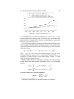
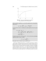
Figure 1.23. Deriving the residual demand curve.
1.3.3.2 The Dominant-Firm Model
The dominant-firm model supposes that there is a monopoly (or collection of firms
acting as a cartel) which is nonetheless constrained to some extent by a competitive
fringe. The central assumption of the model is that the fringe acts in a nonstrategic
manner. We follow convention and develop the model within the context of a price-
setting, single-product monopoly. Dominant-firm models analogous to each of the
cases studied above are similarly easily developed.
If firms which are part of the competitive fringe act as price-takers, they will
decide how much to supply at any given price p. We will denote the supply from
the fringe at any given price p as S
fringe
.p/. Because of the supply behavior of the
fringe, if they are able to supply whomever they so desire at any given price p, the
dominant firm will face the residual demand curve:
D

dominant
.p/ D D
market
.p/  S
fringe
.p/:
Figure 1.23 illustrates the market demand, fringe supply, and resulting dominant-
firm demand curve. We have drawn the figure under the assumption that (i) there
is a sufficiently high price p
1
such that the fringe is willing to supply the whole
market demand at that price leaving zero residual demand for the dominant firm
and (ii) there is analogously a sufficiently low price p
2
below which the fringe is
entirely unwilling to supply.
Given the dominant firm’s residual demand curve, analysis of the dominant-firm
model becomes entirely analogous to a monopoly model where the monopolist faces
the residual demand curve, D
dominant
.p/. Thus our dominant firm will set prices so
60 1. The Determinants of Market Outcomes
that the quantity supplied will equate the marginal revenue to its marginal cost of
supply. That level of output is denoted Q
dominant
in figure 1.23. The resulting price
will be p

and fringe supply at that price is S
fringe

.p

/ D Q
fringe
so that total supply
(and total demand) are
Q
total
D Q
dominant
C Q
fringe
D S
fringe
.p

/ C D
dominant
.p

/ D D
market
.p

/:
A little algebra gives us a useful expression for understanding the role of the fringe
in this model. Specifically, the dominant firm’s own-price elasticity of demand can
be written as
42
Á

dominant
demand
Á
@ ln D
dominant
@ ln p
D
@ ln.D
market
 S
fringe
/
@ ln p
D
1
D
market
 S
fringe
@.D
market
 S
fringe
/
@ ln p
so that we can write
Á
dominant
demand
D

1
D
market
 S
fringe
ÄÂ
D
market
D
market
Ã
@D
market
@ ln p

Â
S
fringe
S
fringe
Ã
@S
fringe
@ ln p

and hence after a little more algebra we have
Á
dominant
demand
D

Â
D
market
D
market
 S
fringe
Ã
@ ln D
market
@ ln p

Â
S
fringe
=D
market
.D
market
 S
fringe
/=D
market
Ã
@ ln S
fringe
@ ln p
D
1
Share

dom
Á
market
demand

Â
Share
fringe
Share
dom
Ã
Á
fringe
supply
;
where Á indicates a price elasticity. That is, the dominant firm’s demand curve—the
residual demand curve—depends on (i) the market elasticity of demand, (ii) the
fringe elasticity of supply, and also (iii) the market shares of the dominant firm and
the fringe. Remembering that demand elasticities are negative and supply elasticities
positive, this formula suggests intuitively that the dominant firm will therefore face
a relatively elastic demand curve when market demand is elastic or when market
demand is inelastic but the supply elasticity of the competitive fringe is large and
the fringe is of significant size.
42
Recall from your favorite mathematics textbook that for any suitably differentiable function f.x/
we can write
@ ln f.x/
@ ln x
D
1

f.x/
@f .x/
@ ln x
:
1.4. Conclusions 61
1.4 Conclusions
 Empirical analysis is best founded on economic theory. Doing so requires
a good understanding of each of the determinants of market outcomes:
the nature of demand, technological determinants of production and costs,
regulations, and firm’s objectives.
 Demand functions are important in empirical analysis in antitrust. The elas-
ticity of demand will be an important determinant of the profitability of price
increases and the implication of those price increases for both consumer and
total welfare.
 The nature of technology in an industry, as embodied in production and
cost functions, is a second driver of the structure of markets. For example,
economies of scale can drive concentration in an industry while economies
of scope can encourage firms to produce multiple goods within a single firm.
Information about the nature of technology in an industry can be retrieved
from input and output data (via production functions) but also from cost, out-
put and input price data (via cost functions) or alternatively data on input
choices and input prices (via input demand functions.)
 To model competitive interaction, one must make a behavioral assumption
about firms and an assumption about the nature of equilibrium. Generally, we
assume firms wish to maximize their own profits, and we assume Nash equi-
librium. The equilibrium assumption resolves the tensions otherwise inherent
in a collection of firms each pursuing their own objectives. One must also
choose the dimension(s) of competition by which we mean defining the vari-
ables that firms choose and respond to. Those variables are generally prices or
quantity but can also include, for example, quality, advertising, or investment

in research and development.
 The two baseline models used in antitrust are quantity- and price-setting mod-
els otherwise known as Cournot and (differentiated product) Bertrand models
respectively. Quantity-setting competition is normally used to describe indus-
tries where firms choose how much of a homogeneous product to produce.
Competition where firms set prices in markets with differentiated or branded
products is often modeled using the differentiated product Bertrand model.
That said, these two models should not be considered as the only models
available to fit the facts of an investigation; they are not.
 An environment of perfect competition with price-taking firms produces the
most efficient outcome both in terms of consumer welfare and production
efficiency. However, such models are typically at best a theoretical abstrac-
tion and therefore they should be treated cautiously and certainly should not
systematically be used as a benchmark for the level of competition that can
realistically be implemented in practice.
2
Econometrics Review
Throughout this book we discuss the merits of various empirical tools that can be
used by competition authorities. This chapter aims to provide important background
material for much of that discussion. Our aim in this chapter is not to replicate the
content of an econometrics text. Rather we give an informal introduction to the tools
most commonly used in competition cases and then go on to discuss the often practi-
cal difficulties that arise in the application of econometrics in a competition context.
Particular emphasis is given to the issue of identification of causality. Where appro-
priate, we refer the reader to more formal treatments in mainstream econometrics
textbooks.
1
Multiple regression is increasingly common in reports of competition cases in
jurisdictions across the world. Like any single piece of evidence, a regression analy-
sis initially performed in an office late at night can easily surge forward and end

up becoming the focus of a case. Once under the spotlight of intense scrutiny,
regression results are sometimes invalidated. Sometimes, it is the data. Outliers or
oddities that are not picked up by an analyst reveal the analysis was performed
using incorrect data. Sometimes the econometric methodology used is proven to
provide good estimates only under extremely restrictive and unreasonable assump-
tions. And sometimes the analysis performed proves—once under the spotlight—to
be very sensitive in a way that reveals the evidence is unreliable. An important part
of the analyst’s job is therefore to clearly disclose the assumptions and sensitivities
at the outset so that the correct amount of weight is placed on that piece of econo-
metric evidence by decision makers. Sometimes the appropriate amount of weight
will be a great, on other occasions it will be very little.
In this chapter we first discuss multiple regression including the techniques known
as ordinary least squares and nonlinear least squares. Next we discuss the important
issue of identification, particularly in the presence of endogeneity. Specifically, we
consider the role of fixed-effects estimators, instrumental variable estimators, and
“natural” experiments. The chapter concludes with a discussion of best practice
1
A very nice discussion of basic regression analysis applied to competition policy can be found in
Fisher (1980, 1986) and Finkelstein and Levenbach (1983). For more general econometrics texts, see, for
example, Greene (2007) and Wooldridge (2007). And for an advanced and more technical but succinct
discussion of the econometric theory, see, for example, White (2001).
2.1. Multiple Regression 63
in econometric projects. The aim in doing so is, in particular, to help avoid the
disastrous scenario wherein late in an investigation serious flaws in econometric
analysis are discovered.
2.1 Multiple Regression
Multiple regression is a statistical tool that allows us to quantify the effect of a
group of variables on a particular outcome. When we want to explain the effect
of a variable on an outcome that is also simultaneously affected by several other
factors, multiple regression will let us identify and quantify the particular effect of

that variable. Multiple regression is an extremely useful and powerful tool but it is
important to understand what it does, or rather what it can and cannot do. We first
explain the principles of ordinary least-squares (OLS) regression and the conditions
that need to hold for it to be a meaningful tool. We then discuss hypothesis testing
and finally we explore a number of common practical problems that are frequently
encountered.
2.1.1 The Principle of Ordinary Least-Squares Regressions
Multiple regression provides a potentially extremely useful statistical tool that can
quantify actual effects of multiple causal factors on outcomes of interest. In an
experimental context, a causal effect can sometimes be measured in a precise and
scientific way, holding everything else constant. For example, we might measure the
effect of heat on water temperature. On the other hand, budget or time constraints
might mean we can only use a limited number of experiments so that each experiment
must vary more than one causal factor. Multiple regression could then be used to
isolate the effects of each variable on the outcomes. Unfortunately, economists in
competition authorities cannot typically run experiments in the field. It would of
course make our life far easier if we could just persuade firms to increase their
prices by 5% and see how many customers they lose; we would be able to learn
about their own-price elasticity of demand relatively easily. On the other hand, chief
executives and their legal advisors may entirely reasonably suggest that the cost of
such an experiment would be overly burdensome on business.
More typically, we will have data that have been generated in the normal course
of business. On the one hand, such data have a huge advantage: they are real! Firms,
for example, will take actions to ameliorate the impact of price increases on demand:
they may invest in customer retention strategies, such as marketing efforts aimed
at explaining to their customers the cost factors justifying a price increase; they
might change some other terms of the offer (e.g., how many weeks of a magazine
subscription you get for a given amount) or perform short-term retention advertising
targeted at the most price-sensitive group of customers. If we run an experiment in a
lab, we will have a “pure” price experiment but it may not tell us about the elasticity of

64 2. Econometrics Review
demand in reality, when real consumers are deciding whether to spend their own real
money given the firm’s efforts at retaining their business. On the other hand, as this
example suggests, a lot will be going on in the real world, and most importantly none
of it will be under the control of the analyst while much of it may be under the control
of market participants. This means that while multiple regression analysis will be
potentially useful in isolating the various causes of demand (prices, advertising,
etc.), we will have to be very careful to make sure that the real-world decisions
that are generating our data do not violate the assumptions needed to justify using
this tool. Multiple regression was, after all, initially designed for understanding data
generated in experimental contexts.
2.1.1.1 Data-Generating Processes and Regression Specifications
The starting point of a regression analysis is the presumption, or at least the hypoth-
esis, that there is a real relationship between two or more variables. For instance, we
often believe that there is a relation between price and quantity demanded of a given
good. Let us assume that the true population relationship between the price charged,
P , and the quantity demanded, Q, of a particular good is given by the following
expression:
2
P
i
D a
0
C b
0
Q
i
C u
i
;

where i indicates different possible observations of reality (perhaps time periods or
local markets) and the parameters a
0
and b
0
take on particular values, for example 5
and 2 respectively. We will call such an expression our “data-generating process”
(DGP). This DGP describes the inverse demand curve as a function of the volume of
sales Q and a time- or market-specific element u
i
, which is unknown to the analyst.
Since it is unknown to the analyst, sometimes it is known as a “shock”; we may call
u
i
a demand shock. The shock term includes everything else that may have affected
the price in that particular instance, but is unknown and hence appears stochastic to
the analyst. Regression analysis is based on the idea that if we have data on enough
realizations of .P; Q/, we can learn about the true parameters .a
0
;b
0
/ of the DGP
without even observing the u
i
s.
If we plot a data set of sample size N , denoted .P
1
;Q
1
/; .P

2
;Q
2
/;:::;.P
N
;Q
N
/
or more compactly f.P
i
;Q
i
/I i D 1;:::;Ng, that is generated by our DGP, we will
obtain a scatter plot with data spread around the picture. An ideal situation for
estimating a demand curve is displayed in figure 2.1. The reason we call it ideal will
become clear later in the chapter but for now note that in this case the true DGP, as
illustrated by the plotted observations, seems to correspond to a linear relationship
2
It is perhaps easier to motivate a demand equation by considering the equation to describe the price
P which generates a level of sales Q.IfQ is stochastic and P is treated as a deterministic “control”
variable, then we would write this equation the other way around. For the purposes of illustration and
since P is usually placed on the y-axis of a classic demand and supply diagram, we present the analysis
this way around, that is, in terms of the “inverse” demand curve.
2.1. Multiple Regression 65
Q
.
.
.
.
.

.
.
.
.
.
.
.
.
.
.
.
.
.
(Q
i
, P
i
)
Q
i
P
i
‘‘Best-fit’’ line
P
Figure 2.1. Scatter plot of the data and a “best-fit” line.
between the two variables. In the figure, we have also drawn in a “best-fit” line, in
this case the line is fit to the data only by examining the data plot and trying to draw
a straight line through the plotted data by hand.
In an experimental context, our explanatory variable Q would often be non-
stochastic—we are able to control it exactly, moving it around to generate the price

variable. However, in a typical economics data set the causal variable (here we are
supposing Q) is stochastic. A wonderfully useful result from econometric theory
tells us that the fact that Q is stochastic does not, of itself, cause enormous problems
for our tool kit, though obviously it changes the assumptions we require for our
estimators to be valid. More precisely, we will be able to use the technique of OLS
regression to estimate the parameters .a
0
;b
0
/ in the DGP provided (i) we consider
the DGP to be making a conditional statement that, given a value of the quantity
demanded Q
i
and given a particular “shock” u
i
, the price P
i
is generated by the
expression above, i.e., the DGP, (ii) we make an assumption about the relationship
between the two causal stochastic elements of the model, Q
i
and u
i
, namely that
given knowledge of Q
i
the expected value of the shock is zero, EŒu
i
j Q
i

 D 0,
and (iii) the sequence of pairs .Q
i
;u
i
/ for i D 1;:::;ngenerate an independent
and identically distributed sequence.
3
The first assumption describes the nature of
the DGP. The second assumption requires that, whatever the level of Q, the average
value of the shock u
i
will always be zero. That is, if we see many markets with
high sales, say of 1 million units per year, the average demand shock will be zero
and similarly if we see many markets with lower sales, say 10,000 units per year,
the average demand shock will also be zero. The third assumption ensures that we
3
Note that the technique does not need to assume that Q and u are fully independent of each other, but
rather (i) that observations of the pairs .Q
1
;u
1
/, .Q
2
;u
2
/, and so on are independent of each other and
follow the same joint distribution and (ii) satisfy the conditional mean zero assumption, EŒu
i
j Q

i
 D 0.
In addition to these three assumptions, there are some more technical “regularity” assumptions that
primarily act to make sure all of the quantities needed for our estimator are finite—see your favorite
econometrics textbook for the technical details.
66 2. Econometrics Review
obtain more information about the process as our sample size gets bigger, which
helps, for example, to ensure that sample averages will converge to their population
equivalents.
4
We describe the technique of OLS more fully bellow. Other estimators
will use different sets of assumptions, in particular, we will see that an alternative
estimation technique, instrumental variable (IV) estimation, will allow us to handle
some situations in which EŒu
i
j Q
i
 ¤ 0.
In most if not all cases, there will be a distinction between the true DGP and the
model that we will estimate. This is because our model will normally (at best) only
approximate the true DGP. Ideally, the model that we estimate includes the true DGP
as one possibility. If so, then we can hope to learn the true population parameters
given enough data. For example, suppose the true DGP is P
i
D 10  2Q
i
C u
i
and the model specification is P
i

D a  bQ
i
CcQ
2
i
Ce
i
. Then we will be able to
reproduce the DGP by assigning particular values to our model parameters. In other
words, our model is more general than the DGP. If on the other hand the true DGP
is
P
i
D 10  5Q
i
C 2Q
2
i
C u
i
and our model is
P
i
D a  bQ
i
C e
i
;
then we will never be able to retrieve the true parameters with our model. In this
case, the model is misspecified. This observation motivates those econometricians

who favor the general-to-specific modeling approach to model specification (see,
for example, Campos et al. 2005). Others argue that the approach of specifying very
general models means the estimates of the general model will be very poor and as
a result the hypothesis tests used to reduce down to more specific models have an
extremely low chance of getting you to the right answer. All agree that the DGP is
normally unknown and yet at least some of its properties must be assumed if we are
to evaluate the conditions under which our estimators will work. Economists must
mainly rely on economic theory, institutional knowledge, and empirical regularities
to make assumptions about the likely true relationships between variables. When
not enough is known about the form of the DGP, one must be careful to either
design a specification that is flexible enough to avoid misspecified regressions or
else test systematically for evidence of misspecification surviving in the regression
equation.
Personally, we have found that there are often only a relatively small number of
really important factors driving demand patterns and that knowledge of an industry
(and its history) can tell you what those important factors are likely to be. By
important factors we mean those which are driving the dominant features of the
data. If those factors can be identified, then picking those to begin with and then
4
The third assumption is often stated using the observed data .P
i
;Q
i
/ and doing so is equivalent
given the DGP. For an introduction to the study of the relationships between the data, DGP, and shocks,
see the Annex to this chapter (section 2.5).
2.1. Multiple Regression 67
refining an econometric model in light of specification tests seems to provide a
reasonably successful approach, although certainly not one immune to criticism.
5

Whether you use a specific-to-general modeling approach or vice versa, the greater
the subtlety in the relationship between demand and its determinants, the better data
you are likely to need to use any econometric techniques.
2.1.1.2 The Method of Least Squares
Consider the following regression model:
y
i
D a C bx
i
C e
i
:
The OLS regression estimator attempts to estimate the effect of the variable x on
the variable y by selecting the values of the parameters .a; b/. To do so, OLS
assigns the maximum possible explanatory power to the variables that we specify as
determinants of the outcome and minimizes the effect of the “leftover” component,
e
i
. The value of the “leftover” component depends on our choice of parameters
.a; b/ so we can write e
i
.a; b/ D y
i
 a  bx
i
. Formally, OLS will choose the
parameters a and b to minimize the sum of squared errors, that is, to solve
min
a;b
n

X
iD1
e
i
.a; b/
2
:
The method of least squares is rather general. The model described above is linear
in its parameters, but the technique can be more generally applied. For example,
we may have a model which is not linear in the parameters which states e
i
.a; b/ D
y
i
f.x
i
Ia; b/, where, for example, f.x
i
Ia; b/ D ax
b
. The same “least-squares”
approach can be used to estimate the parameters by solving the analogous problem
min
a;b
n
X
iD1
e
i
.a; b/

2
:
If the model is linear in the parameters, the technique is known as “ordinary” least
squares (OLS). If the model is nonlinear in the parameters, the technique is called
“nonlinear” least squares (NLLS).
In the basic linear-in-parameters and linear-in-variables model, a given absolute
change in the explanatory variable x will always produce the same absolute change
in the explained variable y. For example, if y
i
D Q
i
and x
i
D P
i
, where Q
i
and
P
i
represent the quantity per week and price of a bottle of milk respectively, then an
increase in the price of milk by €0.50 might reduce the amount of milk purchased by,
say, two bottles a week. The linear-in-parameters and linear-in-variables assumption
implies that the same quantity reduction holds whether the initial price is €0.75 or
€1.50. Because this assumption may not be realistic in many cases, alternative
5
An example of this approach is examined in more detail in the demand context in chapter 9.
68 2. Econometrics Review
Quantity
Price

.
.
.
.
.
ˆ
Residual = Prediction error = P − P
i
a
(Q
i
, P
i
)
Q
i
P
i
OLS estimated mode
ˆ
P
i
ˆ
P
i
= a − bQ
i
ˆ
ˆ
ˆ

Figure 2.2. Estimated residuals in OLS regression.
specifications may fit the data better. For example, it is common to operate a log
transformation on price and quantity variables so that the constant estimated effect
is measured in terms of percentages, y
i
D ln Q
i
and x
i
D ln P
i
. In that case,
@ ln Q
i
=@ ln P
i
D b while @Q
i
=@P
i
D bQ
i
=P
i
so that the absolute changes depend
on the level of both quantity demanded and price. Such variable transformations do
not change the fact that the model is linear in its parameters, and so the model
remains amenable to estimation using OLS.
We first discuss the single-variable regression to illustrate some useful concepts
and results of OLS and then generalize the discussion to the multivariate regression.

First we introduce some terminology and notation. Let . Oa;
O
b/ be estimates of the
parameters a and b. The predicted value of y
i
given the estimates and a fixed value
for x
i
is
Oy
i
DOa C
O
bx
i
:
The difference between the true value y
i
and the estimated Oy
i
is the estimated error,
or the residual e
i
. Therefore, we have
e
i
D y
i
Oy
i

:
Figure 2.2 shows the estimated residuals for our inverse demand curve, where
y
i
D P
i
and x
i
D Q
i
. We see that positive residuals are above the estimated
line and negative residuals are below it. OLS estimation of the inverse demand
curve minimizes the total sum of squares of the “vertical” prediction errors.
6
If the
model nests the true DGP and the parameters of the estimation are exactly right,
then the residuals will be exactly the same as the true “errors,” i.e., the true random
shocks that affect our explained variable.
6
In contrast, if we estimated this model on the demand curve, we would be minimizing the “horizontal”
prediction errors on this graph: imagine rotating the graph in order to flip the axes. The assumptions
required would be different, since they would require, for instance, that EŒe
i
j P
i
 D 0 rather than
EŒe
i
j Q
i

 D 0 and the estimates we obtain will also be different, even if we plot the two lines on the
same graph.
2.1. Multiple Regression 69
Mathematically, finding the OLS estimators involves solving the minimization
problem:
min
a;b
n
X
iD1
e
i
.a; b/
2
D min
a;b
n
X
iD1
.y
i
 a  bx
i
/
2
:
The first-order conditions, also known as the normal equations, are given by setting
the first derivatives with respect to a and b respectively to 0:
n
X

iD1
2.y
i
Oa 
O
bx
i
/.1/ D 0 and
n
X
iD1
2.y
i
Oa 
O
bx
i
/.x
i
/ D 0:
If the model is linear in the parameters, then the minimization problem is quadratic
in the parameters and hence the first-order conditions are linear in the parameters.
As a result, the first-order conditions provide us with a system of linear equations to
solve, one for each parameter. Linear systems of equations are typically often easy to
solve analytically. In contrast, if we write down a nonlinear (in parameters) model,
we may have to solve the minimization problem numerically, but conceptually the
approach is no different.
7
In the two-parameter case, the first normal equation can be solved to give Oa D
Ny 

O
b Nx, where Ny and Nx denote sample averages, as shown below:
n
X
iD1
2.y
i
Oa 
O
bx
i
/.1/ D 0
()
n
X
iD1
y DOan C
O
b
n
X
iD1
x
i
() Oa D
1
n
n
X
iD1

y
i

O
b
1
n
n
X
iD1
x
i
:
The estimated value of the intercept is a function of the other estimated parameter
and the average value of the variables in the regression. If the estimated parameter
O
b is equal to 0 so that our explanatory variables have no explanatory power, then the
estimated parameter Oa (and the predicted value of y) is just the average value of the
dependent variable.
Given the expression for Oa, we can solve
n
X
iD1
2.y
i
Oa 
O
bx
i
/.x

i
/ D 0
()
n
X
iD1
.y
i
Oa 
O
bx
i
/x
i
D 0
7
Programs such as Matlab and Gauss provide a number of standard tools to allow nonlinear problems
to be solved. Solving nonlinear systems of equations can sometimes be very easy in practice, but can also
be very difficult even with the very good computational algorithms now easily accessible to analysts.
70 2. Econometrics Review
()
n
X
iD1
.y
i
 . Ny 
O
b Nx/ 
O

bx
i
/x
i
D 0
()
n
X
iD1
.y
i
Ny/x
i

O
b
n
X
iD1
.x
i
Nx/x
i
D 0
()
O
b D
n
X
iD1

.y
i
Ny/x
i

n
X
iD1
.x
i
Nx/x
i
:
The estimated parameter
O
b is thus the ratio of the sample covariance between the
dependent and explanatory variable (numerator) to the variance of the explanatory
variable (denominator).
More generally, we will want to estimate regression equations where the depen-
dent variable is explained by a number of explanatory variables. For example, sales
may be determined by both price and advertising levels. Alternatively, a “second”
explanatory variable may be a lower- or higher-order term such as a square root
or squared term meaning that such a specification can account for both multi-
ple variables and also particular types of nonlinearities in variables. Retaining the
linear-in-parameters specification, a multivariate regression equation takes the form:
y
i
D a C b
1
x

1i
C b
2
x
2i
C b
3
x
3i
C e
i
:
For given parameter values, the predicted value of y
i
for given estimates and values
of .x
1i
;x
2i
;x
3i
/ is
Oy
i
DOa C
O
b
1
x
1i

C
O
b
2
x
2i
C
O
b
3
x
3i
and so the prediction error is e
i
D y
i
Oy
i
.
In this case, the minimization problem is the same as the case with two parameters
except that it involves more parameters to minimize over:
min
a;b
1
;b
2
;b
3
n
X

iD1
e
i
.a; b
1
;b
2
;b
3
/
2
:
Fortunately, as in the two-parameter case, provided the model is linear in the param-
eters this minimization problem is a quadratic program and so will have first-order
conditions which are also linear in the parameters and admit analytic solutions.
To find those solutions, however, it is usually easier to use matrix notation, fol-
lowing the unifying treatment provided by Anderson (1958). To do so, simply stack
up observations for the regression equation above to define the equivalent matrix
expression
2
6
6
6
6
4
y
1
y
2
:

:
:
y
n
3
7
7
7
7
5
D
2
6
6
6
6
4
1x
11
x
21
x
31
1x
12
x
22
x
32
:

:
:
:
:
:
:
:
:
:
:
:
1x
1n
x
2n
x
3n
3
7
7
7
7
5
2
6
6
6
4
a
b

1
b
2
b
3
3
7
7
7
5
C
2
6
6
6
6
4
e
1
e
2
:
:
:
e
n
3
7
7
7

7
5
D
2
6
6
6
6
4
x
0
1
x
0
2
:
:
:
x
0
n
3
7
7
7
7
5
ˇ C
2
6

6
6
6
4
e
1
e
2
:
:
:
e
n
3
7
7
7
7
5
;
2.1. Multiple Regression 71
which can in turn be more simply expressed in terms of vectors and matrices as
y D Xˇ C e;
where y is an .n 1/ vector and X is an .nk/ matrix of data, while ˇ is the .k 1/
vector of parameters to be estimated and e is the .n 1/ vector of residuals. In our
example, k D 4 as there are four parameters to be estimated.
The general OLS minimization problem can be easily solved by using matrix
notation. Specifically, note that the OLS minimization problem can be expressed
as
min

ˇ
e.ˇ/
0
e.ˇ/ D min
ˇ
.y  Xˇ/
0
.y  Xˇ/;
so that the k first-order conditions are the (linear-in-parameters) form:
@.y  Xˇ/
0
.y  Xˇ/
@ˇ
D 2.X/
0
.y  Xˇ/
D 2.X
0
y C X
0
Xˇ/
D 0:
Solving for the vector of coefficients ˇ, we obtain the general formula for the OLS
regression estimator in the multivariate case:
O
ˇ
OLS
D .X
0
X/

1
X
0
y:
Note that this formula is the multivariate equivalent of the bivariate results we
developed earlier.
The variance of the OLS estimator can be calculated as follows:
Var Œ
O
ˇ
OLS
j X D EŒ.
O
ˇ
OLS
 EŒ
O
ˇ
OLS
j X/.
O
ˇ
OLS
 EŒ
O
ˇ
OLS
j X/
0
j X:

Now if we suppose that the DGP is of the form y D Xˇ
0
C u, then
EŒ
O
ˇ
OLS
j X D EŒ.X
0
X/
1
X
0
.Xˇ
0
C u/ j X
D ˇ
0
C .X
0
X/
1
X
0
EŒu j X
D ˇ
0
:
Provided EŒu j X D 0 and since
O

ˇ
OLS
 ˇ
0
D .X
0
X/
1
X
0
u,wehave
Var Œ
O
ˇ
OLS
j X D EŒ.X
0
X/
1
X
0
u X
0
X/
1
X
0
u/
0
j X

D .X
0
X/
1
X
0
.EŒuu
0
j X/X.X
0
X/
1
:
If the variance is homoskedastic so that EŒuu
0
j X D 
2
I
n
, then the formula
collapses to the simpler expression,
Var Œ
O
ˇ
OLS
j X D .X
0
X/
1


2
I
n
:
72 2. Econometrics Review
2.1.2 Properties of OLS
Ordinary least squares is a simple and intuitive method to apply, which explains some
of its popularity. However, it is also attractive because the estimators it produces
exhibit some very desirable properties provided the assumptions it requires hold.
Next we briefly review these properties and the conditions necessary for them to
hold.
2.1.2.1 Unbiasedness
An estimator is unbiased if its expected value is equal to the true value, i.e., if the
estimator is “on average” the true value. This means that the average of the coefficient
estimates over all possible samples of size n, f.X
i
;Y
i
/I i D 1;:::;ng, would be
equal to the true value of the coefficient. Formally,
EŒ
O
ˇ D ˇ
0
;
where ˇ
0
is the true parameter of the DGP. The unbiasedness property is equivalent to
saying that, on average, OLS estimation will give us the true value of the coefficient.
For OLS estimators to be unbiased, a largely sufficient condition

8
given the DGP
y D Xˇ
0
C u is that EŒu j X D 0, meaning that the real error term must be
unrelated to the value of our explanatory variables. For instance, if we are explaining
the quantity demanded as a function of price and income, it is necessary that the
shocks to the demand be uncorrelated with the level of prices or income.
The unbiasedness condition can formally be obtained by applying the law of iterative
expectations that states that the expected value of a variable is equal to the expected
value of the conditional expectation over the whole set of possible values of the
conditions. Formally, it states that EŒ
O
ˇ
OLS
 D E
X
ŒEŒ
O
ˇ
OLS
j X. This allows us to
write the expected value of the OLS estimator as follows:
EŒ
O
ˇ
OLS
j X D .X
0
X/

1
X
0
EŒy j X D .X
0
X/
1
X
0
EŒXˇ
0
C u j X
D .X
0
X/
1
X
0
Xˇ
0
C .X
0
X/
1
X
0
EŒu j X
D ˇ
0
C 0 if EŒu j X D 0:

In general, unbiasedness is a tougher requirement than consistency, which we
discuss next. In particular, while we will typically be able to find estimators for
linear models which are both unbiased and also consistent, many nonlinear models
will admit estimators which are consistent but not unbiased.
8
Strictly, there are in fact other regularity conditions which together suffice. In particular, we will
require that .X
0
X=n/
1
exists.
2.1. Multiple Regression 73
2.1.2.2 Consistency
An estimator is a consistent estimator of a parameter if it tends toward the true
population value of the parameter as the sample available for estimation gets large.
The property of consistency for averages is derived from a “law of large numbers.” A
law of large numbers provides a set of assumptions under which a statistic converges
to its population equivalent. For example, the sample average of a variable will
converge to the true population average as the sample gets big under weak conditions.
Somewhat formally, we can write one such law of large numbers as follows. If
X
1
;X
2
;:::;X
n
is an independent random sample of variables from a population
with mean <1 and variance 
2
< 1 so that EŒX

i
 D  and VarŒX
i
 D 
2
,
then consistency means that as the sample size n gets bigger the sample average
converges
9
to the population average:
N
X
n
D
1
n
n
X
iD1
X
i
! :
Note that the necessary conditions for this to happen are that the first and second
moments, i.e., the mean and the variance, of the variable exist and are finite. Those
are relatively weak requirements as they will tend to hold in the case of almost all
economic variables, which generally have a finite range of possible values.
10
Let us develop the requirements for consistency of OLS. To do so, write the OLS
estimator as
O

ˇ
OLS
D .X
0
X/
1
X
0
y
D .X
0
X/
1
X
0
.Xˇ
0
C u/
D ˇ
0
C .X
0
X/
1
X
0
u:
We have
O
ˇ

OLS
D ˇ
0
C
Â
X
0
X
n
Ã
1
Â
1
n
X
0
u
Ã
:
Note that each of the terms in X
0
X=n and .1=n/X
0
u are actually just sample aver-
ages. The former has, as its jkth element, .1=n/
P
n
iD1
x
ij

x
ik
while the latter has, as
its j th element, .1=n/
P
n
iD1
x
ij
u
i
. These are just sample averages which, accord-
ing to a “law of large numbers,” will converge to their respective population means.
9
Econometrics textbooks will often spend a considerable amount of time defining precisely what we
mean by “converge.” The two most common concepts are “convergence in probability” and “almost sure
convergence.” These respectively provide the “weak” law of large numbers and the “strong” law of large
numbers (SLLN).
10
A random variable which can only take on a finite set of values (technically, has finite support) will
have all moments existing. Possible exceptions (might) be price data in hyperinflations, where prices can
go off to close to infinity in extreme cases but even there presumably there is a limit on the amount of
money that can be printed and also on the number of zeros that can be printed on any piece of paper. In
contrast, occasionally economic models of real world quantities do not have finite moments. For example,
Brownian motions are sometimes used in finance as approximations to the real world.
74 2. Econometrics Review
We also require that inverting the matrix .X
0
X=n/
1

does not cause any problems
(e.g., division by zero would be bad). In fact, the OLS estimator will be consistent
if, for a large enough sample,
(1)
X
0
X
n
! M
X
, where M
X
is a positive definite .k  k/ matrix;
(2)
X
0
u
n
! 0
,a.k  1/ vector of zeros.
In each case, we will require laws of large numbers to hold. That will mean we
will require finite first and second moments with, in the case of (2), the first popu-
lation moment equal to zero. Thus the assumptions required for OLS to converge
will involve those which ensure a law of large numbers to hold and then assump-
tions on the population averages. Specifically, that EŒu
i
x
ij
 D 0 or, because of
the law of iterated expectations, it suffices to assume that EŒu

i
j x
ij
 D 0 since
E
.u;x/
Œu
i
x
ij
 D E
x
Œ.E
ujx
Œu
i
j x
ij
/x
ij
 D E
x
Œ.0/x
ij
 D 0.
It should by now be clear that our assumption EŒu
i
j x
ij
 D 0 plays a central role

in ensuring OLS is consistent. If this assumption is violated, OLS estimation may
well produce estimators that bear no relation to the true value of the parameters of
the DGP, even if we fortuitously write down a family of models which includes the
DGP. Unfortunately, this crucial assumption is often violated in real world settings.
Among others, causes can include (i) misspecification of models, (ii) measurement
error, and (iii) endogeneity.We discuss these problems, and in particular the problem
of endogeneity, later in this chapter.
2.1.3 Hypothesis Testing
Econometric estimation produces an estimate of one or more parameters. A sample
will provide an estimate, not the population value. Hypothesis testing involving a
parameter helps us measure the extent to which the estimated outcome is consistent
with a particular assumption about the real magnitude of the effect. In terms of a
parameter, the hypothesis could be that the parameter takes on a particular value,
say 1.
11
Concretely, hypothesis testing helps us explicitly reject or not reject a given
hypothesis with a specified degree of certainty—or “confidence.” To understand
how this is done, we need to understand the concept of confidence intervals.
11
More generally, we can test whether the assumptions required for our model and econometric esti-
mator are in fact satisfied. In terms of a model, the hypothesis could be that a model is correctly specified
(see, for example, any econometric text’s discussion of the RESET test). In terms of an estimator, the
hypothesis could be that an efficient estimator that requires strong assumptions is consistent and the
strong assumptions are true (see any econometric discussion of the Wu–Durbin–Hausman test).
2.1. Multiple Regression 75
Density
jjj
σβ
2
0

−
)|
ˆ
( X
f
j
β
jjj
σβ
−
0
jjj
σβ
+
0
jjj
σβ
2
0
+
j
β
ˆ
j0
β
√
√
√
√
Figure 2.3. The distribution of an OLS estimator:

EŒ
O
ˇ
j
j X D ˇ
0j
and VarŒ
O
ˇ
j
j X D 
jj
.
2.1.3.1 Measuring Uncertainty and Confidence Intervals
OLS regressions produce estimates for the parameters of our specified model by
using the information given by the sample data, and as a result the parameter esti-
mates from an OLS regression are stochastic variables. Estimates are normally based
on a sample of the population, not on the entire population. That means that if we
had drawn a different sample, we would probably have obtained different estimates.
The unbiasedness property of our OLS estimator tells us that the expected value
of our estimated coefficient is the true value of the parameter, EŒ
O
ˇ
j
j X D ˇ
0j
,
where “j” denotes the j th element of the parameter vector ˇ. Recall also that
we can measure the level of uncertainty attached to any estimated coefficient by
evaluating its standard deviation, normally called the standard error in this context.

Defining VarŒ
O
ˇ
j
j X D 
jj
, we can write s: e:Œ
O
ˇ
j
j X D
p

jj
. By estimating ˇ
j0
with different samples of size n, we would end up with a distribution of realized
values of the estimator such as that shown in figure 2.3.
In any given sample, we can construct estimates of ˇ
0j
and 
jj
, so that we can
obtain information about the distribution of the estimator, even though we only
have one sample. Estimating the distribution gives us an idea of how different the
estimator could be if we drew a different sample of the same size. If the estimator
has a normal distribution (as statistical theory often tells us, it would eventually—if
our estimator satisfies a suitable central limit theorem), then 95% of the distribution
density will lie within two standard errors of the mean.
12

This means that for 95%
of the samples of a given size, the estimator would fall within that interval. Such an
interval is called the “95% confidence interval” since we are 95% confident that our
estimator would fall within that range.
12
See, for example, chapter 5 of White (2001) for the conditions under which OLS estimators will
satisfy a central limit theorem. Note that introductory texts often talk about “the” central limit theorem
(CLT), whereas in truth CLTs are a type of theorem and there are many of them; for instance, not all
CLTs involve normal distributions.
76 2. Econometrics Review
2.1.3.2 Hypothesis Testing
Hypothesis testing is important in econometrics and it involves testing an assump-
tion referred to as the “null hypothesis” against an alternative creatively called the
“alternative hypothesis.” The most common test for an estimator is the test to see
whether the estimator is statistically “significant,” meaning significantly different
from zero. In that case the null hypothesis to be tested is written as
H
0
W ˇ
0
D 0
while the alternative hypothesis could be written as
H
10
W ˇ
0
D ˇ
alt
:
We want to test whether we can reject the null hypothesis with sufficient confidence.

If the null hypothesis is true, the expected value of the estimated parameter is 0 and
therefore in 95% of cases (samples drawn from the population) the estimated value
for the parameter will fall within the 95% confidence interval given by .2
ˇ
;2
ˇ
/.
Generally, we consider that falling outside of the 95% confidence interval is unlikely
enough (it happens only 5% of the time) to allow us to reject that the null hypothesis
is true. Careful analysts will describe such a hypothesis test as having provided
an answer with 95% confidence and may also go on to consider whether we can
reject the null hypothesis with 99% or higher confidence. Analogously, under the
alternative hypothesis that ˇ
0
is some nonzero value ˇ
alt
, estimating the parameter
value to be zero or close to zero will occur with certain probability. We need to assess
whether the probability of finding a zero estimate if the alternative hypothesis is true
is low enough to let us reject the assumption that the true value is ˇ
alt
. Figure 2.4
illustrates graphically the values of the estimator for which we would reject or fail
to reject that the true value of the coefficient is 0.
Figure 2.4 also illustrates two very important concepts in hypothesis testing, both
of which have important implications for policy making. Specifically, since our test
relies on some measure of probability, making an error in rejecting or accepting a
hypothesis is always a possibility. There are two types of errors, helpfully known as
“type I” and “type II”:
Type I. An analyst may reject the null hypothesis when it is, in fact, true. This is

called making a type I error. We will make type I errors 5% of the time when using
a 95% level test (one in twenty tests). In figure 2.4 the probability of making a
type I error is depicted by the lighter area plus the area to the left of 2
ˇ
.
Type II. Alternatively, we can fail to reject our null hypothesis when it is actually
false. This is called making a type II error. It is more difficult to know how likely
this error is since it will depend on how close the true value of the parameter (let
us say ˇ
alt
in figure 2.4) is to the null hypothesis. In figure 2.4 this probability is
depicted by the darker area, which is the area within the 95% confidence interval
of the null hypothesis.
2.1. Multiple Regression 77
0
= 0
+2
=
Accept H
0
Density under
the null hypothesis
Trade-off in types
can be seen by moving
the critical region
for acceptance/ rejection
Density under
alternative
hypothesis
β

σ
−
2
β
σ
β
β
0
β
alt
)
|
(f
β
H
0
)
|
(f
β
H
1
Type II error
Type I error
Reject H
0
Figure 2.4. Hypothesis testing and the trade-off between type I and type II errors.
Both type I and II errors are undesirable but also unavoidable without collecting
more information. Assume that our null hypothesis is that a parameter indicating
some kind of competitive abuse is zero. For example, this could be a parameter

indicating a cartel overcharge. With a null hypothesis of innocence, a type I error
will mean that we decide that there was an abuse when in fact there was none
(we find an innocent company guilty). A type II error means that we determine
that there was no abuse when in fact there was abuse (we find a guilty company
innocent). A decision rule will always have implications for the probability of those
two kinds of errors and both errors can be costly. For instance, finding predation
when there was none will have the effect of raising prices and may actively impede
effective competition that was beneficial for consumers. On the other hand, if we
find that prices are competitive when in truth there was predation, we may disturb
the competitive process by permitting such foreclosure strategies. Whether we make
the type I or the type II error large will therefore be a policy choice. We might decide
to apply a criminal standard that “it is better that twelve guilty men go free than an
innocent goes to jail,” a standard which makes the type I error small but in doing
so makes the type II error large. In the figure this trade-off can be seen by moving
the critical region for acceptance or rejection; shrinking the type I error makes the
type II error larger. Some note that in competition analysis if the hypothesis that
a firm is abusing its market power is incorrectly rejected by a competition agency,
then the forces of competition may nonetheless correctly redress the error while
interventions by government, perhaps in the form of regulation, may persist far
78 2. Econometrics Review
longer. Ultimately, the question of the relative size of forces working to correct the
system after an error of regulatory judgment, and hence the relative costs of such
policy errors, is an empirical question. However, it is probably fair to say that it is
an important empirical question on which there is not a great deal of hard empirical
evidence.
13
2.1.3.3 The t-Test
The t-test is the test used to consider the null hypothesis that H
0
W ˇ

0j
D 0 when
evaluating OLS coefficient estimates. Specifically, suppose our estimate for the true
parameter ˇ
0j
associated with the j th regressor is
O
ˇ
0j
. We may want to know
whether we can reject the hypothesis that the value of the true parameter is 0.
If the value 0 falls within the 95% confidence interval constructed using
O
ˇ
0j
and
its standard error s: e:.
O
ˇ
j
/, then we will not be able to reject the hypothesis that the
true value is 0 because the realized value of
O
ˇ
0j
is not unlikely enough if 0 was
indeed the true magnitude of the effect. If performing a 95% test of significance, we
will reject the null hypothesis that the true parameter is equal to a given value if that
value falls outside of the 95% confidence interval of the estimated parameter
O

ˇ
0j
.
The standard way to test the null hypothesis that the true parameter ˇ
0j
is in fact
a particular number ˇ
j
(e.g., zero), H
0
W ˇ
0j
D ˇ
j
, is to compute a statistic called
the “t-statistic,” which takes the following form (Student 1908)
14
:
t Á
O
ˇ
j
 ˇ
j0
s.e
O
ˇ
j
/
:

The t -statistic calculates the difference between the estimator and the value proposed
as the null hypothesis value and expresses it as a proportion of the standard deviation
of the estimator (its standard error), s.e. .
O
ˇ
j
/ D
p
Var .
O
ˇ
j
/.
15
Testing whether the
null hypothesis is true is equivalent to testing whether the t-statistic is equal to 0.
Under standard assumptions, a t-statistic has a probability distribution called
Student’s t-distribution. For large samples, this distribution approaches the normal
distribution and in this case any t value higher than 1.96 in absolute value will have a
13
That said, collecting more information can reduce both type I and type II errors in any given situation.
To see why, consider what would happen in figure 2.4 if the variance of the distributions shrinks. With
more information, the chance of a type II error falls for a given level of type I error and, also, we
can typically reduce type I errors because more data allow higher confidence levels to be used. More
information is, however, not a panacea in reality since collecting it costs money. If the burden of evidential
proof required of a competition agency on a given case is high, then competition agencies with limited
budgets will prioritize their casework. Doing so means reducing the number of cases investigated. That
in turn affects the chance of prosecution and hence reduces deterrence. As a result, and quite probably
only in principle rather than practice, the optimal size of a competition agency’s budget will depend on
all these factors.

14
The development of the t-distribution involved important contributions from Student (actually a
pseudonym for Gosset) and Fisher (1925). Their respective contributions are described in Fisher-Box
(1981).
15
For example, for an OLS estimator we have derived the formula: Var.
O
ˇ
j
/ D 
2
.X
0
X/
1
2.1. Multiple Regression 79
probability of less than 5% if the null hypothesis involves ˇ
0j
D 0.
16
So, in practice,
we reject the null hypothesis ˇ
0j
D 0 when the absolute value of the t-statistic is
higher than 1.96. Since 2 is, for most practical purposes, sufficiently close to 1.96,
as a rule of thumb and for a quick first look, if the estimated coefficient
O
ˇ
j
is more

than double its standard error, the null hypothesis that the true value of the parameter
is 0 can be rejected and
O
ˇ
j
is said to be significantly different from 0. In general,
small standard errors and/or a big difference between the value of the parameter
under the null hypothesis and the estimated coefficient will mean that we reject the
null hypothesis.
To illustrate let us use the Hausman et al. (1994) demand estimates, presented
in table 2.1. The first column of results represents the parameters of an equation
characterizing the demand for Budweiser beer.
17
Let us test whether we can reject
the hypothesis that the coefficient of the log of price of Budweiser in that equation
is equal to zero. The t-statistic will be
t D
O
ˇ
j
 ˇ
j0
p
O
jj
D
0:936  0
0:041
D22:8:
Since jtjD22:8 > 1:96 we can easily reject the null hypothesis that the effect of

the price of Budweiser on the quantity demanded for Budweiser is 0 with a 95%
degree of confidence. In fact, with a t -statistic of 22.8 we could easily also reject
the null hypothesis with a 99% degree of confidence.
2.1.4 Common Problems in Multiple Regressions
Running a regression in a statistical package is extremely simple given modern user-
friendly software and fast computers. The results can also often be intuitive. Partly
as a result of such progress, the use of regression analysis has become very common
in competition policy, as in many other fields. In terms of generating output—
“numbers”—OLS and other estimators like instrumental variables (IVs) are very
simple to implement, and are potentially very powerful tools.Yet estimators like OLS
and IVs rely on strong underlying assumptions, assumptions which are frequently
likely to be violated in many economic contexts. As a result, using econometrics to
develop numbers that one can confidently “believe” remains a highly skilled job.
Weeding out unreliable regression results is easier but even that is not without serious
challenges.
A set of regression estimates are only as good as the underlying assumptions
used to build and estimate the model. Basically, there are two types of assumptions.
First, given a regression model, say a linear regression model, there are econometric
16
For very small samples, a table indicating the probability distribution of the t-statistic can be used.
Such tables are generally available in econometrics books.
17
In fact these equations are “brand share” equations. We will consider the equations in more detail in
chapter 9.
80 2. Econometrics Review
Table 2.1. Estimation for the demand for premium
beer brands (symmetry imposed during estimation).
12345
Budweiser Molson Labatts Miller Coors
Constant 0.393 0.377 0.230 0.104 —

(0.062) (0.078) (0.056) (0.031) —
Time 0.001 0.000 0.001 0.000 —
(0.000) (0.000) (0.000) (0.000) —
log.Y =P / 0.004 0.011 0.006 0.017 —
(0.006) (0.007) (0.005) (0.003) —
log.P
Budweiser
/ 0.936 0.372 0.243 0.150 —
(0.041) (0.231) (0.034) (0.018) —
log.P
Molson
/ 0.372 0.804 0.183 0.130 —
(0.231) (0.031) (0.022) (0.012) —
log.P
Labatts
/ 0.243 0.183 0.588 0.028 —
(0.034) (0.022) (0.044) (0.019) —
log.P
Miller
/ 0.150 0.130 0.028 0.377 —
(0.018) (0.012) (0.019) (0.017) —
log(number of stores) 0.010 0.005 0.036 0.022 —
(0.009) (0.012) (0.008) (0.005) —
Conditional own 3.527 5.049 4.277 4.201 4.641
Price elasticity (0.113) (0.152) (0.245) (0.147) (0.203)
˙ D
8
ˆ
ˆ
<

ˆ
ˆ
:
0:000359 1:436  10
5
0:000158 2:402  10
5
0:000109 6:246  10
5
1:847  10
5
0:005487 0:000392
0:000492
9
>
>
=
>
>
;
Source: Hausman et al. (1994).
assumptions required to estimate it. In the heat of a case, sometimes staff economists
are tempted to remember the appealing properties of OLS estimators while the
assumptions that generate those appealing features are, shall we say, less clearly at
the forefront of analytical working papers.
Secondly, there are assumptions that generate a given regression model. Even
when no economic model has been explicitly used to derive the form of the regres-
sion, the regression will always correspond to a particular implicit model or a family
of economic models. Naturally, if the implicit model is materially wrong it may not
be appropriate to rely on the regression results. If we do not state the assumptions

explicitly, then the interpretation of regression results becomes even harder since
the reader (perhaps the judge in a case context) must figure out what those assump-
tions are and whether they are reasonable. On the other hand, if we state all of our
assumptions up-front, we need to be sure that such overt honesty is not inappro-
priately punished by either the courts of public opinion or whichever judicial body
reviews an agency’s competition decision. To make any progress in analysis we may
2.1. Multiple Regression 81
have to pick the least undesirable set of assumptions. Of course, every model of the
world is inevitably “wrong,” and such issues often require quite careful judgment
in light of all the evidence available in a given case. On other occasions, formal
statistical methods can help inform such judgments powerfully. For example, when
the data we have can reject the model we are positing as being the true DGP.
In this section, we will describe the most common problems found to occur
during the implementation of regression analysis and outline the ways the literature
has attempted to address them. Specifically, we discuss in turn misspecification,
endogeneity, multicollinearity, measurement error, and heteroskedasticity.
2.1.4.1 Misspecification
Generally, misspecification occurs when a regression model cannot represent, for
any value of the parameters, the true data-generating process (DGP). In other words,
the econometric model is not a valid representation of the process in the world which
generates the data. This happens because the regression model specified by the
analyst has imposed restrictions on the relationship between the variables that is not
true. As we have noted, in reality no model is “correctly specified” but, nonetheless,
testing to see whether the data we have clearly reject the model we are working with
in favor of a more appropriate one is a very useful and important activity. This kind
of specification error can result from the imposition of an incorrect functional form
in the relation between two variables when the true relationship is nonlinear. For
example, we may have included the wrong variable specification in a regression,
perhaps x instead of ln.x/.
Another source of specification error can be the omission of an important explana-

tory variable, a source of error which is equivalent to forcibly setting its coefficient
in the regression to zero. For example, we may have omitted a term with a higher
order such as the squared value of a regressor. Misspecification due to an erroneous
functional form can produce biased estimates. The cost estimation in Nerlove (1963)
discussed in chapter 3 presents an illustration of this problem, and its solution.
18
If
the omitted variable is important to explain our dependent variable and if it hap-
pens to be also correlated with one of the explanatory variables included in the
regression, the estimated parameters on the included regressors in our regression
will be biased. This problem of “omitted variables” can be considered to be one
source of the problem of endogeneity, a problem we discuss below. If the omitted
variables are not correlated with any of the other of the regressors, then the problem
is not immediately serious since the estimators will often be unbiased. That said,
we will get a lower level of explanatory power in our model than if we included all
the relevant variables. A very low explanatory power, as represented by a very low
R-squared, is a sign that we are missing important determinants of our explained
18
See the practical examples in chapter 3 for a discussion of the Nerlove (1963) paper.
82 2. Econometrics Review
outcome.
19
This is not always a problem—for example, if we are only interested
in the value of a particular coefficient and we are confident that the error term, i.e.,
what is left out, is uncorrelated with any of our included regressors. On the other
hand, if we are trying to model the explained variable, a very low R-squared can
be an indication that we are missing important determinants and therefore that our
model of the data-generating process is substantially incomplete.
Alternatively, misspecification can result from the omission of an interaction term
between variables when the true value of a coefficient is dependent on the level of

another one of the variables. For instance, the effect of a price increase on quantity
demanded might depend on people’s level of income. Interactions might be a good
idea when the effect of a variable is measured over a very wide range of the values
of the remaining regressors since in that case nonlinearities are more likely to occur.
In some cases, misspecification can be detected by informally checking the behav-
ior of the estimated error term, the residuals. For example, sometimes plotting the
residuals versus the explanatory variables reveals some systematic patterns between
them. If so, the OLS assumption that EŒu
i
j x
i
 D 0 is probably violated and the
estimates biased. More formally, an econometric literature has evolved to exam-
ine specification issues. If the null hypothesis of misspecification can be stated as
a parametric restriction on a more general alternative model (e.g., a model with
both x and ln.x/), then we can use classical tests to evaluate misspecification (see
Godfrey 1989).
20
An early and yet still very useful test for general functional form
misspecification is provided by Ramsey (1969).
2.1.4.2 Endogeneity
Endogeneity of regressors is probably the argument used most frequently to raise
concerns about regression analyses. The reason is that potential endogeneity prob-
lems tend to be pervasive in economics and the solutions to endogeneity problems
are sometimes few and far between. As a result, endogeneity is sometimes inap-
propriately ignored even though it can fatally invalidate the results of a regression.
Endogeneity means that one of the regressors used in the model is correlated with
the “shock” component of the model.
One reason for such a correlation is if we are suffering from an omitted-variable
problem (see above). For example, an included regressor might be entirely irrele-

vant but correlated (for whatever reason) with the true causal factor, which has been
19
Or in the case of IV regression a suitably adjusted R-squared.
20
Recall that the classical trinity of statistical tests states that you can fit either (1) the unrestricted
model and test whether the restrictions are rejected (e.g., true parameters are zero), (2) the restricted model
and test whether the derivative of the objective function (e.g., likelihood) with respect to a parameter
is nonzero when evaluated at a parameter value associated with the restricted model (usually zero), or
(3) the likelihood ratio approach, which involves fitting both the restricted and unrestricted models. These
three approaches are known as the Wald, the Lagrange multiplier, and the likelihood ratio approaches,
respectively.