Quantitative Techniques for Competition and Antitrust Analysis_1 pdf

Quantitative Techniques for
Competition and Antitrust Analysis
This page intentionally left blank
Quantitative Techniques for
Competition and Antitrust Analysis
Peter Davis and Eliana Garc´es
Princeton University Press
Princeton and Oxford
Copyright
c
 2010 by Peter Davis and Eliana Garc´es
Requests for permission to reproduce material from this work
should be sent to Permissions, Princeton University Press
Published by Princeton University Press,
41 William Street, Princeton, New Jersey 08540
In the United Kingdom: Princeton University Press,
6 Oxford Street, Woodstock, Oxfordshire OX20 1TW
All Rights Reserved
Library of Congress Cataloging-in-Publication Data
Davis, Peter J. (Peter John), 1970–
Quantitative techniques for competition and antitrust analysis / Peter Davis, Eliana Garc´es.
p. cm.
Includes bibliographical references and index.
ISBN 978-0-691-14257-9 (alk. paper)
1. Consolidation and merger of corporations. 2. Antitrust law.
3. Econometrics. I. Garc´es, Eliana, 1968– II. Title.
HD2746.5.D385 2010
338.8
0
2015195–dc22 2009005675

British Library Cataloging-in-Publication Data is available
This book has been composed in Times using T
E
X
Typeset and copyedited by T
&
T Productions Ltd, London
Printed on acid-free paper.
∞
press.princeton.edu
Printed in the United States of America
10987654321
For Lara, Adrian, and Tristan
For Sara
This page intentionally left blank
Contents
Preface ix
Acknowledgments xii
1 The Determinants of Market Outcomes 1
1.1 Demand Functions and Demand Elasticities 1
1.2 Technological Determinants of Market Structure 19
1.3 Competitive Environments: Perfect Competition, Oligopoly, and
Monopoly 37
1.4 Conclusions 61
2 Econometrics Review 62
2.1 Multiple Regression 63
2.2 Identification of Causal Effects 89
2.3 Best Practice in Econometric Exercises 113
2.4 Conclusions 119
2.5 Annex: Introduction to the Theory of Identification 121

3 Estimation of Cost Functions 123
3.1 Accounting and Economic Revenue, Costs, and Profits 125
3.2 Estimation of Production and Cost Functions 131
3.3 Alternative Approaches 149
3.4 Costs and Market Structure 158
3.5 Conclusions 160
4 Market Definition 161
4.1 Basic Concepts in Market Definition 162
4.2 Price Level Differences and Price Correlations 169
4.3 Natural Experiments 185
4.4 Directly Estimating the Substitution Effect 191
4.5 Using Shipment Data for Geographic Market Definition 198
4.6 Measuring Pricing Constraints 201
4.7 Conclusions 227
viii Contents
5 The Relationship between Market Structure and Price 230
5.1 Framework for Analyzing the Effect of Market Structure on Prices 231
5.2 Entry, Exit, and Pricing Power 256
5.3 Conclusions 282
6 Identification of Conduct 284
6.1 The Role of Structural Indicators 285
6.2 Directly Identifying the Nature of Competition 300
6.3 Conclusions 341
6.4 Annex: Identification of Conduct in Differentiated Markets 343
7 Damage Estimation 347
7.1 Quantifying Damages of a Cartel 347
7.2 Quantifying Damages in Abuse of Dominant Position Cases 377
7.3 Conclusions 380
8 Merger Simulation 382
8.1 Best Practice in Merger Simulation 383

8.2 Introduction to Unilateral Effects 386
8.3 General Model for Merger Simulation 401
8.4 Merger Simulation: Coordinated Effects 426
8.5 Conclusions 434
9 Demand System Estimation 436
9.1 Demand System Estimation: Models of Continuous Choice 437
9.2 Demand System Estimation: Discrete Choice Models 462
9.3 Demand Estimation in Merger Analysis 491
9.4 Conclusions 499
10 Quantitative Assessment of Vertical Restraints and Integration 502
10.1 Rationales for Vertical Restraints and Integration 503
10.2 Measuring the Effect of Vertical Restraints 518
10.3 Conclusions 553
Conclusion 555
References 557
Index 577
Preface
The use of quantitative analysis by competition authorities is increasing around the
globe. Whether the quantitative analysis is submitted by external experts, or the com-
petition authority itself undertakes the analysis, empirical analysis is now a vitally
important component of the competition economist’s toolkit. Much of the empiri-
cal analysis submitted to, or carried out by, investigators is fairly straightforward.
This is partly because simple tools are often very powerful and partly because the
need to communicate with nonexperts sometimes places a natural boundary on the
degree of sophistication which can comfortably be used. Of course, one person’s
“cutting-edge” method is another’s basic tool and this difference drives the normal
process of diffusion of new methods from basic research to applied work. The tools
we discuss in this book are broadly the result of the ideas and methods which have
developed over the past twenty years in the empirical industrial organization liter-
ature and which are either gradually diffusing into practice or, no doubt in a small

number of cases, gradually diffusing into obscurity.
While the aim of this book is to examine empirical techniques, we cannot stress
enough that any empirical analysis in a competition investigation needs to be eval-
uated together with the factual, documentary, and qualitative evidence collected
during the case. An empirical analysis will usually be one albeit important element
in a broader evidence base. Only in a small minority of cases will quantitative analy-
sis alone be sufficiently clear-cut, precise, and robust enough to support a finding,
though it will provide one important plank of evidence in a wider range of cases.
Even in cases where quantitative analysis is important, a solid qualitative analysis
and a good factual knowledge of the industry will provide both a necessary basis
for quantitative work and a source for vital reality checks regarding the conclusions
emerging from empirical work.
With those caveats firmly in mind, in thisbookwediscussthemost useful and most
promising empirical strategies available to antitrust and merger investigators. Some
of these techniques are tried and tested, others are more sophisticated and not yet
widely embraced by practitioners. Throughout we try to take a careful practitioner’s
eye to tools that have often been proposed by the academic community. The fact
is that practitioners need to understand both the potential uses and the important
limitations of the available methods before they will, indeed before they should,
choose to apply them. We do that by closely tying the empirical models and empirical
strategy used to answer our competition policy questions to the underlying economic
theory.Specifically, economictheory allowsus to define the assumptions required for
a given piece of empirical work to be meaningful. Indeed, no solid empirical analysis
x Preface
is entirely disconnected from economic theory and thus theory usually has a very
important role in providing guidance and discipline in the design of empirical work.
The purpose of this book is not theory for itself but rather the aim is to help compe-
tition economists answer very practical questions. For this reason the structure of the
book is broadly based around potential competition issues that need to be addressed.
The first two chapters provide a review of basic theory and econometrics. Specifi-

cally, the first chapter reviews the determinants of market outcomes, i.e., demand,
costs, and the competitive environment, since those are the fundamental elements
that need to be very well-understood before any competition policy analysis is pos-
sible. The second chapter reviews the basic econometrics of multiple regression
with a particular emphasis on the crucially important problem of “identification.”
Identification—the data variation required to enable us to tell one model apart from
another—is a theme which emerges throughout the book. The subsequent chapters
guide the reader through issues such as the estimation of cost and demand func-
tions, market definition, the link between market structure and price, the scope for
identifying firms’ competitive conduct, damage estimation, merger simulation, and
we end with the developing approaches to the quantitative assessment of the effects
of vertical restraints. Each chapter critically discusses the empirical techniques that
have been used to address that competition policy issue. The book does not aim to
be comprehensive, but we do aim to provide practical guidance to investigators.
Naturally, sometimes tools which are too simple for the job at hand can result in
the investigator getting a radically wrong answer. On the other hand, sophisticated
tools poorly understood will be poorly applied and are more likely to act as a black
box from which a decision emerges instead of providing a great deal of insight. Such
is the challenge faced by antitrust agencies in choosing an appropriate economic
methodology. In some instances, we will discuss empirical techniques that an indi-
vidual agency may well currently judge to be too complicated, too theoretical, or too
time-consuming to be of immediate practical use for time-constrained investigators.
The approach of this book is that these techniques can still be useful in that they
will at least signal the difficulty or complexity of a particular question and even an
abstract discussion still provides guidance on the relevant empirical questions that
need to be investigated if we want to have conclusions on a particular topic. In addi-
tion, the requisite expertise may be built gradually within an institution rather than
within the remit of, say, a particular merger inquiry with a statutory deadline. The
ultimate objective of this book is not to have economists in competition authorities
replicate the examples discussed in these chapters but to help them develop a way

of thinking about empirical analysis which will help them design their own original
answers to the specific problems they will face given the data that they have. We
also hope that the book will help reduce the amount of concurrent rediscovery of
strengths and weaknesses of particular approaches currently undertaken in agencies
across the world.
Preface xi
Finally, it is important to note that while this book explores the variety of meth-
ods available to analysts, the right tool for any particular inquiry will depend on the
context of that inquiry. This book does not aim to explicitly or implicitly set any
requirements as to how competition questions should be addressed empirically in
any particular jurisdiction. We do, however, aim to raise awareness among empiri-
cal economists of the underlying econometric and economic theory that inevitably
underpins all empirical techniques. Our hope is that increased awareness will both
promote high-quality work in the relatively simple empirical exercises and also
reduce the entry barriers hindering the use of more sophisticated approaches where
such methods are appropriate.
Acknowledgments
Dr. Peter Davis currently serves as Deputy Chairman of the U.K. Competition Com-
mission. While he is a principal author of the text, he writes as an individual and the
views expressed in this text are solely those of the author and should not be taken to
reflect the views of the U.K. Competition Commission. Indeed, this text has evolved
from a project undertaken, before his current appointment, by Applied Economics
Ltd (www.appliedeconomics.com) for the European Commission.
Dr. Eliana Garc´es previously worked for the Chief Economist team at DG Com-
petition before taking on her current role as a Member in the Cabinet of European
Commissioner for Consumer Protection Meglena Kuneva. The contribution to this
work is her own and does not represent the opinions of the European Commission.
This book began life as a project in the European Commission to disseminate
practical knowledge and good practices in empirical analysis. We would like to
thank the European Commission and, in particular, the EC’s Competition Chief

Economists who served during the making of this book, Lars Hendrik R¨oller and
Damien Neven, for their continued support of the project.
The book has benefited in numerous ways from contributors. The authors would
like to thank Richard Baggaley from Princeton University Press for his support,
encouragement, and patience and Jon Wainwright from T
&
T Productions Ltd for
his tireless efforts to typeset the book in the face of numerous corrections and
amendments. Enrico Pesaresi provided valuable support throughout the process.
We also thank Frank Verboven and Christian Huveneers for their detailed comments
on the draft version. And, of course, the anonymous reviewers for their important
contributions. This work builds heavily on the work of many authors who have each
contributed to the literature. The authors would, however, like to thank, in particular,
Douglas Bernheim and John Connor for allowing them to draw extensively from their
work on cartel damage estimation. Last but by no means least, the book incorporates
in substantial part updated and expanded content from classes and lectures Peter has
taught at MIT and LSE over the best part of a decade and a substantial debt of
gratitude is due to former students and colleagues at those institutions as well as to
his former classmates and teachers at Yale and Oxford. In particular, thanks are due
to Ariel Pakes, Steve Berry, Lanier Benkard, Ernie Berndt, Sofronis Clerides, Philip
Leslie, Mark Schankerman, Nadia Soboleva, Tom Stoker, and John Sutton.
1
The Determinants of Market Outcomes
A solid knowledge of both econometric and economic theory is crucial when design-
ing and implementing empirical work in economics. Econometric theory provides
a framework for evaluating whether data can distinguish between hypotheses of
interest. Economic theory provides guidance and discipline in empirical investiga-
tions. In this chapter, we first review the basic principles underlying the analysis
of demand, supply, and pricing functions, as well as the concept and application
of Nash equilibrium. We then review elementary oligopoly theory, which is the

foundation of many of the empirical strategies discussed in this book. Continuing
to develop the foundations for high-quality empirical work, in chapter 2 we review
the important elements of econometrics for investigations. Following these first two
review chapters, chapters 3–10 develop the core of the material in the book. The
concepts reviewed in these first two introductory chapters will be familiar to all com-
petition economists, but it is worthwhile reviewing them since understanding these
key elements of economic analysis is crucial for an appropriate use of quantitative
techniques.
1.1 Demand Functions and Demand Elasticities
The analysis of demand is probably the single most important component of most
empirical exercises in antitrust investigations. It is impossible to quantify the likeli-
hood or the effect of a change in firm behavior if we do not have information about
the potential response of its customers. Although every economist is familiar with
the shape and meaning of the demand function, we will take the time to briefly
review the derivation of the demand and its main properties since basic conceptual
errors in its handling are not uncommon in practice. In subsequent chapters we will
see that demand functions are critical for many results in empirical work undertaken
in the competition arena.
1.1.1 Demand Functions
We begin this chapter by reviewing the basic characteristics of individual demand
and the derivation of aggregate demand functions.
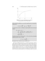
2 1. The Determinants of Market Outcomes
50
100
Q
P
Slope is −2
∆P
∆Q
Figure 1.1. (Inverse) demand function.

1.1.1.1 The Anatomy of a Demand Function
An individual’s demand function describes the amount of a good that a consumer
would buy as a function of variables that are thought to affect this decision such as
price P
i
and often income y. Figure 1.1 presents an example of an individual linear
demand function for a homogeneous product: Q
i
D 50  0:5P
i
or rather for the
inverse demand function, P
i
D 100  2Q
i
. More generally, we may write Q
i
D
D.P
i
;y/.
1
Inverting the demand curve to express price as a function of quantity
demanded and other variables yields the “inverse demand curve” P
i
D P.Q
i
;y/.
Standard graphs of an individual’s demand curve plot the quantity demanded of the
good at each level of its own price and take as a given the level of income and the

level of the prices of products that could be substitutes or complements. This means
that along a given plotted demand curve, those variables are fixed. The slope of the
demand curve therefore indicates at any particular point by how much a consumer
would reduce (increase) the quantity purchased if the price increased (decreased)
while income and any other demand drivers stayed fixed.
In the example in figure 1.1, an increase in price, P ,of€10 will decrease the
demand for the product by 5 units shown as Q. The consumer will not purchase
any units if the price is above 100 because at that point the price is higher than the
value that the customer assigns to the first unit of the good.
One interpretation of the inverse demand curve is that it shows the maximum price
that a consumer is willing to pay if she wants to buy Q
i
units of the good. While a
1
This will be familiar from introductory microeconomics texts as the “Marshallian” demand curve
(Marshall 1890).
1.1. Demand Functions and Demand Elasticities 3
consumer may value the first unit of the good highly, her valuation of, say, the one
hundredth unit will typically be lower and it is this diminishing marginal valuation
which ensures that demand curves typically slope downward. If our consumer buys
a unit only if her marginal valuation is greater than the price she must pay, then the
inverse demand curve describes our consumer’s marginal valuation curve.
Given this interpretation, the inverse demand curve describes the difference
between the customer’s valuation of each unit and the actual price paid for each
unit. We call the difference between what the consumer is willing to pay for each
unit and what he or she actually pays the consumer’s surplus available from that
unit. For concreteness, I might be willing to pay a maximum of €10 for an umbrella
if it’s raining, but may nonetheless only have to pay €5 for it, leaving me with a
measure of my benefit from buying the umbrella and avoiding getting wet, a surplus
of €5. At any price P

i
, we can add up the consumer surplus available on all of the
units consumed (those with marginal valuations above P
i
) and doing so provides
an estimate of the total consumer surplus if the price is P
i
.
In a market with homogeneous products, all products are identical and perfectly
substitutable. In theory this results in all products having the same price, which is
the only price that determines the demand. In a market with differentiated products,
products are not perfectly substitutable and prices will vary across products sold
in the market. In those markets, the demand for any given product is determined
by its price and the prices of potential substitutes. In practice, markets which look
homogeneous from a distance will in fact be differentiated to at least some degree
when examined closely. Homogeneity may nonetheless be a reasonable modeling
approximation in many such situations.
1.1.1.2 The Contribution of Consumer Theory: Deriving Demand
Demand functions are classically derived by using the behavioral assumption that
consumers make choices in a way that can be modeled as though they have an
objective, to maximize their utility, which they do subject to the constraint that they
cannot spend more than they earn.As is well-known to all students of microeconomic
theory, the existence of such a utility function describing underlying preferences
may in turn be established under some nontrivial conditions (see, for example, Mas-
Colell et al. 1995, chapter 1). Maximizing utility is equivalent to choosing the most
preferred bundle of goods that a consumer can buy given her wealth.
More specifically, economists have modeled a customer of type .y
i
;Â
i

/ as choos-
ing to maximize her utility subject to the budget constraint that her total expenditure
cannot be higher than her income:
V
i
.p
1
;p
2
;:::;p
J
;y
i
IÂ
i
/ D max
q
1
;q
2
;:::;q
J
u
i
.q
1
;q
2
;:::;q
J

IÂ
i
/
subject to p
1
q
1
C p
2
q
2
CCp
J
q
J
6 y
i
;
4 1. The Determinants of Market Outcomes
where p
j
and q
j
are prices and quantities of good j , u
i
.q
1
;q
2
;:::;q

J
IÂ
i
/ is the
utility of individual i associated with consuming this vector of quantities, y
i
is the
disposable income of individual i, and Â
i
describes the individual’s preference type.
In many empirical models using this framework, the “i” subscripts on the V and u
functions will be dropped so that all differences between consumers are captured
by their type .y
i
;Â
i
/.
Setting up this problem by using a Lagrangian provides the first-order conditions
@u
i
.q
1
;q
2
;:::;q
J
;y
i
IÂ
i

/
@q
j
D p
j
()
@u
i
.q
1
;q
2
;:::;q
J
;y
i
IÂ
i
/=@q
j
p
j
D  for j D 1;2;:::;J;
together with the budget constraint which must also be satisfied. We have a total of
J C1 equations in J C1 unknowns: the J quantities and the value of the Lagrange
multiplier, .
At the optimum, the first-order conditions describe that the Lagrange multiplier
is equal to the marginal utility of income. In some cases it will be appropriate to
assume a constant marginal utility of income. If so, we assume behavior is described
by a utility function with an additively separable good q

1
, the price of which is
normalized to 1, so that u
i
.q
1
;q
2
;:::;q
J
IÂ
i
/ DQu
i
.q
2
;:::;q
J
IÂ
i
/ Cq
1
and p
1
D
1. This numeraire good q
1
is normally termed “money” and its inclusion provides an
intuitive interpretation of the first-order conditions. In such circumstances a utility-
maximizing consumer will choose a basket of products so that the marginal utility

provided by the last euro spent on each product is the same and equal to the marginal
utility of money, i.e., 1.
2
More generally, the solution to the maximization problem describes the individ-
ual’s demand for each good as a function of the prices of all the goods being sold
and also the consumers’income. Indexing goods by j , we can write the individual’s
demands as
q
ij
D d
ij
.p
1
;p
2
;:::;p
J
Iy
i
IÂ
i
/; j D 1;2;:::;J:
A demand function for product j incorporates not only the effect of the own price
of j on the quantity demanded but also the effect of disposable income and the
price of other products whose supply can affect the quantity of good j purchased.
In figure 1.1, a change in the price of j represents a movement along the curve while
a change in income or in the price of other related goods will result in a shift or
rotation of the demand curve.
2
This is called a quasi-linear demand function and gives the result because the first-order condition

for good 1 collapses to
 D
@u
i
.q
1
;q
2
;:::;q
J
;y
i
I Â
i
/=@q
1
p
1
D
@u
i
.q
1
;q
2
;:::;q
J
;y
i
I Â

i
/
@q
1
;
which is the marginal utility of a monetary unit. That in turn is equal to one.
1.1. Demand Functions and Demand Elasticities 5
The utility generated by consumption is described by the (direct) utility function,
u
i
, which relates the level of utility to the goods purchased and is not observed. We
know that not all levels of consumption are possible because of the budget constraint
and that the consumer will choose the bundle of goods that maximizes her utility.
The indirect utility function V
i
.p; y
i
IÂ
i
/, where p D .p
1
;p
2
;:::;p
J
/, describes
the maximum utility a consumer can feasibly obtain at any level of the prices and
income. It turns out that the direct and indirect utility functions each can be used to
fully describe the other.
In particular, the following result will turn out to be important for writing down

demand systems that we estimate.
For every indirect utility function V
i
.p; y
i
IÂ
i
/ there is a direct utility function
u
i
.q
1
;q
2
;:::;q
J
IÂ
i
/ that represents the same preferences over goods provided
the indirect utility function satisfies some properties, namely that V
i
.p; y
i
IÂ
i
/ is
continuous in prices and income, nonincreasing in price, nondecreasing in income,
quasi-convex in .p; y
i
/ with any one element normalized to 1 and homogeneous

degree zero in .p; y
i
/.
This result sounds like a purely theoretical one, but it will actually turn out to be
very useful in practice. In particular, it will allow us to retrieve the demand function
q
i
.pIy
i
IÂ
i
/ without actually explicitly solving the utility-maximization problem.
3
Computationally, this is an important simplification.
1.1.1.3 Aggregation and Total Market Size
Individual consumers’ demand can be aggregated to form the market aggregate
demand by adding the individual quantities demanded by each customer at any
given price. If q
ij
D d
ij
.p
1
;p
2
;:::;p
J
Iy
i
IÂ

i
/ describes the demand for product
j by individual i, then aggregate (total) demand is simply the sum across individuals:
Q
j
D
I
X
iD1
q
ij
D
I
X
iD1
d
ij
.p
1
;p
2
;:::;p
J
;y
i
IÂ
i
/; j D 1;2;:::;J;
where I is the total number of people who might want to buy the good. Many
potential customers will set q

ij
D 0 at least for some sets of prices p
1
;p
2
;:::;p
J
even though they will have positive purchases at lower prices of some products. In
some cases, known as single “discrete choice” models, each individual will only buy
at most one unit of the good and so d
ij
.p
1
;p
2
;:::;p
J
;y
i
IÂ
i
/ will be an indicator
variable taking on the value either zero or one depending on whether individual i
buys the good or not at those prices. In such models, the total number of people
3
This result is known as a “duality” result and is often taught in university courses as a purely
theoretical equivalence result. For its very practical implications, see chapter 9, where we describe the
use of Roy’s identity to generate empirical demand systems from indirect utility functions rather than
the direct utility formulation.
6 1. The Determinants of Market Outcomes

who may want to buy the good is also the total potential market size. (We will
discuss discrete choice models in more detail in chapter 9.) On the other hand, when
individuals can buy more than one unit of the good, to establish the total potential
market size we need to evaluate both the total potential number of consumers and
also the total number of goods they might buy. Often the total potential number of
consumers will be very large—perhaps many millions—and so in many econometric
demand models we will approximate the summation with an integral.
In general, total demand for product j will depend on the full distribution of
income and consumer tastes in the population. However, under very special assump-
tions, we will be able to write the aggregate market demand as a function of aggregate
income and a limited set of taste parameters only:
Q
j
D D
j
.p
1
;p
2
;:::;p
J
;YIÂ/;
where Y D
P
I
iD1
y
i
.
For example, suppose for simplicity that Â

i
D  for all individuals and every
individual’s demand function is “additively separable” in the income variable so
that an individual’s demand function can be written
d
ij
.p
1
;p
2
;:::;p
J
;y
i
IÂ
i
/ D d

ij
.p
1
;p
2
;:::;p
J
I/ C ˛
j
y
i
;

where ˛
j
is a parameter common to all individuals, then aggregate demand for
product j will clearly only depend on aggregate income. Such a demand function
implies that, given the prices of goods, an increase in income will have an effect on
demand that is exactly the same no matter what the level of the prices of all of the
goods in the market. Vice versa, an increase in the prices will have the same effect
whatever the level of income.
4
The study of the conditions under which we can aggregate demand functions
and express them as a function of characteristics of the income distribution such as
the sum of individual incomes is called the study of aggregability.
5
Lessons from
that literature motivate the use of particular functional forms for demand systems in
empirical work such as the almost ideal demand system (AIDS
6
). In general, when
building empirical models we may well want to allow market demand to depend
on other statistics from the income distribution besides just the total income. For
example, we might think demand for a product depends on total income in the
population but also the variance, skewness, or kurtosis of the income distribution.
Intuitively, this is fairly clear since if a population were made up of 1,000 people
4
If consumer types are heterogeneous but are not observed by researchers, then an empirical aggre-
gate demand model will typically assume a parametric distribution for consumer types in a population,
f
Â
.ÂI /. In that case, the aggregate demand model will depend on parameters  of the distribution of
consumer types. We will explore such models in chapter 9.

5
For a technical discussion of the founding works, see the various papers by W. M. Gorman collected
in Gorman (1995). More recent work includes Lewbel (1989).
6
An unfortunate acronym, which has led some authors to describe the model as the nearly ideal
demand system (NIDS).
1.1. Demand Functions and Demand Elasticities 7
making €1bn and everyone else making €10,000, then sales of €15,000 cars would
be at most 1,000. On the other hand, the same total income divided more equally
could certainly generate sales of more than 1,000. (For recent work, see, for example,
Lewbel (2003) and references therein.)
1.1.2 Demand Elasticities
Elasticities in general, and demand elasticities in particular, turn out to be very
important for lots of areas of competition policy. The reason is that the “price elas-
ticity of demand” provides us with a unit-free measure of the consumer demand
response to a price increase.
7
The way in which demand changes when prices go
up will evidently be important for firms when setting prices to maximize profits
and that fact makes demand elasticities an essential part of, for example, merger
simulation models.
1.1.2.1 Definition
The most useful measurement of the consumer sensitivity to changes in prices is the
“own-price” elasticity of demand. As the name suggests, the own-price elasticity of
demand measures the sensitivity of demand to a change in the good’s own-price and
is defined as
Á
jj
D
%Q

j
%P
j
D
100.Q
j
=Q
j
/
100.P
j
=P
j
/
:
The demand elasticity expresses the percentage change in quantity that results from
a 1% change in prices. Alfred Marshall introduced elasticities to economics and
noted that one of their great properties is that they are unit free, unlike prices which
are measured in currency (e.g., euros per unit) and quantities (sales volumes) which
are measured in a unit of quantity per period, e.g., kilograms per year. In our example
in figure 1.1 the demand elasticity for a price increase of 10 leading to a quantity
decrease of 5 from the baseline position, where P D 60 and Q D 20,isÁ
jj
D
.5=20/=.10=60/ D1:5.
For very small variations in prices, the demand elasticity canbe expressed by using
the slope of the demand curve times the ratio of prices to quantities. A mathematical
result establishes that this can also be written as the derivative with respect to the
logarithm of price of the log transformation of demand curve:
Á

jj
D
P
j
Q
j
@Q
j
@P
j
D
@ ln Q
j
@ ln P
j
:
7
The term “elasticity” is sometimes used as shorthand for “price elasticity of demand,” which in turn
is shorthand for “the elasticity of demand with respect to prices.” We will sometimes resort to the same
shorthand terminology since the full form is unwieldy. That said, we do so with the caveat that, since
elasticities can be both “with respect to” and “of” anything, the terms elasticity or “demand elasticity” are
inherently ambiguous and therefore somewhat dangerous. We will, for example, talk about the elasticity
of costs with respect to output.
8 1. The Determinants of Market Outcomes
Demand at a particular price point is considered “elastic” when the elasticity is
bigger than 1 in absolute value.An elastic demand implies that the change in quantity
following a price increase will be larger in percentage terms so that revenues for a
seller will fall all else equal.An inelastic demand at a particular price level refers to an
elasticity of less than 1 in absolute value and means that a seller could raise revenues
by increasing the price provided again that everything else remained the same. The

elasticity will generally be dependent on the price level. For this reason, it does not
usually makes sense to talk about a given product having an “elastic demand” or
an “inelastic demand” but it should be said that it has an “elastic” or “inelastic”
demand at a particular price or volume level, e.g., at current prices. The elasticities
calculated for an aggregate demand are the market elasticities for a given product.
1.1.2.2 Substitutes and Complements
The cross-price elasticity of demand expresses the effect of a change in price of
some other good k on the demand for good j . A new, higher, price for p
k
may,
for instance, induce some consumers to change their purchases of product j .If
consumers increase their purchases of product j when p
k
goes up, we will call
products j and k demand substitutes or just substitutes for short.
Two DVD players of different brands are substitutes if the demand for one of
them falls as the price of the other decreases because people switch across to the
now relatively cheaper DVD player. Similarly, a decrease in prices of air travel may
reduce the demand for train trips, holding the price of train trips constant.
On the other hand, the new higher price of k may induce consumers to buy less of
good j . For example, if the price of ski passes increases, perhaps fewer folk want to
go skiing and so the demand for skiing gear goes down. Similarly, if the price of cars
increases, the demand for gasoline may well fall. When this happens we will call
products j and k demand complements or just complements for short. In this case,
the customer’s valuation of good j increases when good k has been purchased:
8
Á
jk
D
8

ˆ
ˆ
<
ˆ
ˆ
:
P
k
Q
j
@Q
j
@P
k
>0 and
@Q
j
@P
k
>0 if products are substitutes;
P
k
Q
j
@Q
j
@P
k
<0 and
@Q

j
@P
k
<0 if products are complements:
8
Generally, this terminology is satisfactory for individual demand functions but can become unsat-
isfactory for aggregate demand functions, where it may or may not be the case that @Q
j
=@P
k
D
@Q
k
=@P
j
since in that case the complementary (or substitute) links between the products may be of
differing strengths. See, in particular, the discussion in the U.K. Competition Commission’s investi-
gation into Payment Protection Insurance (PPI) at, for example, www.competition-commission.org.uk/
inquiries/ref2007/ppi/index.htm. In that case, some evidence showed that loans and insurance covering
unemployment, accident, and sickness were complementary only in the sense that the demand for insur-
ance was affected by the credit price while the demand for credit appeared largely unaffected by the price
of the accompanying PPI. That investigation (chaired by one of the authors) found it useful to introduce a
distinction between one-sided and two-sided complementarity. An analogous distinction could be made
for asymmetric demand substitution patterns.
1.1. Demand Functions and Demand Elasticities 9
1.1.2.3 Short Term versus Long Term
Most demand functions are static demand functions—they consider how consumers
allocate their demand across products at a given point in time. In general, particularly
in markets for durable goods, or goods which are storable, we will expect to have
important intertemporal linkages in demand. The demand for cars today may depend

on tomorrow’s price as well as today’s price. If so, demand elasticities in the long run
may well be different from the demand elasticities in the short run. In some cases the
price elasticity of demand will be higher in the short run. This happens for instance
when there is a temporary decrease in prices such as a sale, when consumers will
want to take advantage of the temporarily better prices to stock up, increasing the
demand in the short run but decreasing it at a later stage (see, for example, Hendel
and Nevo 2006a,b). In this case, the elasticity measured over a short period of time
would overestimate the actual elasticity in the long run. The opposite can also occur,
so that the long-run elasticity at a given price is higher than the short-run elasticity.
For instance, the demand for petrol is fairly inelastic in the short run, since people
have already invested in their cars and need to get to work. On the other hand, in
the long run people can adjust to higher petrol prices by downsizing their car.
1.1.3 Introduction to Common Demand Specifications
We often want to estimate the effect of price on quantity demanded. To do so we
will typically write down a model of demand whose parameters can be estimated.
We can then use the estimated model to quantify the impact of a change in price
on the quantity being demanded. With enough data and a general enough model
our results will not be sensitive to this choice. However, with realistic sample sizes,
we often have to estimate models that impose a considerable amount of structure
on our data sets and so the results can be sensitive to the demand specification
chosen. That unfortunate reality means one should choose demand specifications
with particular care. In particular, we need to be clear about the properties of the
estimated model that are being determined by the data and the properties that are
simply assumed whatever the estimated parameter values. An important aspect of
the demand function will be its curvature and how this changes as we move along the
curve. The curvature of the demand curve will determine the elasticity and therefore
the impact of a change in price on quantity demanded.
1.1.3.1 Linear Demand
The linear demand is the simplest demand specification. The linear demand function
can be written Q

i
D a  bP with analogous inverse demand curve
P D
a
b

1
b
Q
i
:
In each case, a and b are parameters of the model (see figure 1.2).
10 1. The Determinants of Market Outcomes
Q
P
a
a
/ b
Slope is −1 / b
Figure 1.2. The linear demand function.
The slope of the inverse demand curve is
@P
@Q
D
1
b
:
The intercepts are a=b at Q D 0 and a at P D 0. The linear demand implies that the
marginal valuation of the good keeps decreasing at a constant rate so that, even if
the price is 0 the consumer will not “buy” more than a units. Since most analysis in

competition cases happens at positive prices and quantities of the goods, estimation
results will not generally be sensitive to assumptions made about the shape of the
demand curve at the extreme ends of the demand function.
9
The elasticity for the
linear demand function is
Á D .b/
P
Q
:
Note that, unlike the slope, the elasticity of demand varies along the linear demand
curve. Elasticities generally increase in magnitude as we move to lower quantity
levels because the variations in quantity resulting from a price increase are larger
as a percentage of initial sales volumes. Because of its lack of curvature, the linear
demand will sometimes produce higher elasticities compared with other demand
specifications and therefore sometimes predicts lower price increases in response
to mergers and higher quantity adjustments in response to increases in price. As an
extreme example, consider an alternative inverse demand function which asymptotes
as we move leftward in the graph toward the price axis where Q D 0. In that case,
only very large price increases will drive significant quantity changes at low levels of
9
We rarely get data from a market where goods have been sold at zero prices. As we discuss below,
calculations such as consumer surplus on the other hand may sometimes be very sensitive to such
assumptions.
1.1. Demand Functions and Demand Elasticities 11
P
Q
Q = 0 means elasticity is −∞
P
/ Q = −1 / b means elasticity is −1

P = 0 means elasticity is 0
Figure 1.3. Demand elasticity values in the linear demand curve.
output or, analogously, small price changes will drive only small quantity changes,
i.e., a low elasticity of demand. An example in the form of the log-linear demand
curve is provided below. In contrast, the linear demand curve generates an arbitrarily
large elasticity of demand (large in magnitude) as we move toward the price axis on
the graph (see figure 1.3).
1.1.3.2 Log-Linear Demand
The one exception to the rule that elasticities depend on the price level is the log-
linear demand function, which has the form
Q D D.P / D e
a
P
b
:
Taking natural logarithms turns the expression into a demand equation that is linear
in its parameters:
ln Q D a  b ln P:
This specification is particularly useful because many of the estimation techniques
used in practice are most easily applied to models which are linear in their param-
eters. Expressing effects in terms of percentages also provides us with results that
are easily interpreted. The inverse demand which corresponds to figure 1.4 can be
written
P D P.Q/ D .e
a
Q/
1=b
:
When prices increase toward infinity, if b>0then the quantity demanded tends
toward 0 but never reaches it. An assumption embodied in the log-linear model is

that there will always be some demand for the good, no matter how expensive it is.
Similarly, the demand tends to infinity when the price of the good approaches 0.
12 1. The Determinants of Market Outcomes
Q
P
Figure 1.4. The log-linear demand curve.
As a product approaches the zero price, consumers are willing to have an unlimited
amount of it:
lim
P !1
D.P / D e
a
lim
P !1
P
b
D 0;
lim
Q!1
P.Q/ D lim
Q!1
.e
a
Q/
1=b
D 0:
The log-linear demand also has a constant elasticity over the entire demand curve,
which is a unique characteristic of this functional form:
Á D
@ ln Q

@ ln P
Db:
As a result the log-linear demand model is sometimes referred to as the constant
elasticity or iso-elastic demand model. Price changes do not affect the demand
elasticity, which means that if we have one estimate of the elasticity, at a given
price, this estimate will—rather conveniently but perhaps optimistically—be the
same for all price points. Of course, if in truth the price sensitivity of demand does
depend on the price level, then this iso-elasticity assumption will be a strong one
imposed by the model whatever values we estimate its parameters a and b to take
on. Empirically, given enough data, we can tell apart data generated by the linear
demand model and the log-linear model since movements in supply at different
price levels will provide us with information about the slope of demand and hence
elasticities. Formally, we can use a “Box–Cox” test to distinguish the models (see,
for example, Box and Cox 1964).
1.1.3.3 Discrete Choice Demand Models
Consumer choice situations can be sometimes best represented as zero–one “dis-
crete” decisions between different alternative options. Consider, for example, buy-
ing a car. The choice is “which car” rather than “how-much car.” In such situations,